On shifted cardinal interpolation by Gaussians and multiquadricsB. J. C. BaxterDepartment of MathematicsImperial College of Science, Technology and Medicine180 Queen's Gate, London SW7 2BZ, EnglandE-mail: b.baxter@ic.ac.ukWWW: http://www.ma.ic.ac.uk/�baxter/baxter.htmlN. SivakumarCenter for Approximation TheoryDepartment of MathematicsTexas A & M UniversityCollege Station, TX 77843-3368, USAE-mail: sivan@math.tamu.eduWWW: http://www.math.tamu.edu/�sivanAbstractA radial basis function approximation is a linear combination of translates of a �xed function':Rd ! R. Such functions possess many useful and interesting properties when the translatesare integers and ' is radially symmetric. We study the closely related problem for which the �xedfunction is the shifted Gaussian ' = G(���), where G(x) = exp(��kxk22) and � 2 Rd. Speci�cally,we exploit the theory of elliptic functions to establish the invertibility of the Toeplitz operator('(�+ j � k))j;k2Zdwhen � has no half-integer components; it is singular otherwise. This implies the existence of ashifted Gaussian cardinal function, that is, a linear combination � of integer translates of the shiftedGaussian satisfying �(j) = �0j . We also study shifted cardinal functions when the parameter � tendsto zero. In particular, we discover their uniform convergence to the sinc function when the shiftvector � possesses no half-integer components. Our methods are based in part on similar resultsestablished by the �rst author when the basis function is the Hardy multiquadric. Several intriguinglinks with the theory of shifted B-spline cardinal interpolation are described in the �nale.1

baxter and sivakumar1. IntroductionA radial basis function approximant is a linear combination of translates of a �xed function, or somesuitable limit of such approximants. Thus we considers(x) = Xk2Zd ak'(x� bk); x 2 Rd; (1:1)where (bk)k2Zd is some �xed set of distinct points, or centres, in Rd, and (ak)k2Zd is a sequence ofreal numbers satisfying conditions ensuring (1.1) is meaningful; for example, we might require thescalar sequence to be �nitely supported, or for the in�nite series in (1.1) to be absolutely convergentat every point x 2 Rd. Such functions provide a exible and useful approach to multivariate inter-polation (see, for example, the survey articles [P, Bu3]). Much of the existing literature concentrateson the special case when the centres form an in�nite grid and ' is radially symmetric; we refer thereader to the fundamental papers [Bu1, Bu2] of Buhmann on cardinal interpolation. Here we studythe closely related problem of shifted Gaussian cardinal interpolation, which means that our typicalapproximant is s(x) = Xk2Zd ak'(x+ �� k); x 2 Rd; (1:2)where the shift � is a �xed vector in Rd and the function '(x) = exp(��kxk22) is a Gaussian. Weshall also allow the (positive) parameter � to vary. First, let us recall that the cardinal function ��for the shifted Gaussian must satisfy��(j) = �0j ; j 2 Zd; (1:3)where ��(x) = Xk2Zd ck(�)'(x+ �� k); x 2 Rd: (1:4)Our main �nding is that such cardinal functions exist when the shift vector � has no half-integercomponents, the term half-integer connoting an element of 12 + Z in this paper, and we shall callsuch shifts admissible. The technique is founded on analysis of the non-Hermitian Toeplitz operator�'(�+ j � k)�j;k2Zdusing its close links with the theory of Jacobian Theta functions developed by the �rst author in [B1].This analysis is to be found in Section 2. In Section 3, we prove that admissibly shifted cardinalfunctions converge uniformly to the sinc function as the parameter � tends to zero. Moreover, we2

shifted cardinal interpolationalso show that the admissibly shifted cardinal interpolants to a square-integrable function convergeto this function in the mean-square sense if and only if it is band limited. These studies indicate thatexcellent accuracy can be attained when approximating band-limited functions by shifted Gaussiansif the parameter � is suitably small. We suspect that this is mostly responsible for the favourableresults found in, say, the applications of Gaussian radial basis functions in neural net problems (see,for instance [BL]).The methods employed in Section 3 are based in part on similar results established by the �rstauthor in [B2] when the basis function is the Hardy multiquadric '(x) = (kxk22 + c2)1=2 and theparameter c tends to in�nity; we discuss this connection in Section 4. Furthermore, our Gaussianresearches shed some light on shifted multiquadric interpolation, and these implications are alsooutlined in Section 4. Finally, Section 5 describes the intriguing parallels between the theory ofshifted B-spline cardinal interpolation and this paper.2. Shifted Gaussians, Toeplitz forms and Theta functionsLet � be a positive constant, let ':R! R be the Gaussian '(x) = exp(��x2), x 2 R, and de�nethe shifted Gaussian '�(x) = '(x + �), where � is a real number. We consider the bi-in�niteToeplitz matrix A(�) := �'�(j � k)�j;k2Z ; � 2 R; (2:1)as a linear operator on `2(Z). The classical theory of Toeplitz forms (see [W] or [GS]) studies A(�)via the symbol functionG�(�) � G�(�; �) := Xk2Z '�(k) exp(�ik�); � 2 R; (2:2)and we recall the well-known fact that A(�) : `2(Z)! `2(Z) is invertible if and only if the symbolfunction does not vanish [W, Theorem 1]. Following [B1], we �nd that G� is a multiple of the Thetafunction #(z) � #(z; q) := Xk2Z qk2zk ; z 2 C n f0g; for q 2 C and jqj < 1: (2:3)Speci�cally, some elementary algebraic manipulation reveals the identityG�(�; �) = q�2#(q2�e�i�) where q = e��: (2:4)Thus the invertibility of A(�) is determined by the zero structure of the associated Theta function.Therefore we present below some salient properties of Theta functions needed later in the paper.3

baxter and sivakumarLemma 2.1. The Theta function enjoys the in�nite product formula#(z) = T (q) 1Yk=0(1+q2k+1z)(1+q2k+1z�1); z 2 C nf0g; where T (q) := 1Y=1(1�q2`): (2:5)Proof. See [WW, Section 21.3], [Be, Section 32].Corollary 2.2. The zeros of # are given by f�q` : ` 2 Z odd g.Proof. Equation (2.5) implies that #(z) = 0 if and only if 1 + q2k+1z�1 = 0 for some non-negativeinteger k.Proposition 2.3. The function f� 7! j#(q2�e�i�)j2 : � 2 Rg is even, 2�-periodic, and decreasesfor 0 � � � �.Proof. The function is evidently even and 2�-periodic. Furthermore, (2.5) yields the in�nite productj#(q2�e�i�)j2 = T (q)2 1Yk=0(1 + q2k+1+2�e�i�)(1 + q2k+1+2�ei�)(1 + q2k+1�2�ei�)(1 + q2k+1�2�e�i�)= T (q)2 1Yk=0(1 + 2q2k+1+2� cos � + q4k+2+4�)(1 + 2q2k+1�2� cos � + q4k+2�4�); (2:6)and we see that each of the terms in the �nal product is decreasing for 0 � � � �.Proposition 2.4. <#(q2�w) � 0 when jwj = 1 and � 2 [�1=2; 1=2], with equality if and only ifw = �1 and � = �1=2.Proof. It su�ces to prove this for 0 � � � 1=2 because of the equation #(q�2�w) = #(q2�w). Nowthe Theta function is a conformal mapping from the open annulus fz 2 C : q < jzj < 1g onto thedomain whose boundaries are the images under # of the boundaries of the annulus. It is shown in[B1, Lemma 2.7] that # maps the unit circle fz 2 C : jzj = 1g onto the real interval [#(�1); #(1)].Thus it su�ces to prove that <#(qw) � 0 when jwj = 1. But (2.5) supplies the expression#(qw) = T (q) 1Yk=0(1 + q2k+2w)(1 + q2kw) = (1 + w)T (q)��� 1Yk=0(1 + q2kw)���2;whence <#(qw) = (1 + <w)T (q)jQ1k=0(1 + q2kw)j2 � 0 with equality if and only if w = �1.All the results obtained hitherto will be used in the sequel. We commence with an invertibilitytheorem for A(�).Theorem 2.5. The symbol function G�, de�ned by (2.2), has no zeros unless � is a half-integer.Equivalently, the bi-in�nite Toeplitz matrix A(�) of (2.1) is invertible on `2(Z) if and only if � isnot a half-integer. 4

shifted cardinal interpolationProof. Corollary 2.2 and (2.4) imply that the symbol function G�(�; �) = 0 if and only if 2� is anodd integer and e�i� = �1. The equivalence follows from [W, Theorem 1].This result was found independently by R. A. Rahim [R], whose technique was quite di�erent.Given the invertibility of A(�) when � =2 1=2+Z , it is natural to consider the condition numbercond2A(�) := kA(�)k kA(�)�1k for such � (the norm used here is the operator norm on `2(Z)).Theorem 2.6. Let � = �0 + `, where j�0j < 1=2 and ` is an integer. Thencond2A(�) = #(q2�0)#(�q2�0) : (2:7)Proof. The spectrum of the bi-in�nite Hermitian Toeplitz matrix A(�)�A(�) is given by the rangeof its symbol function fjG�(�)j2 : �� � � � �g (see [W, Theorem 1']). Therefore kA(�)�A(�)k= maxfjG�(�)j2 : �� � � � �g, by [Bo, p. 175, Theorem 11(c)]. Furthermore, kA(�)k2 =kA(�)�A(�)k by [Bo, p. 157, Theorem 2], which yields kA(�)k = maxfjG�(�)j : �� � � � �g.Similarly kA(�)�1k = maxfjG�(�)j�1 : �� � � � �g. Thuscond2A(�) = maxfjG�(�)j : � 2 [��; �]gminfjG�(�)j : � 2 [��; �]g= maxfjG�0(�)j : � 2 [��; �]gminfjG�0(�)j : � 2 [��; �]g= maxfj#(q2�0w)j : w 2 C; jwj = 1gminfj#(q2�0w)j : w 2 C; jwj = 1g= ��� #(q2�0)#(�q2�0) ���; (2:8)by (2.2), (2.4) and Proposition 2.3. Finally, Proposition 2.4 entails the non-negativity of #(�q2�0).Equation (2.7) re ects the fact that cond2A(�) is a 1-periodic function of the shift parameter�. Our next result shows that the condition number increases as j�j grows from zero to half.Theorem 2.7. The function f� 7! cond2A(�) : �1=2 < � < 1=2g is even, increasing on [0; 1=2),and tends to in�nity as � tends to 1=2.Proof. Theorem 2.6 and Lemma 2.1 provide the relationscond2A(�) = #(q2�)#(�q2�) = 1Yk=0 1 + q2k+1(q2� + q�2�) + q4k+21� q2k+1(q2� + q�2�) + q4k+2= 1Yk=0 1 + 2q2k+1 cosh(2��) + q4k+21� 2q2k+1 cosh(2��) + q4k+2 ; (2:9)5

baxter and sivakumarand this last expression is clearly an even function of �. Further, each term in the numerator of theproduct increases for 0 � � � 1=2, whereas each term in the denominator decreases for 0 � � � 1=2.Finally, as � tends to 1=2, the �rst term (k = 0) in the denominator tends to zero.It is interesting, but seemingly irrelevant, that the in�nite product obtained in (2.9) is a multipleof the Jacobian elliptic function dn.We now take up the analysis of the semi-in�nite Toeplitz matrixA+(�) := ('�(j � k))j;k�0; � 2 R; (2:10)viewed as a linear operator on `2(Z+); here '�(x) = e��(x+�)2 and `2(Z+) denotes the sequencespace f(ak)k�0 : P1k=0 jakj2 < 1g. The interaction between the symbol function and the semi-in�nite Toeplitz operator is more subtle than in the bi-in�nite case. We recall that a semi-in�niteToeplitz matrix associated with a continuous symbol � is invertible on `2(Z+) if and only if � isnowhere zero and the curve f�(t) : �� � t � �g does not wind about zero [W, Theorem 5].Proposition 2.8. Suppose � is not a half-integer. Then fG�(�) : �� � � � �g does not windabout zero if and only if j�j < 1=2.Proof. If j�j < 1=2, then Proposition 2.4 yields <#(q2�e�i�) > 0 for all � 2 [��; �]. Hence<G�(�) = q�2<#(q2�e�i�) is positive for all � 2 [��; �]; a fortiori fG�(�) : �� � � � �g does notwind about zero.Conversely, let � = �0+`, where j�0j < 1=2 and ` 2 Znf0g. Since G�(�) = ei`�G�0(�) by (2.2)and fG�0(�) : �� � � � �g does not wind about the origin, we conclude that fG�(�) : �� � � � �gwinds about zero exactly ` times.Theorem 2.9. Suppose � 2 R. The following are equivalent:(i) j�j < 1=2;(ii) G� is nowhere zero and the winding number of the curve fG�(�) : �� � � � �g about zero iszero.(iii) The semi-in�nite Toeplitz matrix A+(�) de�ned in (2.10) is invertible on `2(Z+).Proof. (i) , (ii) This follows from Theorem 2.5 and Proposition 2.8.(ii) , (iii) This is [W, Theorem 5].We close this section with multivariate extensions of Theorems 2.5 and 2.6. Let '(d)(x) :=exp(��kxk22), x 2 Rd, � > 0, and let '(d)� (x) := '(d)(x + �), � 2 Rd. Consider the multivariate6

shifted cardinal interpolationToeplitz matrix (see [BM]) A(d)(�) := ('(d)� (j � k))j;k2Zd; � 2 Rd; (2:11)as a linear operator on `2(Zd). The symbol function G(d)� of A(d)(�) is given byG(d)� (�) � G(d)� (�; �) := Xk2Zd '(d)� (k) exp(�ikT �); � 2 Rd: (2:12)Clearly G(d)� is a tensor product of univariate symbol functions, to witG(d)� (�) = dYk=1G�k(�k); � = (�1; : : : ; �d); � = (�1; : : : ; �d):Consequently, Theorems 2.5 and 2.6 have multivariate analogues.Theorem 2.10. The multivariate Toeplitz matrix A(d)� de�ned in (2.11) is invertible on `2(Zd) ifand only if no co-ordinate of the vector shift � = (�1; : : : ; �d) is a half-integer.Proof. In view of (2.4) and Corollary 2.2, G(d)� (�) = 0, � = (�1; : : : ; �d), if and only if 2�k is an oddinteger and �k is an odd integral multiple of � for some k 2 f1; : : : ; dg.Theorem 2.11. Suppose � = �0 + `, where �0 2 (�1=2; 1=2)d and ` 2 Zd. Thencond2A(d)(�) = dYk=1 #(q2�0k)#(�q2�0k) ; �0 = (�01; : : : ; �0d); q = e��:Proof. The symbol function for A(d)(�)�A(d)(�) is fjG(d)� (�)j2 : � 2 [��; �]dg = fQdk=1 jG�k(�k)j2 :� = (�1; : : : ; �d) 2 [��; �]dg. The remainder of the proof is a simple consequence of (2.8).3. Shifted Gaussian cardinal interpolation and entire functions of exponential typeLet � be positive and de�ne the Gaussian '�(x) = exp(��x2), x 2 R, and its shift '�;� = '�(�+�),� 2 R; we have changed notation slightly to emphasize dependence on the parameter �. We haveseen that the symbol function G�(�; �) does not vanish when � is not a half-integer, in which casewe can de�ne the cardinal function ��;� associated with '�;� by its Fourier transform:d��;�(�) := b'�;�(�)G�(�; �); � 2 R; (3:1)where b'�;�(�) = ('�(�+ �)) (�). It is well known that��;�(x) = Xk2Z ck(�; �)'�;�(x� k); x 2 R; (3:2)7

baxter and sivakumarwhere ck(�; �) = (2�)�1 Z ��� G�(�; �)�1 exp(�ik�) d�; k 2 Z ; (3:3)and ��;�(j) = �0j ; j 2 Z : (3:4)The multivariate cardinal function �(d)�;� is de�ned similarly by its Fourier transformb�(d)�;�(�) := b'(d)�;�(�)G(d)� (�; �); � 2 Rd; (3:5)provided the shift vector � is admissible, that is, none of its components is a half-integer. (Hereand elsewhere, '(d)�;�(x) = '(d)� (x + �), where '(d)� (x) := exp(��kxk22), x; � 2 Rd; also b'(d)�;�(�) =('(d)(�+ �)) (�), and b�(d)�;�(�) = (�(d)�;�(�)) (�).) In this section we shall study some properties of thelinear space span f�(d)�;�(� � k) : k 2 Zdgas the parameter � approaches zero.The function b�(d)�;� de�ned in (3.5) inherits the tensor-product structure from the Gaussian andthe corresponding symbol. Precisely, we have the useful relationb�(d)�;�(�) = dYk=1 b'�;�k(�k)G�k(�k; �) ; � = (�1; : : : ; �d); � = (�1; : : : ; �d): (3:6)Primarily because of this tensor-product relation, all of the multivariate results considered in thissection can be derived from their univariate counterparts. Therefore we address the univariatetopics �rst.Poisson summation provides a useful alternative formula for the Fourier transform of the Gaus-sian cardinal function: d��;�(�) = �1 +E�;�(�)��1; (3:7)where E�;�(�) = Xk2Znf0g b'�;�(� + 2�k)b'�;�(�) ; � 2 R: (3:8)We shall often infer the behaviour of d��;� from that of E�;�. It will also be convenient to de�neE� � E�;0. 8

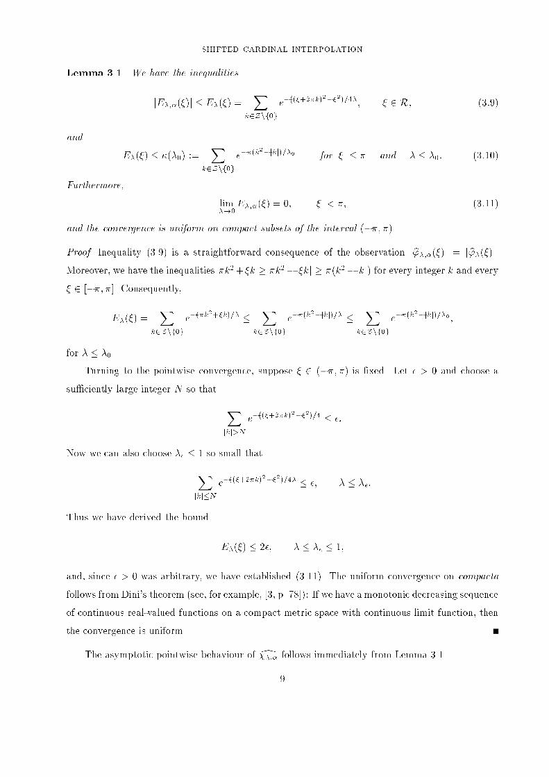
shifted cardinal interpolationLemma 3.1. We have the inequalitiesjE�;�(�)j � E�(�) = Xk2Znf0ge�((�+2�k)2��2)=4�; � 2 R; (3:9)and E�(�) � �(�0) := Xk2Znf0ge��(k2�jkj)=�0 for j�j � � and � � �0: (3:10)Furthermore, lim�!0E�;�(�) = 0; j�j < �; (3:11)and the convergence is uniform on compact subsets of the interval (��; �).Proof. Inequality (3.9) is a straightforward consequence of the observation jb'�;�(�)j = jb'�(�)j.Moreover, we have the inequalities �k2+�k � �k2�j�kj � �(k2�jkj) for every integer k and every� 2 [��; �]. Consequently,E�(�) = Xk2Znf0ge�(�k2+�k)=� � Xk2Znf0ge��(k2�jkj)=� � Xk2Znf0ge��(k2�jkj)=�0 ;for � � �0.Turning to the pointwise convergence, suppose � 2 (��; �) is �xed. Let � > 0 and choose asu�ciently large integer N so that Xjkj>N e�((�+2�k)2��2)=4 � �:Now we can also choose �� � 1 so small thatXjkj�N e�((�+2�k)2��2)=4� � �; � � ��:Thus we have derived the bound E�(�) � 2�; � � �� � 1;and, since � > 0 was arbitrary, we have established (3.11). The uniform convergence on compactafollows from Dini's theorem (see, for example, [3, p. 78]): If we have a monotonic decreasing sequenceof continuous real-valued functions on a compact metric space with continuous limit function, thenthe convergence is uniform.The asymptotic pointwise behaviour of d��;� follows immediately from Lemma 3.1.9

baxter and sivakumarTheorem 3.2. If � is not a half-integer and � 2 (��; �), thenlim�!0 d��;�(� + 2�j) = �0j ; j 2 Z ; (3:12)and the convergence is uniform on compact subsets of (��; �).Proof. Equations (3.7) and (3.11) imply (3.12) when j = 0. When j 6= 0, we havejd��;�(� + 2�j)j= jd��;�(�)j��� b'�;�(� + 2�j)b'�;�(�) ��� = jd��;�(�)je�((�+2�j)2��2)=4�;which tends to zero as � ! 0 because d��;�(�) ! 1 and (� + 2�j)2 � �2 > 0 for j�j < � andj 6= 0. Uniform convergence on compact subsets of (��; �) follows from that of E�;�(�) ande�((�+2�j)2��2)=4�.Knowledge of the pointwise behaviour almost everywhere is not su�cient for the integral limitsstudied below. However, Lemma 3.3, and its consequence Corollary 3.4, will allow us to use thedominated convergence theorem later. Once more the panoply of Theta function theory comes toour aid, in particular the in�nite product (2.5).Lemma 3.3. Let q � q0 < 1 and let z = reit, where r 2 [q; q�1] and jtj < �. Then we obtain theinequalities (i) j#(z; q)j � T (q0); jtj � �=2; (3:13)and (ii) j#(z; q)j � T (q0)3 sin2 t; �=2 < jtj < �; (3:14)using the notation of Lemma 2.1.Proof.(i)When jtj � �=2, we have < �1 + q2k+1r�1 exp(�it)� � 1. Hence every term in the in�nite product(2.5) has modulus exceeding one, which implies j#(q; z)j � T (q). Furthermore, T (q) � T (q0) forq � q0, yielding (3.13).(ii) For k � 1 and for any t 2 R, the triangle inequality providesj1 + q2k+1r�1e�itj � 1� q2k � 1� q2k0 ;because q � r � q�1. Hencej#(z; q)j � T (q0)3j(1 + qreit)(1 + qr�1e�it)j:10

shifted cardinal interpolationNow j1 + qr�1 exp(�it)j � inffj1 + � exp(�it)j : � � 0g = j sin tj, the last equation resulting fromelementary geometry; this proves (3.14).The preceding result can be used to derive a upper bound on the Fourier transform of theshifted Gaussian cardinal function. Speci�cally, if the shift � is not a half-integer, then the Fouriertransform of the Gaussian cardinal function takes the formd��;�(�) = b'�;�(�)Pk2Z b'�;�(� + 2�k) = �Xk2Z e2�ki�e�(��=�)ke��2k2=���1 = #(z; q)�1; (3:15)where q = exp(��2=�) and z = q�=� exp(2�i�). Therefore the lower bounds of (3.13) and (3.14)supply upper bounds for the modulus of d��;�.Corollary 3.4. Suppose � is not a half-integer; let 0 < � � �0 and set q0 = exp(��2=�0),q = exp(��2=�). There is a constant C(�; �0) for whichjd��;�(�)j � C(�; �0); � � �0; j�j � �: (3:16)Proof. It su�ces to restrict attention to � 2 (�1=2; 1=2) because the function f� 7! jd��;�j : � 2 Rgis 1-periodic; for j�j < 1=2, however, (3.16) follows from (3.13) and (3.14) via (3.15).Of course, C(�; �0)!1 as �! �1=2.Armed with these results, let us introduce the family of linear spacesV�;� := (Xk2Z ak��;�(� � k) : (ak)k2Z 2 `2(Z)) ; � > 0: (3:17)The exponential decay of ��;� for large argument implies the pointwise convergence of the seriesfor every square-summable sequence. In fact, as will have been immediate to readers familiar withthe theory of wavelets, very V�;� is a subspace of L2(R). More precisely, the integer translatesf��;�(� � k) : k 2 Zg form a Riesz basis for L2(R), as we now demonstrate.Proposition 3.5. Suppose � is not a half-integer and 0 < � � �0. There exist constants K1(�; �0)and K2(�; �0) for whichK1(�; �0)Xk2Z jakj2 � Xk2Z ak��;�(� � k) 2L2(R) � K2(�; �0)Xk2Z jakj2; (ak)k2Z 2 `2(Z): (3:18)Proof. It su�ces to prove (3.18) when the sequence (ak)k2Z is �nitely supported, because suchsequences form a dense subset of `2(Z). Setting A(�) := Pk2Z ak exp(�ik�) and applying the11

baxter and sivakumarParseval-Plancherel theorem, we obtain Xk2Z ak��;�(� � k) 2L2(R) = (2�)�1 ZR jA(�)j2jd��;�(�)j2 d�= (2�)�1 Z ��� jA(�)j2Xk2Z jd��;�(� + 2�k)j2 d�:NowXk2Z jd��;�(�+2�k)j2 = jd��;�(�)j2�1+ Xk2Znf0g ���� b'�;�(� + 2�k)b'�;�(�) ����2� = jd��;�(�)j2�1+E�=2(�)�: (3:19)Thus (3.10), (3.16) and Parseval's theorem imply Xk2Z ak��;�(� � k) 2L2(R) � C(�; �0)2�1 + �(�0=2)�Xk2Z jakj2;for � � �0. Finally, (3.7), (3.9) and (3.10) provide the inequalityjd��;�(�)j2 � (1 + �(�0))�2; j�j � �; � � �0;whence the estimate Xk2Z ak��;�(� � k) 2L2(R) � (1 + �(�0))�2 Xk2Z jakj2; � � �0;obtains from (3.19) and Parseval's theorem.The foregoing result implies that the family of linear maps fT�;�: `2(Z)! L2(R) : 0 < � � �0g,where T�;� : (ak)k2Z 7!Xk2Z ak��;�(� � k);is uniformly bounded. It follows that the image of V�;� under the Fourier transform F is given bythe succinct expression dV�;� = d��;�L2[��; �]; (3:20)being the composition F � T�;�(V�;�). That is, every member of dV�;� is an element of L2[��; �]multiplied by d��;�. (Here we are using the Riesz-Fischer theorem to pair `2(Z) and L2[��; �] viathe Fourier coe�cient sequence.)Now (3.12) implies the limiting relationlim�!0 dV�;� = f bf 2 L2(R) : bf is supported by [��; �] g =: cE� : (3:21)We have chosen the notationcE� because its inverse Fourier transform E� is precisely the set of entirefunctions of exponential type �; this is the celebrated Paley-Wiener theorem (see, for instance, [SW,pages 108�]). Thus it is natural to ask whether V�;� ! E� in some sense, and the answer to thisquestion is particularly elegant in L2(R). We shall need a speci�c form of the Poisson summationformula. 12

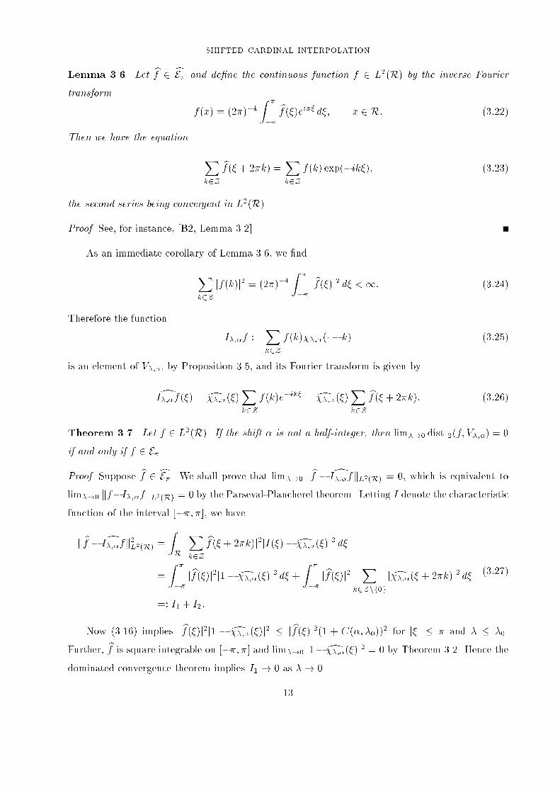
shifted cardinal interpolationLemma 3.6. Let bf 2 cE� and de�ne the continuous function f 2 L2(R) by the inverse Fouriertransform f(x) = (2�)�1 Z ��� bf (�)eix� d�; x 2 R: (3:22)Then we have the equation Xk2Z bf(� + 2�k) = Xk2Z f(k) exp(�ik�); (3:23)the second series being convergent in L2(R).Proof. See, for instance, [B2, Lemma 3.2].As an immediate corollary of Lemma 3.6, we �ndXk2Z jf(k)j2 = (2�)�1 Z ��� j bf(�)j2 d� <1: (3:24)Therefore the function I�;�f := Xk2Z f(k)��;�(� � k) (3:25)is an element of V�;�, by Proposition 3.5, and its Fourier transform is given bydI�;�f(�) = d��;�(�)Xk2Z f(k)e�ik� = d��;�(�)Xk2Z bf (� + 2�k): (3:26)Theorem 3.7. Let f 2 L2(R). If the shift � is not a half-integer, then lim�!0 dist 2(f; V�;�) = 0if and only if f 2 E�.Proof. Suppose bf 2 cE�. We shall prove that lim�!0 k bf � dI�;�fkL2(R) = 0, which is equivalent tolim�!0 kf�I�;�fkL2(R) = 0 by the Parseval-Plancherel theorem. Letting I denote the characteristicfunction of the interval [��; �], we havek bf � dI�;�fk2L2(R) = ZR jXk2Z bf(� + 2�k)j2jI(�)� d��;�(�)j2 d�= Z ��� j bf(�)j2j1� d��;�(�)j2 d� + Z ��� j bf(�)j2 Xk2Znf0g jd��;�(� + 2�k)j2 d�=: I1 + I2: (3:27)Now (3.16) implies j bf(�)j2j1 � d��;�(�)j2 � j bf(�)j2(1 + C(�; �0))2 for j�j � � and � � �0.Further, bf is square integrable on [��; �] and lim�!0 j1� d��;�(�)j2 = 0 by Theorem 3.2. Hence thedominated convergence theorem implies I1 ! 0 as �! 0.13

baxter and sivakumarFor I2, Lemma 3.1 provides the boundI2 = Z ��� j bf(�)j2jd��;�(�)j2 Xk2Znf0g��� b'�;�(� + 2�k)b'�;�(�) ���2 d� � C(�; �0)2 Z ��� j bf(�)j2E�=2(�) d�:Now E�=2(�) � �(�0=2) for � � �0 by (3.10), and lim�!0E�=2(�) = 0 for every � 2 (��; �). Hencea second application of the dominated convergence theorem implies I2 ! 0 as �! 0, and we haveshown that lim�!0 dist 2(f; E�) = 0.Conversely, assume lim�!0 dist 2(f; V�;�) = 0 and choose functions f� 2 V�;� for whichlim�!0 kf � f�kL2(R) = 0. Using (3.20) we obtain the representationcf�(�) = d��;�(�)A�(�); � 2 R; (3:28)where each A� is a 2�-periodic function square-integrable on [��; �]. We shall show thatlim�!0Z ��� j bf(� + 2�j)j d� = 0for every nonzero integer j, which implies bf 2 E .Now (3.28) and the Cauchy-Schwarz inequality provide the relationsZ ��� jcf�(� + 2�j)j d� = Z ��� jcf�(�)je�((�+2�j)2��2)=4� d�� kcf�kL2[��;�]�Z ��� e�((�+2�j)2��2)=2� d��1=2:However, kcf�kL2[��;�] � k bfkL2(R) + kcf� � bfkL2(R) = k bfkL2(R) + o(1), as � ! 0, whereas directcalculation implies lim�!0 Z ��� e�((�+2�j)2��2)=2� d� = 0; j 2 Z n f0g:Hence lim�!0Z ��� jcf�(� + 2�j)j d� = 0; j 2 Z n f0g:But the triangle inequality and a second application of Cauchy-Schwarz now revealsZ ��� j bf(� + 2�j)j d� � Z ��� j bf(� + 2�j)�cf�(� + 2�j)j d�+ Z ��� jcf�(� + 2�j)j d�� (2�)1=2k bf �cf�kL2(R) + o(1) = o(1);as �! 0, which completes the proof.An almost identical argument yields a result on uniform convergence.14

shifted cardinal interpolationTheorem 3.8. Suppose bf 2 cE�. The functions fI�;�f : � > 0g converge uniformly to f as �! 0.Proof. Let g and E� be given by (3.23) and (3.9), respectively. We have the relationsZR j dI�;�f(�)j d� = ZR jd��;�(�)j jg(�)j d� = Z ����Xk2Z jd��;�(� + 2�k)j� jg(�)j d�: (3:29)Since g 2 L2[��; �] � L1[��; �], and Pk2Z jd��;�(� + 2�k)j = jd��;�(�)j (1 + E�(�)) 2 L1[��; �]by (3.16) and (3.10), equation (3.29) implies that dI�;�f 2 L1(R). So the Fourier inversion theoremyields the equationf(x)� I�;�f(x) = (2�)�1 ZRXk2Z bf(� + 2�k)�I(�)� d��;�(�)� exp(ix�) d�;where I denotes the characteristic function of the interval [��; �]. Consequently,���f(x)� I�;�f(x)���� (2�)�1 Z ��� j bf(�)jXk2Z���I(� + 2�k)� d��;�(� + 2�k)���d�= (2�)�1 Z ��� j bf(�)j j1� d��;�(�)j d� + (2�)�1 Z ��� j bf(�)j Xk2Znf0g���d��;�(� + 2�k)���d�=: I1 + I2; (3:30)and the similarities between (3.27) and (3.30) are evident.For I1, we note that lim�!0(1� d��;�(�)) = 0 for j�j < � by Theorem 3.2, and j1� d��;�(�)j �1 + C(�; �0) for � � �0 by (3.16). Moreover, bf is absolutely integrable on [��; �]. Thus thedominated convergence theorem allows us to conclude that lim�!1 I1 = 0.For I2, we have Xk2Znf0g jd��;�(� + 2�k)j = jd��;�(�)jE�(�); � 2 [��; �]: (3:31)Now jd��;�(�)jE�(�) is bounded for � � �0 and j�j � � by (3.10) and (3.16). Further, E�(�)converges to zero for j�j < � by (3.11). Once more the dominated convergence theorem impliesI2 ! 0 as �! 0.One noteworthy consequence of this theorem is the uniform convergence of the shifted Gaussiancardinal functions to the sinc function as � tends to zero: we simply let f be the sinc function,namely f(x) = sin(�x)=(�x). 15

baxter and sivakumarProceeding now to the multivariate case, we recall that a vector shift � = (�1; : : : ; �d) 2 Rdis said to be admissible if no �k is a half-integer. We have seen (cf. (3.6)) that the multivariatecardinal function �(d)�;� is simply a tensor product of univariate cardinal functions, that is�(d)�;�(x) = dYk=1��;�k(xk); x = (x1; : : : ; xd) 2 Rd; (3:32);or, in the Fourier transform domain,b�(d)�;�(�) = dYk=1 b��; �k(�k); � = (� � 1; : : : ; �d) 2 Rd: (3:33)These relations imply that the multivariate analogues of our univariate results require rather simplemodi�cations. Therefore we shall only sketch further development.Equation (3.33) implies the multivariate form of Theorem 3.2:lim�!0 b�(d)�;�(� + 2�j) = �oj ; j 2 Zd; � 2 (��; �)d; (3:34)the convergence being uniform on compact subsets of (��; �)d. Similarly, the shifts f�(d)�;�(� � k) :k 2 Zdg form a Riesz basis for L2(Rd), so generalizing Lemma 3.11. Thus the linear spacesV (d)�;� = fXk2Zd ak�(d)�;�(� � k) : (ak)k2Zd 2 `2(Zd)g; � > 0; (3:35)are subspaces of L2(Rd) for every admissible shift. Following (3.21), we introducebE(d)� := f bf 2 L2(Rd) : bf is supported by [��; �]d g; (3:36)and observe that every f 2 E(d) possesses an interpolantI(d)�;�f = Xk2Zd f(k)�(d)�;�(� � k)that is a member of V (d)�;�. The multivariate incarnations of Theorem 3.7 and Theorem 3.8 are thenas follows.Theorem 3.9. Let f 2 L2(Rd). If � 2 Rd is an admissible shift, then lim�!0 dist 2(f; V (d)�;�) = 0if and only if f 2 E(d)� .Theorem 3.10. Suppose bf 2 bE(d)� . The functions fI(d)�;�f : � > 0g converge uniformly to f as�! 0. 16

shifted cardinal interpolation4. Shifted multiquadricsLet c be a non-negative constant. The shifts of the Hardy multiquadric 'c(x) = (x2+ c2)1=2, x 2 Rgenerate bi-in�nite multivariate Toeplitz matricesA(�) := ('c;�(j � k))j;k2Z ; � 2 R; 'c;�(�) := 'c(�+ �); (4:1)which do not act as linear operators on `2(Z). However, it is still possible to analyze their behaviourvia the associated tempered distribution symbol function. In particular, it is shown in [B1] thatb'c(�) = � Z 10 e��2=4t(�=t)1=2t�1 d�(t); � 2 R n f0g; (4:2)where 'c(x) = 'c(0) + Z 10 (1� e�tx2)t�1 d�(t); x 2 R; (4:3)and it is easily checked that the positive Borel measure � is given by d�(t) = exp(�c2t)(4�t)�1=2 dt.Thus the symbol function for A(�) is the sum of tempered distributions�c;�(�) = Xk2Z b'c;�(� + 2�k) = � Z 10 G�(�; t)t�1 d�(t); (4:4)using the Poisson summation formula(�=t)1=2Xk2Z e�(�+2�k)2=4tei�(�+2�k) = G�(�; t): (4:5)If � is not a half-integer, then <G�(�; t) > 0 for every t 2 (0;1), by Proposition 2.4. Thus<�c;�(�) < 0 for all � 2 R and, following [Bu2], we can de�ne the cardinal function by its Fouriertransform b�c;�(�) = b'c;�(�)=�c;�(�); � 2 R; � =2 1=2 + Z ; (4:6)because the denominator does not vanish.Formulae (4.2) and (4.3) admit multivariate analogues (see [B1]); speci�cally,b'(d)c (�) = � Z 10 e�k�k22=4t(�=t)d=2t�1 d�(t); � 2 Rd n f0g; (4:7)where the measure d�(t) is given as before. Consequently the multivariate symbol �(d)c;� can beexpressed as �(d)c;�(�) = � Z 10 G(d)� (�; t)t�1 d�(t); � 2 Rd; (4:8)where G(d)� is the multivariate Gaussian symbol de�ned in (2.12).17

baxter and sivakumarIn fact, (4.7) and (4.8) are valid for a large subclass of conditionally negative de�nite functionsof order one; see [B1, Theorem 3.6]. However, we prefer to concentrate on the single concreteexample of the multiquadric in this study.Now suppose � = (�1; : : : ; �d) is an inadmissible shift, so that some component, �k0 say, isa half-integer. Then for every t > 0, G(d)� (�; t) = 0 when �k0 an odd integral multiple of � (seeTheorem 2.11). Therefore �(d)c;�(�) is also zero for such � and �, by (4.8). Conversely, if � is anadmissible shift and � 2 (��; �)d, then <G(d)� (�; t) is no longer positive for all t > 0. So, unlike theunivariate case, we cannot conclude that �(d)c;�(�) 6= 0 for such � and �. However, it is interestingto note that for a �xed � 2 (��; �)d and an admissible shift �, there exists a ~c := ~c(�) such that�(d)c;�(�) 6= 0 for all c � ~c. For, we have the relations�(d)c;�(�) = Xk2Zd b'(d)c;�(� + 2�k) = b'(d)c;�(�)0@1 + Xk2Zdnf0g b'(d)c;�(� + 2�k)b'(d)c;�(�) 1A (4:9)and ����� b'(d)c;�(� + 2�k)b'(d)c;�(�) ����� = ����� b'(d)c;0(� + 2�k)b'(d)c;0(�) ����� ; k 2 Zd: (4:10)Since (see [B2, equation (2.2)])jb'(d)c;�(�)j = �d=2�(1 + (d=2))cd+1 Z 11 e�csk�k2(s2 � 1)d=2 ds > 0; (4:11)and (see [B2, equation (2.5)])limc!1 Xk2Zdnf0g ����� b'(d)c;0(� + 2�k)b'(d)c;0(�) ����� = 0; � 2 (��; �)d; (4:12)equation (4.9) provides the estimate j�(d)c;�(�)j > 0; (4:13)for large c.Knowledge of the exact zero structure of the multivariate symbol �(d)c;� eludes the writers atpresent, and for the duration of the section we shall assume � = 0; that is, discussion will berestricted to the unshifted multiquadric '(d)c .In Section 3 we studied several convergence properties of Gaussian cardinal interpolants byallowing the parameter � to tend to zero. Comparable results for multiquadrics can be obtainedby allowing the parameter c to tend to in�nity, as was �rst observed in [B2]. The following resultssupplement the ones already proved therein; the proofs of these results are similar to those in Section18

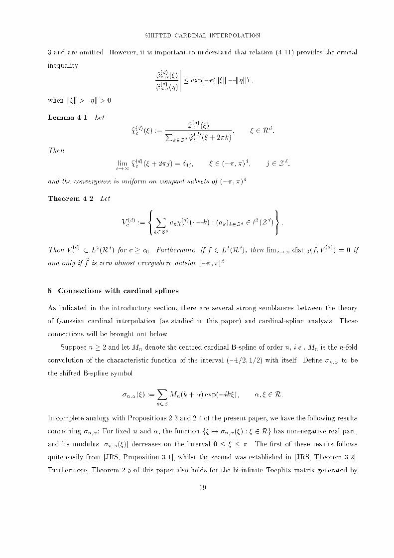
shifted cardinal interpolation3 and are omitted. However, it is important to understand that relation (4.11) provides the crucialinequality ����� b'(d)c;�(�)b'(d)c;�(�)����� � exp[�c(k�k � k�k)];when k�k > k�k > 0.Lemma 4.1. Let b�(d)c (�) := b'(d)c (�)Pk2Zd b'(d)c (� + 2�k) ; � 2 Rd:Then limc!1 b�(d)c (� + 2�j) = �0j ; � 2 (��; �)d; j 2 Zd;and the convergence is uniform on compact subsets of (��; �)d.Theorem 4.2. Let V (d)c := 8<:Xk2Zd ak�(d)c (� � k) : (ak)k2Zd 2 `2(Zd)9=; :Then V (d)c � L2(Rd) for c � c0. Furthermore, if f 2 L2(Rd), then limc!1 dist 2(f; V (d)c ) = 0 ifand only if bf is zero almost everywhere outside [��; �]d.5. Connections with cardinal splinesAs indicated in the introductory section, there are several strong semblances between the theoryof Gaussian cardinal interpolation (as studied in this paper) and cardinal-spline analysis. Theseconnections will be brought out below.Suppose n � 2 and let Mn denote the centred cardinal B-spline of order n, i.e.,Mn is the n-foldconvolution of the characteristic function of the interval (�1=2; 1=2) with itself. De�ne �n;� to bethe shifted B-spline symbol�n;�(�) := Xk2ZMn(k + �) exp(�ik�); �; � 2 R:In complete analogy with Propositions 2.3 and 2.4 of the present paper, we have the following resultsconcerning �n;�: For �xed n and �, the function f� 7! �n;�(�) : � 2 Rg has non-negative real part,and its modulus j�n;�(�)j decreases on the interval 0 � � � �. The �rst of these results followsquite easily from [JRS, Proposition 3.1], whilst the second was established in [JRS, Theorem 3.2].Furthermore, Theorem 2.5 of this paper also holds for the bi-in�nite Toeplitz matrix generated by19

baxter and sivakumarthe shifted B-spline ([M] and [BS]); indeed, the zero structure of the shifted B-spline symbol �n;�(�)is precisely the same as that of the shifted Gaussian symbol G�(�; �) (compare Theorem 2.5 of thispaper with Theorem 2.2 of [S]). As for semi-cardinal interpolation, our Theorem 2.9 for shiftedGaussians is an exact analogue of the corresponding result for shifted B-splines; the latter may bederived as a consequence of [JRS, Proposition 3.1], via [W, Theorem 5].It was shown in [deB, Theorem 1] and [JRS, Theorem 3.4] that for �xed � and n, the evenfunction f� 7! j�n;�(�)j : � 2 Rg decreases on the interval 0 � � � 1=2. We now prove an entirelyanalogous theorem for G�. It is interesting to note that, in stark contrast to the B-spline results,the result for the Gaussian (vide infra) is a simple extension of our earlier analysis.Proposition 5.1. The function f� 7! jG�(�; �)j : � 2 Rg is even, 1-periodic, and decreases on0 � � � 1=2 for every �xed � 2 R and � > 0.Proof. That jG�(�; �)j is an even, 1-periodic function of � is a ready consequence of (2.2). Moreover,the Poisson summation formula impliesG�(�; �) = Xk2ZZ e��(k+�)2e�ik� = (�=�)1=2Xk2Z e�(�+2�k)2=(4�)ei�(�+2�k):Setting � =: 2�� and � := 2��, we obtainG�(�; �) = (�=�)1=2e�i��Xk2Z e�(�2=�)(�+k)2e�ik�= (�=�)1=2e�i��G�(�; �2=�)= (�=�)1=2e�i��e��2�=�#(e�2�2�=�e�i� ; e��2=�);by (2.4), and hence jG�(�; �)j= (�=�)1=2e��2�=�j#(e�2�2�=�e�i� ; e��2=�)j:We have shown in Proposition 2.3 that f� 7! j#(e�2�2�=�e�i� ; e��2=�)j : 0 � � � �g is a decreasingfunction for every �xed � 2 R and � > 0. Therefore the function � 7! jG�(�; �)j decreases on0 � � � 1=2 for every �xed � 2 R and � > 0.A prominent theme in the study of univariate cardinal splines has been that of convergence ofcardinal spline interpolants as the degree of the underlying spline tends to in�nity. Attempts toextend this theory to multivariate splines have led to several interesting results (see, for example,[BHR2, Chapter 5]), including some fascinating connections with problems of tiling [BH]. The studies20

shifted cardinal interpolationreported in Sections 3 and 4 of our paper, as well as those carried out in [B2], reveal that the notionsof \� tending to zero" in Gaussian cardinal interpolation and \c tending to in�nity" in multiquadricinterpolation are natural counterparts of the notion of \degree tending to in�nity" in cardinal-splineanalysis. As a sample, the reader is invited to compare Theorems 3.13 and 4.2 of the present paperwith the main theorem in [BHR1].References[deB] de Boor, C., On the cardinal spline interpolant to eiut, SIAM J. Math. Anal. 7 (1976), 930{941.[B1] Baxter, B. J. C., Norm estimates for inverses of Toeplitz distance matrices, J. Approx. Theory79 (1994), 222{242.[B2] Baxter, B. J. C., On the asymptotic cardinal function of the multiquadric '(r) = (r2 + c2)1=2as c!1, Comput. Math. Applic. 24 (1992), 1{6.[Be] Bellman, R., A brief introduction to Theta functions, Holt, Rinehart and Winston, New York,1961.[Bo] Bollob�as, B., Linear Analysis, Cambridge University Press, 1991.[Bu1] Buhmann, M. D., Multivariate interpolation in odd-dimensional Euclidean spaces using multi-quadrics, Constr. Approx. 6 (1990), 21{34.[Bu2] Buhmann, M. D., Multivariate cardinal interpolation with radial basis functions, Constr. Ap-prox. 6 (1990), 225{256.[Bu3] Buhmann, M. D., New developments in the theory of radial basis function interpolation, inMultivariate approximation: From CAGD to wavelets, K. Jetter and F. I. Utreras (eds.), WorldScienti�c, Singapore, 1993, 35{76.[BH] de Boor, C. and K. H�ollig, Box-spline tilings, Amer. Math. Monthly 98 (1991), 793{802.[BL] Broomhead, D. S. and D. Lowe, Multivariable function interpolation and adaptive networks,Complex Systems 2, 321{355.[BM] Baxter, B. J. C. and C. A. Micchelli, Norm estimates for the `2-inverses of multivariate Toeplitzmatrices, Numerical Algorithms 1 (1994), 103{117.[BS] de Boor, C. and I. J. Schoenberg, Cardinal interpolation and spline functions VIII: The Budan-Fourier theoerm for splines and applications, in Spline functions, Karlsruhe 1975, K. B�ohmer,G. Meinardus and W. Schempp (eds.), Lecture Notes in Mathematics 501, Springer, 1976, 1{79.[BHR1] de Boor, C., K. H�ollig and S. D. Riemenschneider, Convergence of cardinal series, Proc. Amer.Math. Soc. 98 (1986), 457{460.[BHR2] de Boor, C., K. H�ollig and S. D. Riemenschneider, Box Splines, Springer-Verlag, 1993.21

baxter and sivakumar[GS] Grenander, U. and G. Szeg}o, Toeplitz forms, Chelsea, 1984.[H] Hille, E., Analytic Function Theory Vol. II, Ginn and Co., 1962.[JRS] Jetter, K., S. D. Riemenschneider and N. Sivakumar, Schoenberg's exponential Euler splinecurves, Proc. Roy. Soc. Edinburgh 118A (1991), 21{33.[M] Micchelli, C.A., Cardinal L-splines, in Spline functions and applications, S. Karlin et al (eds.),Academic Press, New York, 1976, 203{250.[P] Powell, M. J. D., The theory of radial basis function approximation in 1990, in Advances inNumerical Analysis II, W. A. Light (ed.), Clarendon Press, Oxford, 1992, 106{210.[R] Rahim, R. A., Univariate Hermite interpolation on a shifted lattice using multiquadrics, unpub-lished manuscript, 1992.[S] Sivakumar, N., On univariate cardinal interpolation by shifted splines, Rocky Mountain J. Math.19 (1989), 481{489.[SW] Stein, E. M. and G. Weiss, Introduction to Fourier analysis on Euclidean spaces, PrincetonUniversity Press, Princeton, 1971.[W] Widom, H., Toeplitz Matrices, in Studies in Real and Complex Analysis, I. I. Hirschman (ed.),The Mathematical Association of America, Prentice-Hall, 1965, 179{209.[WW] Whittaker, E. T. and G. N. Watson, A Course of Modern Analysis, Cambridge UniversityPress, Cambridge 1902.

22