On Communication and Collusion∗

Yu Awaya† and Vijay Krishna‡

University of Rochester and Penn State University

August 14, 2015

Abstract

We study the role of communication within a cartel. Our analysis is carriedout in Stigler’s (1964) model of repeated oligopoly with secret price cuts. Firmsobserve neither the prices nor the sales of their rivals. For a fixed discount fac-tor, we identify conditions under which there are equilibria with "cheap talk"that result in near-perfect collusion, whereas all equilibria without such commu-nication are bounded away from this outcome. In our model, communicationimproves monitoring and leads to higher prices and profits.

JEL classification: C73, D43

Keywords: Collusion, communication, repeated games, private monitoring

1 Introduction

Antitrust authorities view any inter-firm communication with concern but despitethis, even well-established cartels meet regularly. In their landmark study of a sugar-refining cartel, Genesove and Mullin (2001) write that cartel members met weekly foralmost a decade! Harrington (2006) too reports on the frequent meetings of cartels inmany industries: Vitamin A and E (weekly or quarterly), citric acid (monthly) andlysine (monthly). Why do cartels find it necessary to meet so often? Court docu-ments and insider accounts reveal that many issues are discussed at such gatherings–demand conditions, costs and yes, sometimes even prices. But an important reasonfirms meet is to monitor each other’s compliance with the collusive agreement. Thisis usually done by exchanging sales data, allowing firms to check that their market

∗We thank Olivier Compte, Joyee Deb, Ed Green and Satoru Takahashi for helpful conversa-tions and various seminar audiences for useful comments. Joseph Harrington and Robert Marshallprovided detailed comments on an earlier draft and enhanced our understanding of antitrust issues.†E-mail: YuAwaya@gmail.com‡E-mail: vkrishna@psu.edu

1

shares are in line with the agreement. Members of the isostatic-graphite cartel enteredtheir sales figures on a pocket calculator that was passed around the table. Only thetotal was displayed, allowing each firm to check its own market share while keeping in-dividual sales confidential. Often data are exchanged not in face-to-face meetings butindirectly through third parties, like trade asssociations, consulting firms or statisticalbureaus. The copper plumbing tubes cartel reported individual sales figures to theWorld Bureau of Metal Statistics which then disseminated these in aggregate form.Many other cartels– for instance, the amino acids and zinc phosphate cartels– usedtrade associations for this purpose.1

It is clear that in these cases cartel members cannot ascertain each other’s salesdirectly; otherwise, there would be no need for firms to report these figures. Self-reported sales numbers, however, are diffi cult to verify and firms have the incentiveto under-report these. Recognizing this, the lysine cartel even resorted to auditing itsmembers. This was only moderately successful– a leading firm, Ajinomoto, was stillable to hide its actual sales. Given that the data provided by firms cannot be verifiedwhat is the point of having them report these? Can such "cheap-talk" communicationreally help firms monitor each other?In this paper, we study how unverifiable communication about past sales can

indeed facilitate collusion. We adopt, and adapt, Stigler’s (1964) classic oligopolymodel of secret price cuts in a repeated setting– firms cannot observe each other’sprices nor can they observe each other’s sales. Each firm observes only its ownsales and because of demand shocks, both common and idiosyncratic, these are noisysignals of other firms’actions. Absent any communication, such imperfect monitoringlimits the potential for collusive behavior because– and this was Stigler’s point–deviations from a collusive agreement cannot be detected with confidence. We show,however, that if firms are able to exchange sales information, then collusive outcomescan be sustained. We study situations where the correlation in firms’sales is sensitiveto prices. Precisely, it is high when the difference in firms’prices is small– say, whenboth firms charge close to monopoly prices– and decreases when the difference islarge– say, because of a unilateral price cut.2 For analytic convenience, we supposethat the relationship between sales and prices is governed by log-normal distributions,independently over time.We show that in the statistical environment outlined above, reports of past sales

allow firms to better monitor each other. The information communicated is not onlyunverifiable but also payoff irrelevant– it has no direct effects on current or futureprofits. Our main result is3

THEOREM. For any high but fixed discount factor, when the monitoring is noisy

1Details of these and other cartel cases can be found in Harrington (2006) and Marshall andMarx (2012).

2This can arise quite naturally, for example, in a Hotelling-type model with random transportcosts (see Section 2).

3A formal statement of the result is in Section 5.

2

but sensitive enough, there is an equilibrium with communication whose profits arestrictly greater than those from any equilibrium without communication.

The argument underlying our main result is divided into two steps. The firsttask is to find an effective bound for the maximum equilibrium profits that canbe achieved in the absence of any communication. In Proposition 1 we develop abound on equilibrium profits by using a very simple necessary condition– a deviatingstrategy in which a firm permanently cuts its price to an unchanging level shouldnot be profitable. This deviation is, of course, rather naive– the deviating firm doesnot take into account what the other firm knows or does. We show, however, thateven this minimal requirement can provide an effective bound when the relationshipbetween prices and sales is rather noisy relative to the discount factor. For a fixeddiscount factor, as sales become increasingly noisy, the bound becomes tighter.The second task is to show that the bound developed earlier can be exceeded

with communication. We directly construct an equilibrium in which firms exchange(coarse) sales reports in every period (see Proposition 2). Firms charge monopolyprices and report their sales truthfully. As long as the reported sales of the firms–whether high or low– are similar, monopoly prices are maintained. If the reportedsales are significantly different– say, one firm reports high sales while the other reportslow– a price war is triggered. These strategies form an equilibrium because whenfirms charge monopoly prices, their sales are highly correlated and so the likelihoodthat their truthful reports will agree is also high. If a firm cuts its price, salesbecome less correlated and so it cannot accurately predict its rival’s sales. Even ifthe deviating firm strategically tailors its report, the likelihood of an agreement islow. Thus a strategy in which differing sales reports lead to non-cooperation is aneffective deterrent. In this way, cheap-talk communication allows firms to monitoreach other more effectively.We emphasize that the analysis in this paper is of a different nature than that

underlying the so-called "folk theorems" (see Mailath and Samuelson, 2006). Theseshow that for a fixed monitoring structure, as players become increasingly patient,near-perfect collusion can be achieved in equilibrium. In this paper, we keep the dis-count factor fixed and change the monitoring structure in a way that communicationimproves profits.

1.0.1 Real-world Cartels

Some key features of our model echo aspects of real-world cartel behavior. First,monitoring is imperfect and diffi cult. Second, the purpose of communication is toovercome monitoring diffi culties and it is unverifiable. Third, communication allowsfirms to base their future behavior on relative sales– market shares– rather than theabsolute level of sales.The diffi culties firms face in monitoring each other have been well-documented.

Secret price cuts are hard to track. In the famous Trenton Potteries case, first-quality

3

products were invoiced as being of second quality and so sold at a discount. In thesugar refining case, a firm included some shipping expenses in the quoted price. Ineach case, other members of the cartel discovered this "price cut" only with diffi culty.Clark and Houde (2014) study the internal functioning of a gasoline distribution

cartel via recordings of telephone conversations. They use a "natural experiment"– apublic announcement of an investigation that led to a cessation of all communication–to deduce that higher prices and profits result when firms communicate. Clark andHoude (2014) find that the communication helped the members to both coordinatepricing and to monitor each other. Harrington (2006) and Marshall and Marx (2012)study numerous cartels and how these functioned. Again, regular communication formonitoring purposes seems to be a common feature of cartels in many industries.Often the verity of what is communicated must be inferred. Indeed, Genesove andMullin (2001, p. 389) write that the meetings of the sugar-refining cartel often served"as a court in which an accused firm might prove its innocence, in some cases onfactual, in others on logical, grounds." [Emphasis added.]Harrington (2006) writes that the monitoring of sales is even more important

than the monitoring of prices. As mentioned above, firms are often informed onlyabout total industry sales– via a calculator or a trade association– because these aresuffi cient for firms to calculate their own market shares. In our model too, a pricewar is triggered by relative sales (market shares) and not by the absolute level ofsales. If all firms experience low sales– and so shares are not too far off– then this isattributed to adverse market conditions and the firms continue to collude. Implicitly,a firm that experiences low sales cares about the reason that its sales are low andnot just the fact that they are low. Genesove and Mullin (2001) recount an episodein which the president of a Western firm threatened a price war unless it could beconvinced that its low sales were not caused by the actions of Eastern refiners. Noticethat this sort of behavior would not be possible without communication. A firm thatonly knew its own sales would be unable to infer the reason why they were low.

1.0.2 Other Models of Collusion

The application of the theory of repeated games to understand collusion goes backat least to Friedman (1971). His model assumes that all past actions are commonlyobserved without any noise. Under such perfect monitoring, given any fixed discountfactor, the set of subgame perfect equilibrium payoffs with and without communica-tion is the same– there is nothing useful to communicate. Collusion with imperfectmonitoring was studied by Green and Porter (1984) in a model of repeated quantitycompetition with noisy demand. Monitoring is imperfect because firms do not ob-serve each others’output but rather only the market price. Since all firms observethe same noisy signal (the common price), this situation is referred to as one of pub-lic monitoring. Again given any fixed discount factor, the set of profits from (purestrategy) public perfect equilibria– in which firms’strategies depend only on the his-

4

tory of past prices– with and without communication is also the same. Green andPorter (1984) show that with suffi ciently low discounting, public perfect equilibria areenough to sustain collusion.4 Our model is one of private monitoring– different firmsobserve different noisy signals (their own sales). As we show, in this environment,communication enlarges the set of equilibria. In both models, the firms are necessar-ily subject to a "type II" error when colluding– price wars are triggered even if noone has deviated. In the Green and Porter (1984) model, firms cannot distinguishbetween a deviation and an aggregate market shock– both lead to lower profits andresult in price wars. In our model, communication allows firms to distinguish betweenthe two– one leads to lower sales for all while the other leads to a discrepancy in salesand market shares. As mentioned above, only the latter triggers a punishment.In our model, communication improves monitoring and, by enhancing the possi-

bility of collusion, reduces welfare. Of course, not all communication need be welfarereducing. It can play a benign, even beneficial, role in some circumstances by allowingfirms to share economically valuable information about demand or cost conditions.Indeed, the courts have long recognized this possibility and opined that such informa-tion sharing "... can hardly be deemed a restraint of commerce ... or in any respectunlawful."5 Economists and legal scholars have elaborated this argument (Shapiro,1986 and Carlton, Gertner and Rosenfield, 1996). The sharing of privately knowncosts via cheap talk is studied in a repeated-game model by Athey and Bagwell (2001).They show that, for moderate discounting, cheap-talk communication increases prof-its. The channel through which this occurs is quite different from ours, however.The Athey and Bagwell (2001) model is one of perfect monitoring but incompletepayoff-relevant information (costs). Communication allows firms to allocate greatermarket shares in favor of low cost firms and these cost savings are the source of al-most all of the profit gains. Thus, communication actually has social benefits– theresulting production effi ciencies increase welfare. By contrast, our model is one ofimperfect monitoring but complete information. Communication improves monitor-ing and this is the only source of profit gains. Now, communication has no socialbenefits– the resulting high prices reduce welfare. Another way to see the differenceis by considering how a "planner" who can dictate the prices that firms charge wouldimplement collusive outcomes in the two models. In the Athey and Bagwell (2001)model, such a planner must elicit the privately known cost information in order toimplement maximally collusive outcomes. The resulting mechanism design problemnecessitates communication. It then seems clear that in the absence of a planner,colluding firms would need to communicate with each other as well. In our model,however, there is no need to communicate any information to such a planner– he/shecan simply dictate that firms charge the monopoly price. In this case, the fact thatin the absence of a planner, maximally collusive outcomes can only be achieved with

4The effect of introducing communication in such a model has been studied in a paper by Rahman(2014), which we discuss later.

5Areeda and Kaplow (1988, pp. 337-338).

5

communication is our main finding. We believe that we are the first to establish thatcheap-talk communication about payoff irrelevant information can aid collusion.The remainder of the paper is organized as follows. The next section outlines

the nature of the market. Section 3 analyzes the repeated game without communi-cation whereas Section 4 does the same with. The findings of the earlier sectionsare combined in Section 5 to derive the main result. We also calculate explicitly thegains from communication in an example with linear demands. Omitted proofs arecollected in an Appendix.

2 The Market

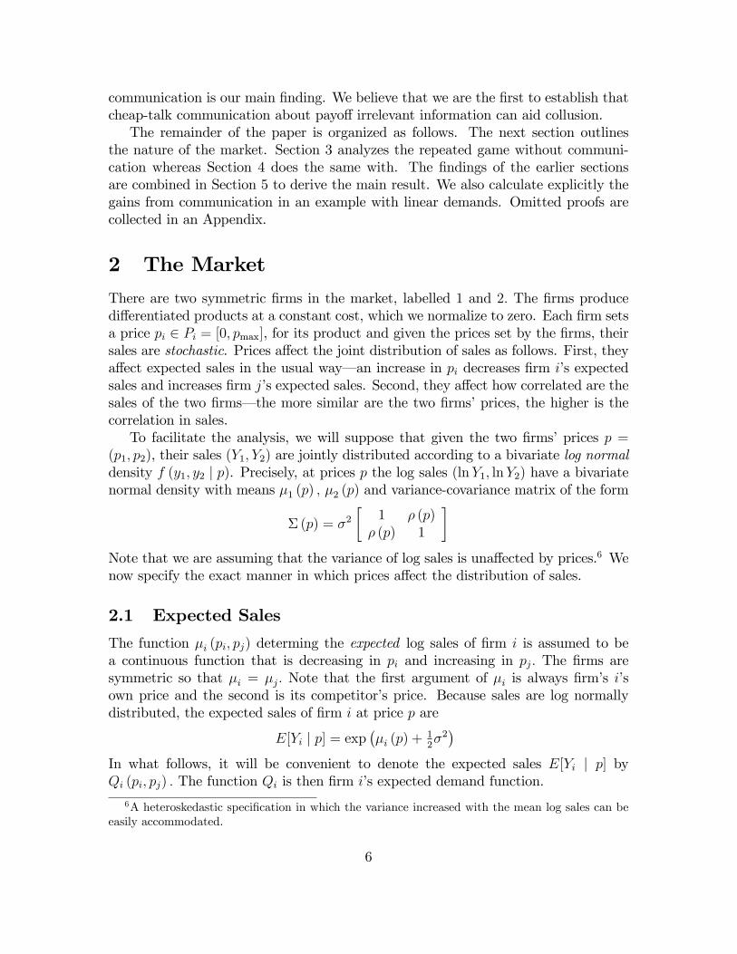
There are two symmetric firms in the market, labelled 1 and 2. The firms producedifferentiated products at a constant cost, which we normalize to zero. Each firm setsa price pi ∈ Pi = [0, pmax], for its product and given the prices set by the firms, theirsales are stochastic. Prices affect the joint distribution of sales as follows. First, theyaffect expected sales in the usual way– an increase in pi decreases firm i’s expectedsales and increases firm j’s expected sales. Second, they affect how correlated are thesales of the two firms– the more similar are the two firms’prices, the higher is thecorrelation in sales.To facilitate the analysis, we will suppose that given the two firms’prices p =

(p1, p2), their sales (Y1, Y2) are jointly distributed according to a bivariate log normaldensity f (y1, y2 | p). Precisely, at prices p the log sales (lnY1, lnY2) have a bivariatenormal density with means µ1 (p) , µ2 (p) and variance-covariance matrix of the form

Σ (p) = σ2

[1 ρ (p)

ρ (p) 1

]Note that we are assuming that the variance of log sales is unaffected by prices.6 Wenow specify the exact manner in which prices affect the distribution of sales.

2.1 Expected Sales

The function µi (pi, pj) determing the expected log sales of firm i is assumed to bea continuous function that is decreasing in pi and increasing in pj. The firms aresymmetric so that µi = µj. Note that the first argument of µi is always firm’s i’sown price and the second is its competitor’s price. Because sales are log normallydistributed, the expected sales of firm i at price p are

E[Yi | p] = exp(µi (p) + 1

2σ2)

In what follows, it will be convenient to denote the expected sales E[Yi | p] byQi (pi, pj) . The function Qi is then firm i’s expected demand function.

6A heteroskedastic specification in which the variance increased with the mean log sales can beeasily accommodated.

6

-

6

lnY1

lnY2

µ2

µ

µ µ1

p1 = p2

p1 < p2

rr

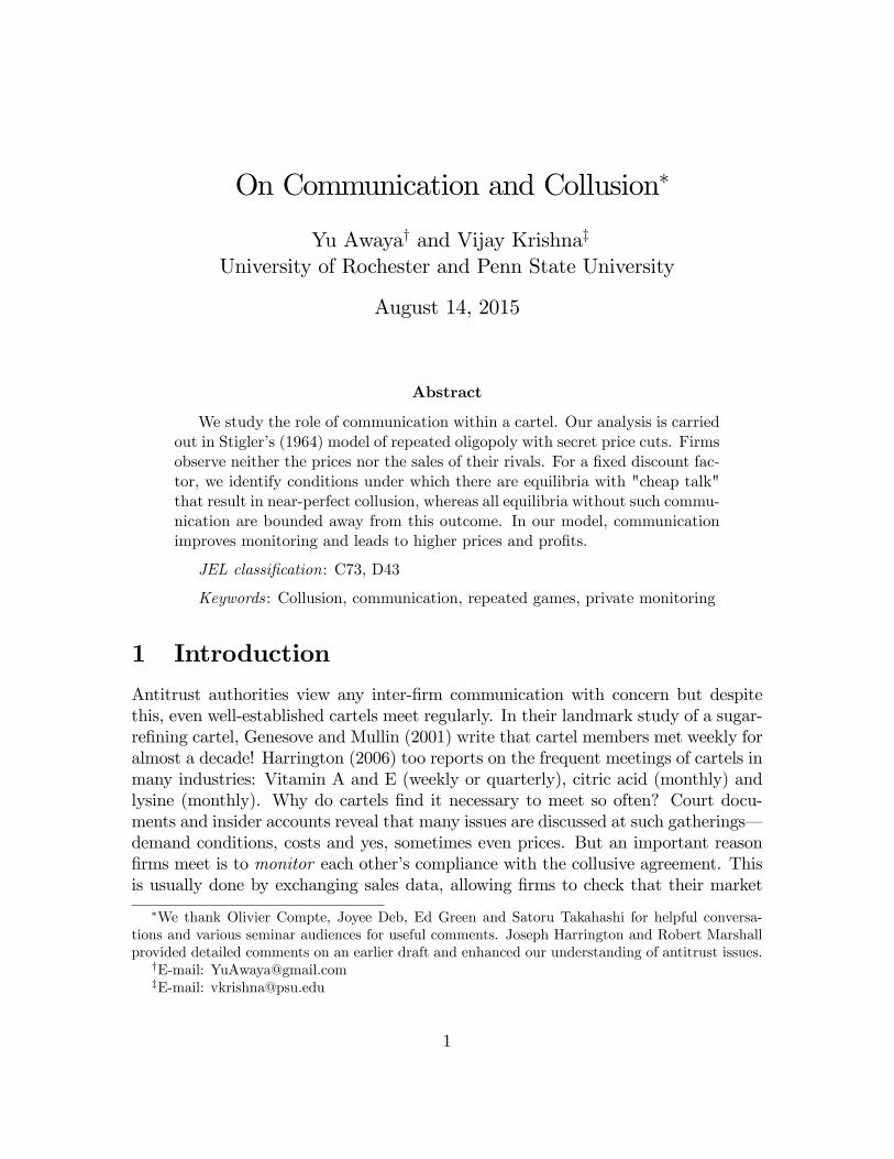
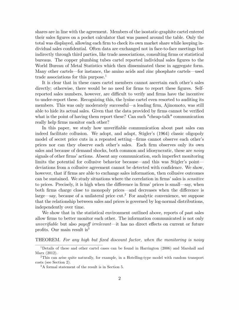
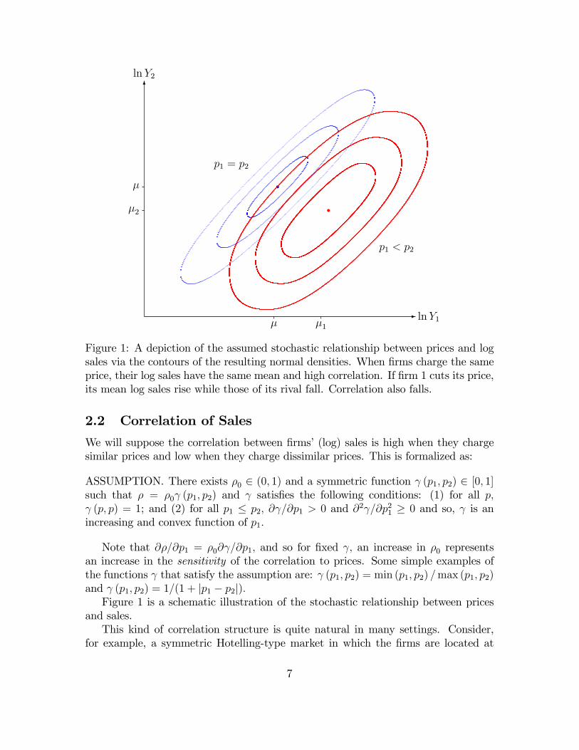
Figure 1: A depiction of the assumed stochastic relationship between prices and logsales via the contours of the resulting normal densities. When firms charge the sameprice, their log sales have the same mean and high correlation. If firm 1 cuts its price,its mean log sales rise while those of its rival fall. Correlation also falls.

2.2 Correlation of Sales

We will suppose the correlation between firms’(log) sales is high when they chargesimilar prices and low when they charge dissimilar prices. This is formalized as:

ASSUMPTION. There exists ρ0 ∈ (0, 1) and a symmetric function γ (p1, p2) ∈ [0, 1]such that ρ = ρ0γ (p1, p2) and γ satisfies the following conditions: (1) for all p,γ (p, p) = 1; and (2) for all p1 ≤ p2, ∂γ/∂p1 > 0 and ∂2γ/∂p2

1 ≥ 0 and so, γ is anincreasing and convex function of p1.

Note that ∂ρ/∂p1 = ρ0∂γ/∂p1, and so for fixed γ, an increase in ρ0 representsan increase in the sensitivity of the correlation to prices. Some simple examples ofthe functions γ that satisfy the assumption are: γ (p1, p2) = min (p1, p2) /max (p1, p2)and γ (p1, p2) = 1/(1 + |p1 − p2|).Figure 1 is a schematic illustration of the stochastic relationship between prices

and sales.This kind of correlation structure is quite natural in many settings. Consider,

for example, a symmetric Hotelling-type market in which the firms are located at

7

different points on the line and consumers have identical but random "transport"costs. First, consider the case where the two firms charge very similar prices. Inthis case, their sales are similar– roughly, they split the market– no matter whatthe realized transport costs are. In other words, when firms charge similar prices,their sales are highly correlated. Next, consider the case where the two firms’pricesare dissimilar, say, firm 1’s price is much lower than firm 2’s price. When transportcosts are high, consumers are not that price sensitive and so the firms’realized salesare rather similar. But when transports costs are low, consumers are rather pricesensitive and so firm 1’s sales are much higher than firm 2’s sales. In other words,when firms charge dissimilar prices, the correlation between their sales is low. Ofcourse, the same kind of reasoning applies if we substitute search costs for transportcosts.Another setting in which the kind of correlation structure postulated above arises

is the "random utility" model for discrete choice, widely used as the basis of manyempirical industrial organization studies. In such a specification, consumers’utilityis assumed to have both common and idiosyncratic components and the commoncomponent plays a role not unlike that of transport costs in the Hotelling model.Again, consider first the case where firms charge similar prices. Now, regardlessof the realization of the common component, their sales are similar and so highlycorrelated. But when the firms charge different prices, how close their sales aredepends on the realization of the common component of utility. When the commoncomponent is high, prices are not that important for consumers and so the sales of thetwo firms will be relatively similar. When the common component is low, however,price differences become important, the lower-priced firm will experience much highersales than its rival, and so the two firms’sales will be dissimilar. Overall, this meansthat the correlation between their sales is lower.

2.3 One-shot Game

Firms maximize their expected profits:

πi (pi, pj) = piQi (pi, pj)

and we suppose that πi is strictly concave in pi.7

Let G denote the one-shot game where the firms choose prices pi and pj and theexpected profits are given by πi (pi, pj) . Under the assumptions made above, thereexists a symmetric Nash equilibrium (pN , pN) of G and let πN be the resulting profitsof a firm.8

Suppose that (pM , pM) is the unique solution to the monopolist’s problem:

maxpi,pj

∑i

πi (pi, pj)

7In terms of the primitives, this is guaranteed if µi is suffi ciently concave.8If the one-shot game has multiple symmetric Nash equilibria, let (pN , pN ) denote the one with

the lowest equilibrium profits.

8

and let πM be the resulting profits per firm. We assume that monopoly pricing(pM , pM) is not a Nash equilibrium. For technical reasons we will also assume that afirm’s expected sales are bounded away from zero.

3 Collusion without Communication

Let Gδ (f) denote the infinitely repeated game in which firms use the discount factorδ < 1 to evaluate profit streams. Time is discrete. In each period, firms choose pricespi and pj and given these prices, their sales are realized according to f as describedabove. As in Stigler (1964), each firm i observes only its own realized sales yi; itobserves neither j’s price pj nor j’s sales yj. We will refer to f as the monitoringstructure.Let ht−1

i =(p1i , y

1i , p

2i , y

2i , ..., p

t−1i , yt−1

i

)denote the private history observed by firm

i after t− 1 periods of play and let H t−1i denote the set of all private histories of firm

i. In period t, firm i chooses its prices pti knowing ht−1i and nothing else.

A strategy si for firm i is a collection of functions (s1i , s

2i , ...) such that s

ti : H t−1

i →∆ (Pi) , where ∆ (Pi) is the set of distributions over Pi. Thus, we are allowing for thepossibility that firms may randomize. Of course, since H0

i is null, s1i ∈ ∆ (Pi) . A

strategy profile s is simply a pair of strategies (s1, s2). A Nash equilibrium of Gδ (f)is strategy profile s such that for each i, the strategy si is a best response to sj.The main result of this section provides an upper bound to the joint profits of the

firms in any Nash equilibrium of the repeated game without communication.9 Thetask is complicated by the fact that there is no known characterization of the set ofequilibrium payoffs of a repeated game with private monitoring. Because the playersin such a game observe different histories– each firm knows only its own past pricesand sales– such games lack a straightforward recursive structure and the kinds oftechniques available to analyze equilibria of repeated games with public monitoring(as in the work of Abreu, Pearce and Stacchetti, 1990) cannot be used here.Instead, we proceed as follows. Suppose we want to determine whether there is

a Nash equilibrium of Gδ (f) such that the sum of firms’discounted average profitsare within ε of those of a monopolist, that is, 2πM . If there were such an equilibrium,then both firms must set prices close to the monopoly price pM often (or equivalently,with high probability). Now consider a secret price cut by firm 1 to p, the static bestresponse to pM . Such a deviation is profitable today because firm 2’s price is closeto pM with high probability. How this affects firm 2’s future actions depends on thequality of monitoring, that is, how much firm 1’s price cut affects the distributionof 2’s sales. If the quality of monitoring is poor, firm 1 can keep on deviating to pwithout too much fear of being punished. In other words, a firm has a profitabledeviation, contradicting that there were such an equilibrium.This reasoning shows that the resulting bound on Nash equilibrium profits depends

9Of course, the bound so derived applies to any refinement of Nash equilibrium as well.

9

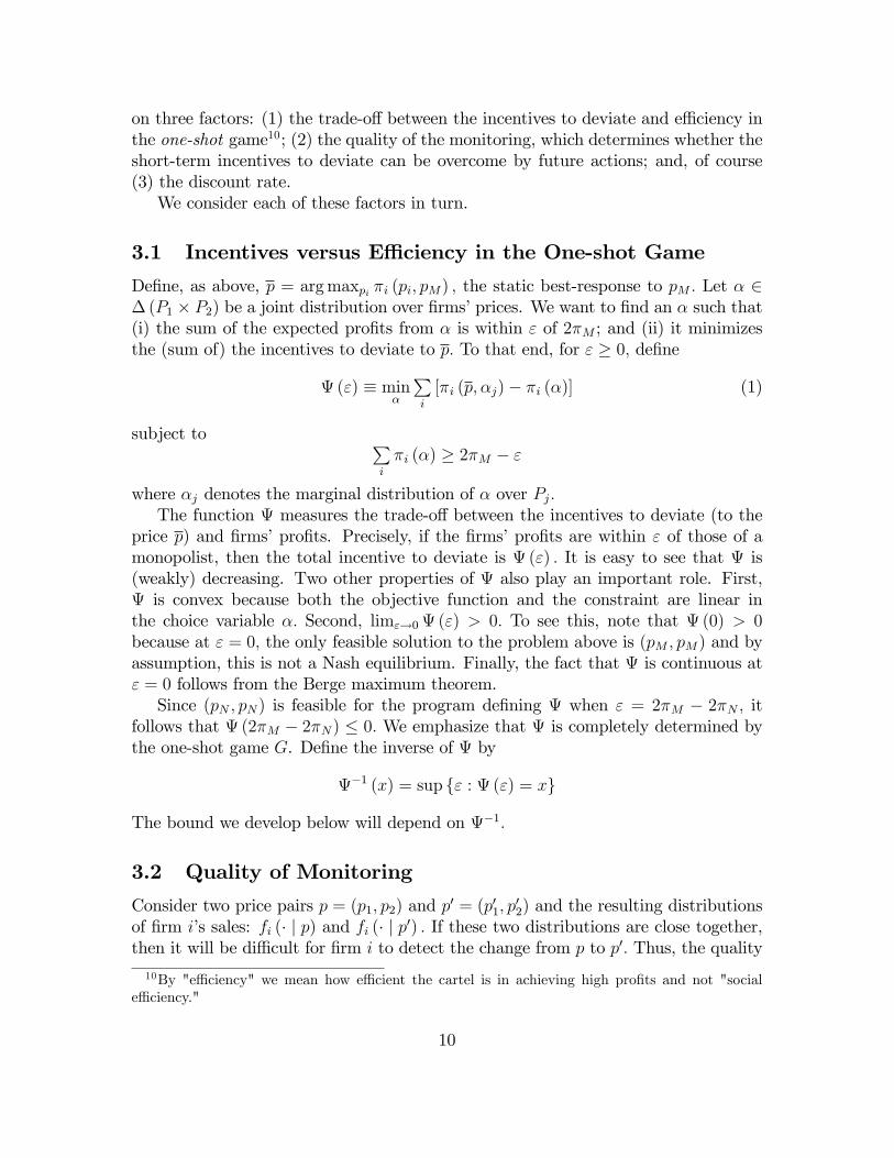
on three factors: (1) the trade-off between the incentives to deviate and effi ciency inthe one-shot game10; (2) the quality of the monitoring, which determines whether theshort-term incentives to deviate can be overcome by future actions; and, of course(3) the discount rate.We consider each of these factors in turn.

3.1 Incentives versus Effi ciency in the One-shot Game

Define, as above, p = arg maxpi πi (pi, pM) , the static best-response to pM . Let α ∈∆ (P1 × P2) be a joint distribution over firms’prices. We want to find an α such that(i) the sum of the expected profits from α is within ε of 2πM ; and (ii) it minimizesthe (sum of) the incentives to deviate to p. To that end, for ε ≥ 0, define

Ψ (ε) ≡ minα

∑i

[πi (p, αj)− πi (α)] (1)

subject to ∑i

πi (α) ≥ 2πM − ε

where αj denotes the marginal distribution of α over Pj.The function Ψ measures the trade-off between the incentives to deviate (to the

price p) and firms’profits. Precisely, if the firms’profits are within ε of those of amonopolist, then the total incentive to deviate is Ψ (ε) . It is easy to see that Ψ is(weakly) decreasing. Two other properties of Ψ also play an important role. First,Ψ is convex because both the objective function and the constraint are linear inthe choice variable α. Second, limε→0 Ψ (ε) > 0. To see this, note that Ψ (0) > 0because at ε = 0, the only feasible solution to the problem above is (pM , pM) and byassumption, this is not a Nash equilibrium. Finally, the fact that Ψ is continuous atε = 0 follows from the Berge maximum theorem.Since (pN , pN) is feasible for the program defining Ψ when ε = 2πM − 2πN , it

follows that Ψ (2πM − 2πN) ≤ 0. We emphasize that Ψ is completely determined bythe one-shot game G. Define the inverse of Ψ by

Ψ−1 (x) = sup {ε : Ψ (ε) = x}

The bound we develop below will depend on Ψ−1.

3.2 Quality of Monitoring

Consider two price pairs p = (p1, p2) and p′ = (p′1, p′2) and the resulting distributions

of firm i’s sales: fi (· | p) and fi (· | p′) . If these two distributions are close together,then it will be diffi cult for firm i to detect the change from p to p′. Thus, the quality

10By "effi ciency" we mean how effi cient the cartel is in achieving high profits and not "socialeffi ciency."

10

of monitoring can be measured by the maximum "distance" between any two suchdistributions. In what follows, we use the so-called total variation metric to measurethis distance. Since f is symmetric, the quality of monitoring is the same for bothfirms.

Definition 1 The quality of a monitoring structure f is defined as

η = maxp,p′‖fi (· | p)− fi (· | p′)‖TV

where fi is the marginal of f on Yi and ‖g − h‖TV denotes the total variation distancebetween g and h.11

It is important to note that the quality of monitoring depends only on themarginaldistributions fi (· | p) over i’s sales and not on the joint distributions of sales f (· | p) .In particular, the fact that the marginal distributions fi (· | p) and fi (· | p′) are close–η is small– does not imply that the underlying joint distributions f (· | p) and f (· | p′)are close. Because of symmetry, η is the same for both firms. When f (· | p) is abivariate log normal, η can be explicitly determined as

η = 2Φ(

∆µmax2σ

)− 1 (2)

where Φ is the cumulative distribution function of a univariate standard normal and∆µmax = maxp,p′ | lnQi(pi, pj)−lnQi(p

′i, p′j)| is the maximum possible difference in log

expected sales. As σ increases, η decreases and goes to zero as σ becomes arbitrarilylarge.

3.3 A Bound on Profits

The main result of this section, stated below, develops a bound on Nash equilibriumprofits when there is no communication. An important feature of the bound is thatit is independent of any correlation between firms’ sales and depends only on themarginal distribution of sales.

Proposition 1 In any Nash equilibrium of the repeated game without communica-tion, the average profits

π1 + π2 ≤ 2πM −Ψ−1(

4πη δ2

1−δ

)(3)

where π = maxpj πi (p, pj) and η is the quality of monitoring.

11The total variation distance between two densities g and h on X is defined as ‖g − h‖TV =12

∫X|g (x)− h (x)| dx.

11

-

6

0

(πM , πM)

(πN , πN)

π1

π2

Ψ−1����

���

s

s

@@@@@@@@@@@@@@@@@@

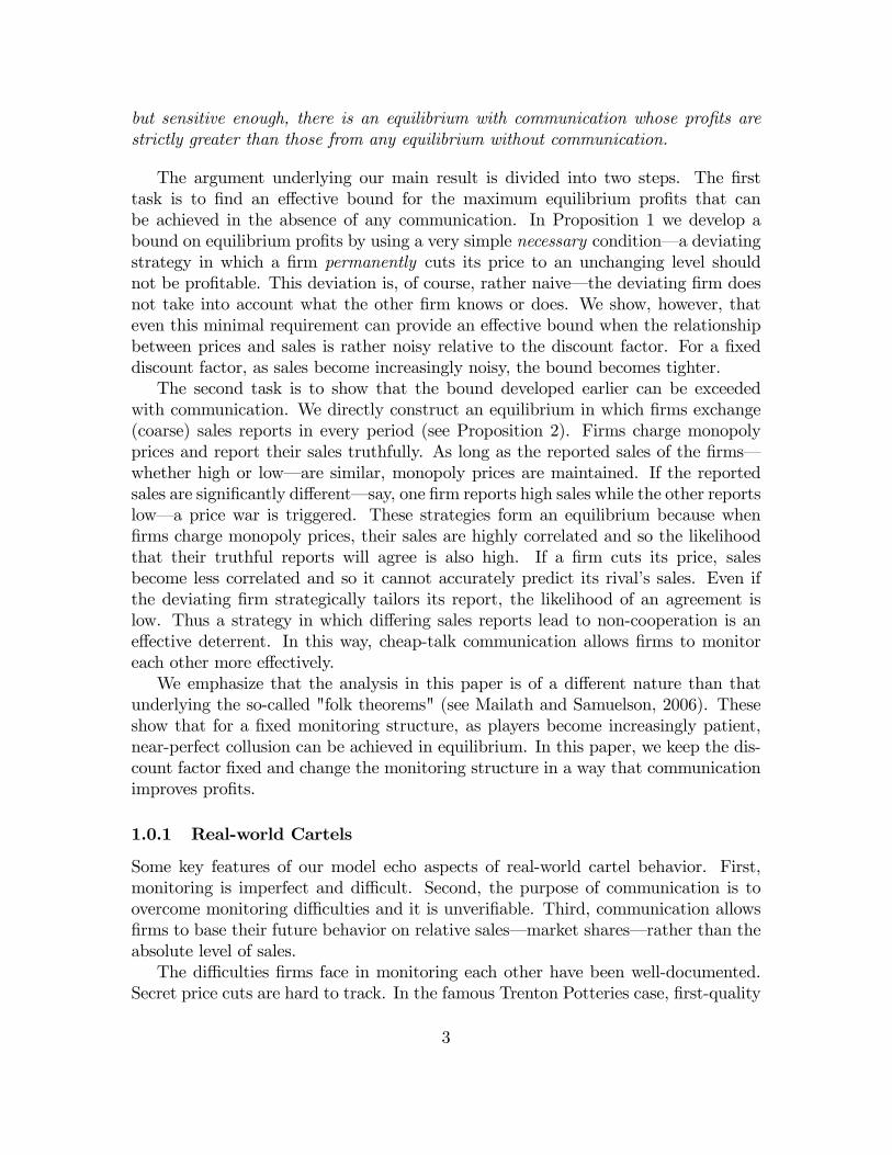
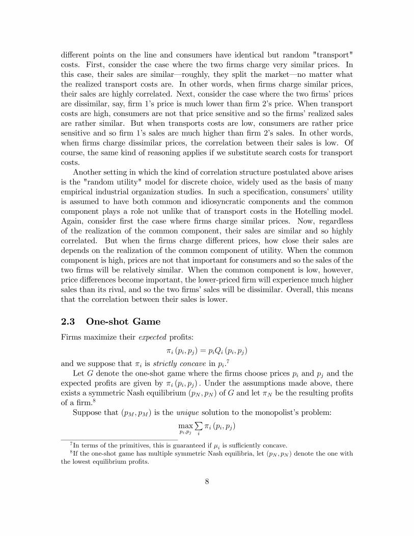
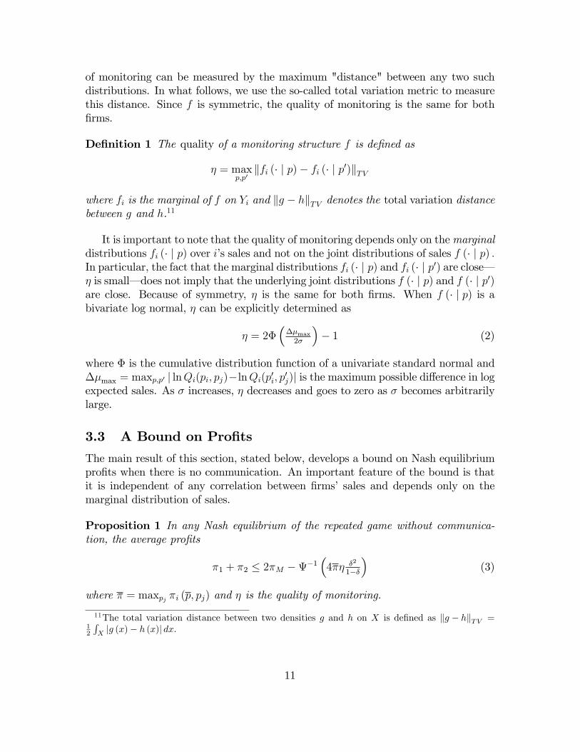
Figure 2: The set of feasible profits of the two firms and the position of the no-communication bound is depicted. The bound lies between monopoly and one-shotNash profits and its size depends on the demand structure, the discount factor andthe monitoring quality.

Before embarking on a formal proof of Proposition 1 it is useful to outline the mainideas (see Figure 3 for an illustration). A necessary condition for a strategy profile sto be an equilibrium is that a deviation by firm 1 to a strategy s1 in which it alwayscharges p not be profitable. This is done in two steps. First, we consider a fictitioussituation in which firm 1 assumes that firm 2 will not respond to its deviation. Thehigher the equilibrium profits, the more profitable would be the proposed deviation inthe fictitious situation– this is exactly the effect the function Ψ captures in the one-shot game and Lemma A.1 shows that Ψ captures the same effect in the repeatedgame as well. Second, when the monitoring is poor– η is small– firm 2’s actionscannot be very responsive to the deviation and so the fictitious situation is a goodapproximation for the true situation. Lemma A.5 measures precisely how good thisapproximation is and quite naturally this depends on the quality of monitoring andthe discount factor. Notice that profits both from the candidate equilibrium and fromthe play after the deviation are evaluated in ex ante terms.Observe that if we fix the quality of monitoring η and let the discount factor δ

approach one, then the bound becomes trivial (since limδ→1 Ψ−1(4πηδ2/ (1− δ)

)= 0)

and so is consistent with Sugaya’s (2013) folk theorem. On the other hand, if we fixthe discount factor δ and decrease the quality of monitoring η, the bound convergesto 2πM − Ψ−1 (0) < 2πM and is effective. One may reasonably conjecture that if

12

there were "zero monitoring" in the limit, that is, if η → 0, then no collusion wouldbe possible. But in fact 2πN < 2πM − Ψ−1 (0) so that even with zero monitoring,Proposition 1 does not rule out the presence of collusive equilibria. This is consistentwith the finding of Awaya (2014b).12

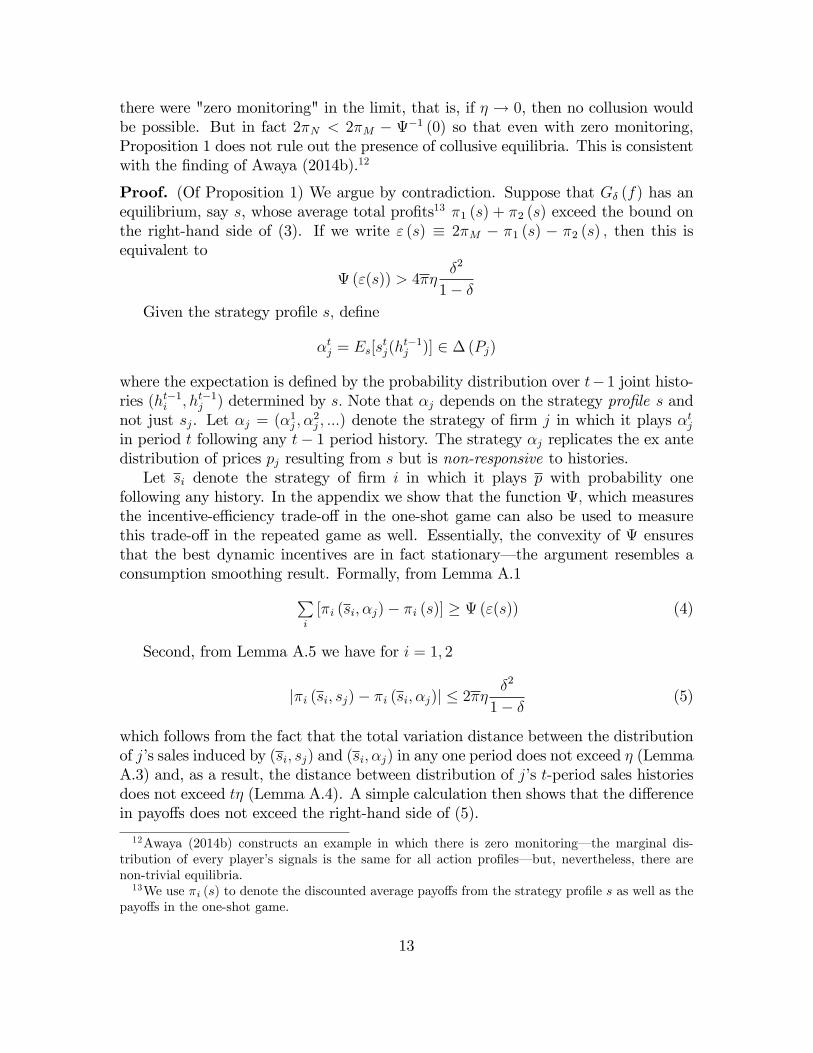
Proof. (Of Proposition 1) We argue by contradiction. Suppose that Gδ (f) has anequilibrium, say s, whose average total profits13 π1 (s) + π2 (s) exceed the bound onthe right-hand side of (3). If we write ε (s) ≡ 2πM − π1 (s) − π2 (s) , then this isequivalent to

Ψ (ε(s)) > 4πηδ2

1− δGiven the strategy profile s, define

αtj = Es[stj(h

t−1j )] ∈ ∆ (Pj)

where the expectation is defined by the probability distribution over t−1 joint histo-ries (ht−1

i , ht−1j ) determined by s. Note that αj depends on the strategy profile s and

not just sj. Let αj = (α1j , α

2j , ...) denote the strategy of firm j in which it plays αtj

in period t following any t− 1 period history. The strategy αj replicates the ex antedistribution of prices pj resulting from s but is non-responsive to histories.Let si denote the strategy of firm i in which it plays p with probability one

following any history. In the appendix we show that the function Ψ, which measuresthe incentive-effi ciency trade-off in the one-shot game can also be used to measurethis trade-off in the repeated game as well. Essentially, the convexity of Ψ ensuresthat the best dynamic incentives are in fact stationary– the argument resembles aconsumption smoothing result. Formally, from Lemma A.1∑

i

[πi (si, αj)− πi (s)] ≥ Ψ (ε(s)) (4)

Second, from Lemma A.5 we have for i = 1, 2

|πi (si, sj)− πi (si, αj)| ≤ 2πηδ2

1− δ (5)

which follows from the fact that the total variation distance between the distributionof j’s sales induced by (si, sj) and (si, αj) in any one period does not exceed η (LemmaA.3) and, as a result, the distance between distribution of j’s t-period sales historiesdoes not exceed tη (Lemma A.4). A simple calculation then shows that the differencein payoffs does not exceed the right-hand side of (5).

12Awaya (2014b) constructs an example in which there is zero monitoring– the marginal dis-tribution of every player’s signals is the same for all action profiles– but, nevertheless, there arenon-trivial equilibria.13We use πi (s) to denote the discounted average payoffs from the strategy profile s as well as the

payoffs in the one-shot game.

13

Combining (4) and (5), we have∑i

(πi(si, sj)− πi(s)) =∑i

(πi(si, αj)− πi(s)) +∑i

(πi(si, sj)− πi(si, αj))

≥∑i

(πi(si, αj)− πi(s))−∑i

|πi(si, sj)− πi(si, αj)|

≥ Ψ (ε(s))− 4πηδ2

1− δ

which is strictly positive. But this means that at least one firm has a profitabledeviation, contradicting the assumption that s is an equilibrium.This completes the proof.In a recent paper, Pai, Roth and Ullman (2014) also provide a bound on equi-

librium payoffs that is effective when monitoring is poor. They derive necessaryconditions for an equilibrium by considering "one-shot" deviations in which a playercheats in one period and then resumes equilibrium play. Pai et al.’s bound is basedon how the joint distribution of the private signals is affected by players’actions.In games with private monitoring, "one-shot" deviations affect the deviating play-

ers’beliefs about the other player’s signals thereafter and so affect his subsequent(optimal) play. The optimal play, quite naturally, exploits any correlation in signals.The deviation we consider– a permanent price cut– is rather naive but has the fea-ture that future play, while suboptimal, is straightforward. This renders unnecessaryany conjectures about the future behavior of the other firm and so our bound does notdepend on any correlation between signals (sales); it is based solely on the marginaldistributions.When we consider communication in the next section, we will exploit the corre-

lation of signals to construct an equilibrium whose profits exceed our bound (Propo-sition 2 below). The fact that correlation can vary while keeping the marginal dis-tributions fixed is key to isolating the effects of communication. The bound ob-tained by Pai, et al. (2014) applies to both forms of collusion– with and with-out communication– and cannot distinguish between the two. Sugaya and Wolitzky(2015) also provide a bound but one that is based on entirely different ideas. For afixed discount factor, they ask which monitoring structure yields the highest equilib-rium profits. This, of course, then identifies a bound that applies across all monitoringstructures. But this method, while quite general, again cannot distinguish betweenthe two settings.

4 Collusion with Communication

We now turn to a situation in which firms can, in addition to setting prices, com-municate with each other in every period, sending one of a finite set of messages toeach other. The sequence of actions in any period is as follows: firms set prices,

14

receive their private sales information and then simultaneously send messages to eachother. Messages are costless– the communication is "cheap talk"– and are transmit-ted without any noise. The communication is unmediated.Formally, there is a finite set of messages Mi for each firm and that each Mi

contains at least two elements. A t− 1 period private history of firm i now consistsof the complete list of its own prices and sales as well as the list of all messages sentand received. Thus a private history is now of the form

ht−1i =

(pτi , y

τi ,m

τi ,m

τj

)t−1

τ=1

and the set of all such histories is denoted by H t−1i . A strategy for firm i is now a pair

(si, ri) where si = (s1i , s

2i , ...), the pricing strategy, and ri = (r1

i , r2i , ...) , the reporting

strategy, are collections of functions: sti : H t−1i → ∆ (Pi) and rti : H t−1

i × Pi × Yi →∆ (Mi) .Call the resulting infinitely repeated game with communication Gcom

δ (f) . A se-quential equilibrium of Gcom

δ (f) is a strategy profile (s, r) such that for each i andevery private history ht−1

i , the continuation strategy of i following ht−1i , denoted by

(si, ri) |ht−1i, is a best response to E[(sj, rj) |ht−1j

| ht−1i ].14

4.1 Equilibrium Strategies

Monopoly pricing will be sustained using a grim trigger pricing strategy togetherwith a threshold sales-reporting strategy in a manner first identified by Aoyagi (2002).Since the price set by a competitor is not observable, the trigger will be based onthe communication between firms, which is observable. The communication itselfconsists only of reporting whether one’s sales were "high"– above a commonly knownthreshold– or "low". Firms start by setting monopoly prices and continue to do so aslong as the two sales reports agree– both firms report "high" or both report "low".Differing sales reports trigger permanent non-cooperation as a punishment.Specifically, consider the following strategy (s∗i , r

∗i ) in the repeated game with

communication where there are only two possible messagesH ("high") and L ("low").The pricing strategy s∗i is:

• In period 1, set the monopoly price pM .

• In any period t > 1, if in all previous periods, the reports of both firms wereidentical (both reported H or both reported L), set the monopoly price pM ;otherwise, set the Nash price pN .

The communication strategy r∗i is:

14Sequential equilibrium is usually defined only for games with a finite set of actions and signals.We are applying it to a game with a continuum of actions and signals. But this causes no problemsin our model because signals (sales) have full support and beliefs are well-defined.

15

• In any period t ≥ 1, if the price set was pi = pM , then report H if log salesln yti ≥ µM ; otherwise, report L.

• In any period t ≥ 1, if the price set was pi 6= pM , then report H if ln yti ≥µi + 1

ρ

(µM − µj

); otherwise, report L.

(µM = lnQi (pM , pM)− 12σ2, µi = lnQi (pi, pM)− 1

2σ2 and µj = lnQj (pM , pi)− 1

2σ2.)

Denote by (s∗, r∗) the resulting strategy profile. We will establish that if firms arepatient enough and the monitoring structure is noisy (σ is high) but correlated (ρ0

is high), then the strategies specified above constitute an equilibrium. We begin byshowing that the reporting strategy r∗i is indeed optimal.

15

4.2 Optimality of Reporting Strategy

Suppose firm 2 follows the strategy (s∗2, r∗2) and until this period, both have made

identical sales reports. Recall that a punishment will be triggered only if the reportsdisagree. Thus, firm 1 will want to maximize the probability that its report agreeswith that of firm 2. Since firm 2 is following a threshold strategy, it is optimal for firm1 to do so as well. If firm 1 adopts a threshold of λ such that it reports H when itslog sales exceed λ, and L when they are less than λ, the probability that the reportswill agree is

Pr [lnY1 < λ, lnY2 < µM ] + Pr [lnY1 > λ, lnY2 > µM ]

which, for normally distributed variables, is

∫ λ−µ1σ

−∞

∫ µM−µ2σ

−∞φ (z1, z2; ρ) dz2dz1 +

∫ ∞λ−µ1σ

∫ ∞µM−µ2

σ

φ (z1, z2; ρ) dz2dz1

where φ (z1, z2; ρ) is a standard bivariate normal density with correlation coeffi cientρ ∈ (0, 1) .16 Maximizing this with respect to λ results in the the optimal reportingthreshold:

λ (p1) = µ1 +1

ρ(µM − µ2) (6)

where µ1, µ2 and ρ are evaluated at the price pair (p1, pM) .If firm 1 deviates and cuts its price to p1 < pM , then clearly the expected (log)

sales of the two firms will be such that µ1 > µM > µ2. Thus, λ (p1) > µ1 > µM , which

15The strategies described above have been dubbed semi-public by Compte (1998) and others. Allactions depend only on past public signals– that is, the communication. The communication itselfalso depends on current private signals.16The standard (with both means equal to 0 and both variances equal to 1) bivariate normal

density is φ (z1, z2; ρ) = exp(−(z21 + z22 − 2ρz1z2)/2(1− ρ2))÷ 2π√1− ρ2.

16

6

-

p p p p p p p p p p p p p p p p p p p p p p p p p p p p p p p p p p p p p p p p p p p p p p p p p p

12

1

β(p1)

p1pM

t

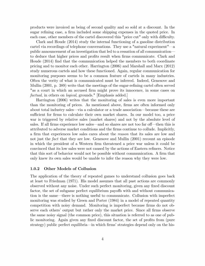
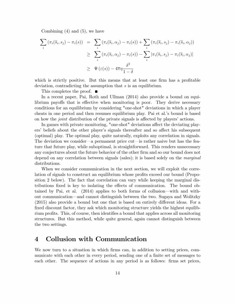
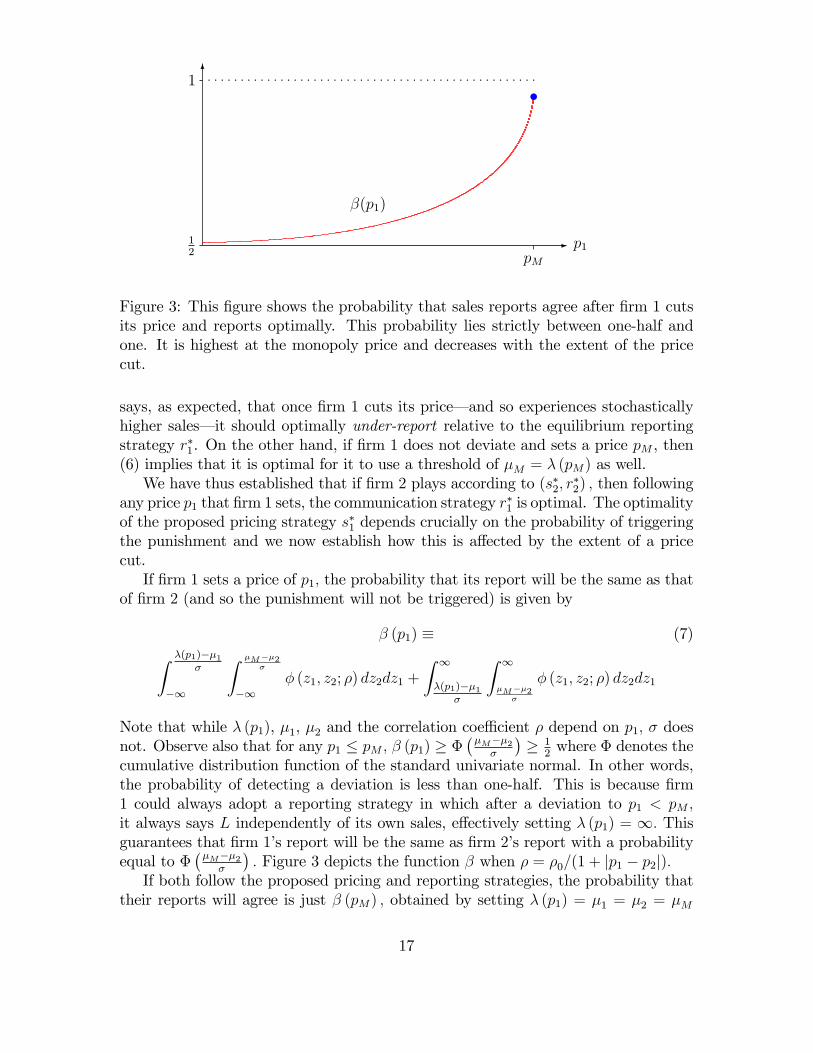
Figure 3: This figure shows the probability that sales reports agree after firm 1 cutsits price and reports optimally. This probability lies strictly between one-half andone. It is highest at the monopoly price and decreases with the extent of the pricecut.

says, as expected, that once firm 1 cuts its price– and so experiences stochasticallyhigher sales– it should optimally under-report relative to the equilibrium reportingstrategy r∗1. On the other hand, if firm 1 does not deviate and sets a price pM , then(6) implies that it is optimal for it to use a threshold of µM = λ (pM) as well.We have thus established that if firm 2 plays according to (s∗2, r

∗2) , then following

any price p1 that firm 1 sets, the communication strategy r∗1 is optimal. The optimalityof the proposed pricing strategy s∗1 depends crucially on the probability of triggeringthe punishment and we now establish how this is affected by the extent of a pricecut.If firm 1 sets a price of p1, the probability that its report will be the same as that

of firm 2 (and so the punishment will not be triggered) is given by

β (p1) ≡ (7)∫ λ(p1)−µ1σ

−∞

∫ µM−µ2σ

−∞φ (z1, z2; ρ) dz2dz1 +

∫ ∞λ(p1)−µ1

σ

∫ ∞µM−µ2

σ

φ (z1, z2; ρ) dz2dz1

Note that while λ (p1), µ1, µ2 and the correlation coeffi cient ρ depend on p1, σ doesnot. Observe also that for any p1 ≤ pM , β (p1) ≥ Φ

(µM−µ2σ

)≥ 1

2where Φ denotes the

cumulative distribution function of the standard univariate normal. In other words,the probability of detecting a deviation is less than one-half. This is because firm1 could always adopt a reporting strategy in which after a deviation to p1 < pM ,it always says L independently of its own sales, effectively setting λ (p1) = ∞. Thisguarantees that firm 1’s report will be the same as firm 2’s report with a probabilityequal to Φ

(µM−µ2σ

). Figure 3 depicts the function β when ρ = ρ0/(1 + |p1 − p2|).

If both follow the proposed pricing and reporting strategies, the probability thattheir reports will agree is just β (pM) , obtained by setting λ (p1) = µ1 = µ2 = µM

17

and ρ = ρ0 in (7). Sheppard’s formula for the cumulative of a bivariate normal (seeTihansky, 1972) implies that

β (pM) =1

πarccos (−ρ0) (8)

which is increasing in ρ0 and converges to 1 as ρ0 goes to 1. Importantly, this proba-bility does not depend on σ.

4.3 Optimality of Pricing Strategy

We have argued above that given that the other firm follows the prescribed strategy,the reporting strategy r∗1 is an optimal response for firm 1. To show that the strategies(s∗, r∗) constitute an equilibrium, it only remains to show that the pricing strategys∗1 is optimal as well. This is verified next.

Proposition 2 There exists a δ such that for all δ > δ, once σ and ρ0 are largeenough, then (s∗, r∗) constitutes an equilibrium of Gcom

δ (f) , the repeated game withcommunication.

Proof. First, note that the lifetime average profit π∗ resulting from the proposedstrategies is given by

(1− δ) πM + δ [β (pM) π∗ + (1− β (pM)) πN ] = π∗ (9)

Next, suppose that in all previous periods, both firms have followed the proposedstrategies and their reports have agreed. If firm 1 deviates to p1 < pM in the currentperiod, it gains

∆1 (p1) = (1− δ) π1 (p1, pM) + δ [β (p1) π∗ + (1− β (p1))πN ]− π∗ (10)

where π∗ is defined in (9). Thus,

∆′1 (p1) = (1− δ) ∂π1

∂p1

(p1, pM) + δβ′ (p1) [π∗ − πN ]

We will show that when σ is large enough, for all p1, ∆′1 (p1) > 0. Since ∆1 (pM) = 0,this will establish that a deviation to a price p1 < pM is not profitable. Now observethat from Lemma A.6,

limσ→∞

∆′1(p1) = (1− δ)∂π1∂p1

(p1, pM) + δ 1

π√

1−ρ20γ(p1,pM )2ρ0

∂γ∂p1

(p1, pM)× [π∗ − πN ]

≥ (1− δ) ∂π1∂p1

(pM , pM) + δ 1

π√

1−ρ20γ(0,pM )2ρ0

∂γ∂p1

(0, pM)× [π∗ − πN ]

where the last inequality uses the fact that since π1 is concave in p1,∂π1∂p1

(p1, pM) >∂π1∂p1

(pM , pM) and the fact that γ (p1, pM) is increasing and convex in p1. Let σ (δ) besuch that for all σ > σ (δ) , the inequality above holds.

18

Let δ be the solution to

(1− δ) ∂π1∂p1

(pM , pM) + δ 1

π√

1−γ(0,pM )2∂γ∂p1

(0, pM)× [π∗ − πN ] = 0 (11)

which is just the right-hand side of the inequality above when ρ0 = 1. Such a δ existssince ∂π1

∂p1(pM , pM) is finite and, by assumption, ∂ρ

∂p1(0, pM) is strictly positive. Notice

that for any δ > δ, the expression on the left-hand side is strictly positive.Now observe that

1

π√

1−ρ20γ(1,pM )2ρ0

∂γ∂p1

(0, pM)× [π∗ − πN ]

is increasing and continuous in ρ0 (recall that π∗ is increasing in ρ0). Thus, given any

δ > δ, there exists a ρ0 (δ) such that for all ρ0 = ρ0 (δ)

(1− δ) ∂π1∂p1

(pM , pM) + δ 1

π√

1−ρ20γ(0,pM )2ρ0

∂γ∂p1

(0, pM)× [π∗ − πN ] = 0

Note that ρ0 (δ) is a decreasing function of δ and for any ρ0 > ρ0 (δ) , the left-handside is strictly positive.A deviation by firm 1 to a price p1 > pM is clearly unprofitable.This completes the proof of Proposition 2.Aoyagi (2002) was the first to use threshold reporting strategies in a correlated

environment. He shows that for a given monitoring structure (ρ0 and σ fixed) as thediscount factor δ goes to one, such strategies constitute an equilibrium. The idea–as in all "folk theorems"– is that even when the probability of detection is low, ifplayers are patient enough, future punishments are a suffi cient deterrent. In contrast,Proposition 2 shows that for a given discount factor (δ high but fixed), as ρ0 goesto one and σ goes to infinity, there is an equilibrium with high profits. Its logic,however, is different from that underlying the "folk theorems" with communication,as for instance, in the work of Compte (1998) and Kandori and Matsushima (1998).In these papers, signals are conditionally independent and, in equilibrium, playersare indifferent among the messages they send. Kandori and Matsushima (1998) alsoshow that with correlation, strict incentives for "truth-telling" can be provided asis also true in our construction. But the key difference between our work and thesepapers is that in Proposition 2 the punishment power derives not from the patienceof the players; rather it comes from the noisiness of the monitoring. A deviating firmfinds it very diffi cult to predict its rival’s sales and hence, even it "lies" optimally, adeviation is very likely to trigger a punishment.The equilibrium constructed in Proposition 2 relies on using the correlation of

signals to "check" firms’reports. This is reminiscent of the logic underlying the full-surplus extraction results of Crémer and McLean (1988) but, of course, in our settingthere is no mechanism designer who can commit to arbitrarily large punishments toinduce truth-telling.

19

In our model, firms communicate simultaneously– neither firm knows the other’sreport prior to its own– and this feature is crucial to the equilibrium construction. Itis the uncertainty about what the other firm will say that disciplines firms’behavior.Often trade associations help cartels exchange sales data in a manner that is mimickedby the simultaneous reporting in our equilibrium. Cartel members make confidentialsales reports to the association which, as mentioned above, disseminates aggregatesales data to the cartel. Individual sales figures are not shared.17 Their confidentialityis usually preserved by third parties. The pocket calculator ploy mentioned in theintroduction also serves the same purpose.Finally, the "grim trigger" strategies specified above are unforgiving in that a

single disagreement at the communication stage triggers a permanent reversion tothe one-shot Nash equilibrium. Since disagreement occurs with positive probabilityeven if neither firm cheats, this means that in the long-run, collusion inevitablybreaks down. Real-world cartels do punish transgressors but these punishments arenot permanent. The equilibrium strategies we have used can easily be amended sothat the punishment phase is not permanent and that, after a pre-specified numberof periods, say T , firms return to monopoly pricing. Specifically, this means that theequilibrium profits π∗∗ are now defined by

(1− δ) πM + δ[β (pM) π∗∗ + (1− β (pM))

((1− δT+1

)πN + δT+1π∗∗

)]= π∗∗

instead of (9). For any δ > δ (as defined by (11)), there exists a T large enough sothat the forgiving strategy constitutes an equilibrium as well. Note that π∗∗ > π∗.

5 Gains from Communication

Proposition 1 shows that the profits from any equilibrium without communicationcannot exceed

2πM −Ψ−1(

4πη δ2

1−δ

)whereas Proposition 2 provides conditions under which there is an equilibrium withcommunication that with profits 2π∗ (as defined in (9)). From (8) it follows that asρ0 → 1, β (pM) → 1. Now from (9) it follows that as ρ0 → 1, π∗ → πM . Combiningthese facts leads to the formal version of the result stated in the introduction. Let δbe determined as in (11).

Theorem 1 For any δ > δ, there exist (σ (δ) , ρ0 (δ)) such that for all (σ, ρ0) �(σ (δ) , ρ0 (δ)) there is an equilibrium with communication with total profits 2π∗ suchthat

2π∗ > 2πM −Ψ−1(

4πη δ2

1−δ

)17The sharing of aggregate data is not illegal (see the discussion of the Maple Flooring case in

Areeda and Kaplow, 1988).

20

-

2πM

2π∗

2πM −Ψ−1(0)

ρ0

6

σ(δ) σ

No communication

Communicationt

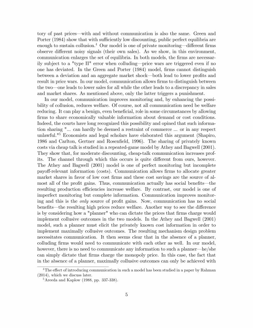
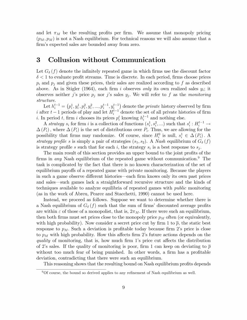
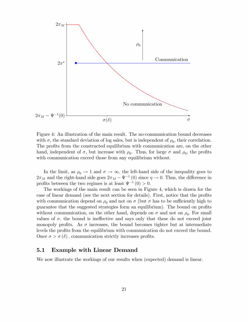
Figure 4: An illustration of the main result. The no-communication bound decreaseswith σ, the standard deviation of log sales, but is independent of ρ0, their correlation.The profits from the constructed equilibrium with communication are, on the otherhand, independent of σ, but increase with ρ0. Thus, for large σ and ρ0, the profitswith communication exceed those from any equilibrium without.

In the limit, as ρ0 → 1 and σ → ∞, the left-hand side of the inequality goes to2πM and the right-hand side goes 2πM −Ψ−1 (0) since η → 0. Thus, the difference inprofits between the two regimes is at least Ψ−1 (0) > 0.The workings of the main result can be seen in Figure 4, which is drawn for the

case of linear demand (see the next section for details). First, notice that the profitswith communication depend on ρ0 and not on σ (but σ has to be suffi ciently high toguarantee that the suggested strategies form an equilibrium). The bound on profitswithout communication, on the other hand, depends on σ and not on ρ0. For smallvalues of σ, the bound is ineffective and says only that these do not exceed jointmonopoly profits. As σ increases, the bound becomes tighter but at intermediatelevels the profits from the equilibrium with communication do not exceed the bound.Once σ > σ (δ) , communication strictly increases profits.

5.1 Example with Linear Demand

We now illustrate the workings of our results when (expected) demand is linear.

21

Suppose that18

Qi (pi, pj) = max (A− bpi + pj, 1)

where A > 0 and b > 1. For this specification, the monopoly price pM = A/2 (b− 1)and monopoly profits πM = A2/4 (b− 1) . There is a unique Nash equilibrium ofthe one-shot game with prices pN = A/ (2b− 1) and profits πN = A2b/ (2b− 1)2 .A firm’s best response if the other firm charges the monopoly price pM is to chargep = A (2b− 1) /4b (b− 1) . The highest possible profit that firm 1 can achieve whencharging a price of p is π = π1 (p, pM) = A2 (2b− 1)2 /16b (b− 1)2 .It remains to specify how the correlation between the firms’log sales is affected

by prices. In this example we adopt the following specification:

ρ =ρ0

1 + |p1 − p2|

which, of course, satisfies the assumption made in Section I.Then, recalling (1), it may be verified that for ε ∈ [0, πM/2b

2]

Ψ (ε) = ε+ A8b(b−1)2

(A− 2

√2 (b− 1) (2b− 1)

√ε)

which is achieved at equal prices. Note that Ψ (0) = πM/2b (b− 1) and Ψ−1 (0) =πM/2b

2.Finally, from (2)

η = 2Φ(

∆µmax2σ

)− 1

where ∆µmax = lnQ2 (0, pM)− lnQ2 (pM , 0) .As a numerical example, suppose A = 120 and b = 2. Let δ = 0.7 and ρ0 = 0.95.

For these parameters, πM = 3600, π = 4050 and ∆µmax = 5.19. Also, the profits fromthe equilibrium with communication, π∗ = 3524 (approximately).Figure 4 depicts the bound on profits without communication as a function of

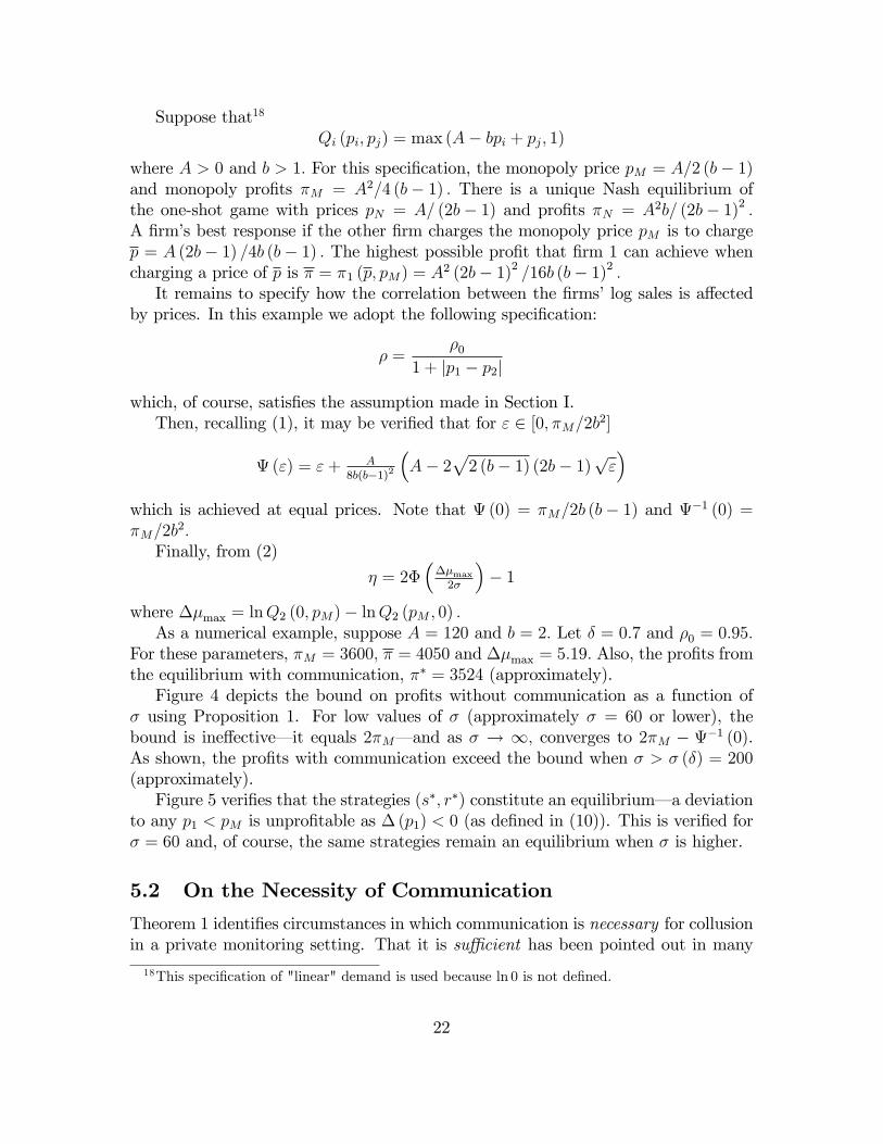
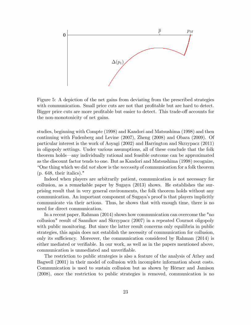
σ using Proposition 1. For low values of σ (approximately σ = 60 or lower), thebound is ineffective– it equals 2πM– and as σ → ∞, converges to 2πM − Ψ−1 (0).As shown, the profits with communication exceed the bound when σ > σ (δ) = 200(approximately).Figure 5 verifies that the strategies (s∗, r∗) constitute an equilibrium– a deviation

to any p1 < pM is unprofitable as ∆ (p1) < 0 (as defined in (10)). This is verified forσ = 60 and, of course, the same strategies remain an equilibrium when σ is higher.

5.2 On the Necessity of Communication

Theorem 1 identifies circumstances in which communication is necessary for collusionin a private monitoring setting. That it is suffi cient has been pointed out in many

18This specification of "linear" demand is used because ln 0 is not defined.

22

0pMp

0

∆(p1)

Figure 5: A depiction of the net gains from deviating from the prescribed strategieswith communication. Small price cuts are not that profitable but are hard to detect.Bigger price cuts are more profitable but easier to detect. This trade-off accounts forthe non-monotonicity of net gains.

studies, beginning with Compte (1998) and Kandori and Matsushima (1998) and thencontinuing with Fudenberg and Levine (2007), Zheng (2008) and Obara (2009). Ofparticular interest is the work of Aoyagi (2002) and Harrington and Skrzypacz (2011)in oligopoly settings. Under various assumptions, all of these conclude that the folktheorem holds– any individually rational and feasible outcome can be approximatedas the discount factor tends to one. But as Kandori and Matsushima (1998) recognize,“One thing which we did not show is the necessity of communication for a folk theorem(p. 648, their italics)."Indeed when players are arbitrarily patient, communication is not necessary for

collusion, as a remarkable paper by Sugaya (2013) shows. He establishes the sur-prising result that in very general environments, the folk theorem holds without anycommunication. An important component of Sugaya’s proof is that players implicitlycommunicate via their actions. Thus, he shows that with enough time, there is noneed for direct communication.In a recent paper, Rahman (2014) shows how communication can overcome the "no

collusion" result of Sannikov and Skrzypacz (2007) in a repeated Cournot oligopolywith public monitoring. But since the latter result concerns only equilibria in publicstrategies, this again does not establish the necessity of communication for collusion,only its suffi ciency. Moreover, the communication considered by Rahman (2014) iseither mediated or verifiable. In our work, as well as in the papers mentioned above,communication is unmediated and unverifiable.The restriction to public strategies is also a feature of the analysis of Athey and

Bagwell (2001) in their model of collusion with incomplete information about costs.Communication is used to sustain collusion but as shown by Hörner and Jamison(2008), once the restriction to public strategies is removed, communication is no

23

longer necessary for collusion.Escobar and Toikka (2013) generalize the Athey-Bagwell model to study general

repeated games with incomplete, possibly persistent, information with communica-tion. They show that with low discounting, effi cient outcomes can be approximated.On the other hand, Escobar and Llanes (2015) derive conditions under which ef-ficiency cannot be attained without communication. The two results then isolatecircumstances in which, for low discounting, communication is necessary to achieveeffi ciency.In a different vein, Awaya (2014a) studies the prisoners’dilemma with private

monitoring and shows that for a fixed discount rate, there exist environments in whichwithout communication, the only equilibrium is the one-shot equilibrium whereaswith communication, almost perfect cooperation can be sustained. This paper is aprecursor to the current one.Finally, the necessity of communication has been studied in laboratory experi-

ments as well (by Fonseca and Normann (2012) and Cooper and Kühn (2014) amongothers). These experiments, however, do not involve imperfect monitoring and so donot directly address the issues dealt with in this paper.

6 Conclusion

We have provided theoretical support for the idea that even unverifiable commu-nication within a cartel facilitates greater collusion and is detrimental for society.How does "cheap talk" aid collusion? When the monitoring is poor, and there isno communication, a price cut cannot be detected with any confidence and this isthe basis of the bound developed in Proposition 1. With communication, however,the probability that a price cut will trigger a punishment is significant relative tothe short-term gains. Thus, communication reduces the type II error associated withimperfect monitoring and this is the driving force behind our main result.It has been argued (Carlton et al., 1996) that the exchange of information among

firms is beneficial to society because it improves the allocation of resources. Considera firm that experiences high sales. If it learns, in addition, that other firms havealso experienced high sales, then it would rightly infer that its own high sales are theresult of a market-wide positive demand shock. If this is likely to persist in the future,a firm can then increase production and investment with greater confidence. In thispaper, however, demand shocks are independent across periods. Last period’s salesthus carry information about the rival’s past behavior but reveal nothing about futuredemand. Thus, any positive effect resulting from information exchange is absent. Amodel in which demand shocks are persistent would incorporate both effects and,perhaps, be able to measure the trade-off. This remains a project for future research.We emphasize that in this paper, we have not explored the role of communication

in coordinating cartel behavior– agreeing on prices, market shares and transfers,among other things. Since cartels cannot sign binding contracts enforced by third

24

parties, presumably they can only coordinate on strategies that form an equilibrium.Pre-play communication would then serve to select one among many equilibria (seeGreen, Marshall and Marx, 2014). But a theory of how communication helps firmsselect among equilibria, while important for antitrust practice, remains a challenge.

A Appendix

A.1 Collusion without Communication

A.1.1 Non-responsive Strategies

The ex ante distribution over Pj in period t induced by a strategy profile s is

αtj (s) = Es[stj(h

t−1j )] ∈ ∆ (Pj) (12)

Given a strategy profile s, recall that αj denotes the strategy of firm i in which itplays αtj (s) in period t following any t− 1 period history. The strategy αj replicatesthe ex ante distribution of prices resulting from s but is non-responsive to histories.The following lemma shows that the function Ψ, defined in (1), which determines

the incentives versus effi ciency trade-off in the one-shot game, embodies the sametrade-off in a repeated setting if the non-deviating player follows a non-responsivestrategy. It shows that to minimize the average incentive to deviate while achievingaverage profits within ε of 2πM one should split the incentive evenly across periods.The lemma resembles an intertemporal "consumption smoothing" argument (recallthat Ψ is convex).

Lemma A.1 (Smoothing) For any strategy profile s whose profits exceed 2πM − ε,∑i

[πi (si, αj (s))− πi (s)] ≥ Ψ (ε)

where si denotes firm i’s strategy in which it sets p following any history.

Proof. Define

ε (t) = 2πM − Es[∑

i

πi(st(ht−1))

]as the difference between the sum of monopoly profits 2πM and the sum of expectedprofits in period t. Now clearly (1− δ)

∑∞t=1 δ

tε (t) ≤ ε.

25

Then, ∑i

[πi (si, αj (s))− πi (s)]

= Es

[(1− δ)

∞∑t=1

δt∑i

[πi(p, ptj

)− πi

(pti, p

tj

)]]≥ (1− δ)

∞∑t=1

δtΨ (ε (t))

≥ Ψ

((1− δ)

∞∑t=1

δtε (t)

)≥ Ψ (ε)

The first equality follows from the fact that the induced distribution over prices ptjis the same under (si, αj) as it is under s. The second inequality follows from thedefinition of Ψ. The third and fourth result from the fact that Ψ is convex andnon-increasing, respectively.

A.1.2 Weak Monitoring

For a fixed strategy pair (s1, s2), let λtj be the induced probability distribution over

firm j’s private histories htj ∈ H tj = (Pj × Yj)t ⊂ R2t. Similarly, let λ

t

j be the proba-bility distribution over j’s private histories induced by the strategy pair (si, sj).

19 Wewish to determine the total variation distance between λtj and λ

t

j.The total variation distance between two distributions G and G over Rn is equal

to ∥∥G−G∥∥TV

= 12

sup‖ϕ‖∞≤1

∣∣E [ϕ]− E [ϕ]∣∣ (13)

where E and E denote the expectations with respect to the distributions G andG, respectively and the supremum is taken over all measurable functions ϕ with supnorm ‖ϕ‖∞ ≤ 1. Note that the definition in (13) is equivalent to the one in Definition1. See, for instance, Levin, Peres and Wilmer (2009).As a first step, we decompose the total variation distance between two probabil-

ity distributions into the distance between their marginals and that between theirconditionals.

Lemma A.2 Given two distributions G and G over Rm × Rn,∥∥G−G∥∥TV≤∥∥GX −GX

∥∥TV

+ supx

∥∥GY |X −GY |X∥∥TV

where GX is the marginal distribution of G on Rm and GY |X (· | x) is the conditionaldistribution of G on Rn given X = x (and similarly for G).

19Recall that si denotes the strategy of firm i in which it sets p with probability one following anyhistory.

26

Proof. Let E and E denote the expectations with respect to G and G, respectively.Given any function ϕ : Rm × Rn → [−1, 1] , we have

12

∣∣E [ϕ]− E [ϕ]∣∣ = 1

2

∣∣EX [EY |X [ϕ]]− EX

[EY |X [ϕ]

]∣∣≤ 1

2

∣∣EX [EY |X [ϕ]]− EX

[EY |X [ϕ]

]∣∣+1

2

∣∣EX

[EY |X [ϕ]

]− EX

[EY |X [ϕ]

]∣∣≤ 1

2sup‖ϕ‖∞≤1

∣∣EX [ϕ]− EX [ϕ]∣∣+ 1

2EX

[∣∣EY |X [ϕ]− EY |X [ϕ]∣∣]

≤∥∥GX −GX

∥∥TV

+ EX

[∥∥GY |X −GY |X∥∥TV

]≤

∥∥GX −GX

∥∥TV

+ supx

∥∥GY |X −GY |X∥∥TV

and so ∥∥G−G∥∥TV

= 12

sup‖ϕ‖∞≤1

∣∣E [ϕ]− E [ϕ]∣∣

≤∥∥GX −GX

∥∥TV

+ supx

∥∥GY |X −GY |X∥∥TV

which is the required inequality.Next we show that given a history ht−1

j , the total variation distance between thetwo conditional distributions cannot exceed the monitoring quality.

Lemma A.3 For any ht−1j ,∥∥∥λtj(· | ht−1

j )− λtj(· | ht−1j )∥∥∥TV≤ η

Proof. Let Sj(· | ht−1j ) denote the distribution of prices that j’s strategy sj induces

after j’s private history ht−1j . Similarly, let Si(· | ht−1

i ) denote the distribution of prices

that i’s strategy induces after i’s private history ht−1i . Let Si(· | ht−1

j ) = E[Si(· |ht−1i ) | ht−1

j ] denote j’s expectation about i’s distribution of prices, given j’s own

history ht−1j . Finally, let S(p | ht−1

j ) = Si(pi | ht−1j )Sj(pj | ht−1

j ) denote the jointdistribution of prices that j expects given j’s private history ht−1

j (recall that firms’choices are independent).

27

Now, for any ϕ : Pj × Yj → [−1, 1]

I(ϕ) ≡∣∣∣∣∣∫Pj×Yj

ϕdλtj(· | ht−1j )−

∫Pj×Yj

ϕdλt

j(· | ht−1j )

∣∣∣∣∣=

∣∣∣∣∣∫Pi

∫Pj

∫Yj

ϕdFj (yj | p) dSj(pj | ht−1j )dSi(pi | ht−1

j )

−∫Pj

∫Yj

ϕdFj (yj | p, pj) dSj(pj | ht−1j )

∣∣∣∣∣=

∣∣∣∣∣∫P

∫Yj

ϕdFj (yj | p) dS(p | ht−1j )−

∫P

∫Yj

ϕdFj (yj | p, pj) dS(p | ht−1j )

∣∣∣∣∣where the second equality follows by integrating∫

Pj

∫Yj

ϕdFj (yj | p, pj) dSj(pj | ht−1j )

over pi using the distribution Si(· | ht−1j ). Thus,

I(ϕ) =

∣∣∣∣∣∫P

∫Yj

ϕ [fj (yj | p)− fj (yj | p, pj)] dyjdS(p | ht−1j )

∣∣∣∣∣≤

∫P

[∫Yj

|ϕfj (yj | p)− ϕfj (yj | p, pj)| dyj

]dS(p | ht−1

j )

≤ 2

∫P

ηdS(p | ht−1j )

= 2η

where the second inequality follows from the definition of total variation.Thus, ∥∥∥λtj(· | ht−1

j )− λtj(· | ht−1j )∥∥∥TV

= 12

sup‖ϕ‖∞≤1

I(ϕ)

≤ η

as was to be shown.Combining the preceding two lemmas we obtain the key result that the total

variation distance between λtj and λt

j is bounded above by a linear function of time.

Lemma A.4 For all t, ∥∥∥λtj − λtj∥∥∥TV≤ tη

28

Proof. The proof is by induction. For t = 1, there is no history and Lemma A.3implies the result directly.Now suppose that the result holds for t− 1. Using Lemma A.2, we have∥∥∥λtj − λtj∥∥∥

TV≤

∥∥∥λt−1j − λt−1

j

∥∥∥TV

+ supht−1j

∥∥∥λtj(· | ht−1j )− λtj(· | ht−1

j )∥∥∥TV

≤ (t− 1) η + η

by the induction hypothesis and Lemma A.3.The next result verifies the intuition that when the monitoring quality is low, the

profits of a deviator who undertakes a permanent price cut are not too different fromthose when its rival follows a distributionally equivalent non-responsive strategy. Theimportance of the lemma is in quantifying this difference.

Lemma A.5 Let α be the non-responsive strategy as defined in (12). Then,

|πi (si, sj)− πi (si, αj)| ≤ 2πηδ2

1− δ

where π = maxpj πi (p, pj) .

Proof. As above, let λtj be the distribution over firm j’s private histories htj induced

by (si, sj) and let λt

j be the distribution over j’s private histories induced by (si, sj) .Then,

πi (si, sj) = (1− δ)∞∑t=1

δt∫Ht−1j

E[πi (p, sj) | ht−1j ]dλj(h

t−1j )

Also, if Sj(· | ht−1j ) denotes the distribution over j’s prices induced by the strategy

sj following the history ht−1j , then

πi (si, αj) = (1− δ)∞∑t=1

δt∫Pj

πi (p, pj) dαtj (pj)

= (1− δ)∞∑t=1

δt∫Pj

πi (p, pj)

(∫Ht−1j

dSj(pj | ht−1j )dλj(h

t−1j )

)

= (1− δ)∞∑t=1

δt∫Ht−1j

E[πi (p, sj) | ht−1j ]dλj(h

t−1j )

since by definition

αtj (pj) =

∫Ht−1j

Sj(pj | ht−1j )dλj(h

t−1j )

29

Thus,

|πi (si, sj)− πi (si, αj)|

≤ (1− δ)∞∑t=1

δt

∣∣∣∣∣∫Ht−1j

E[πi (p, sj) | ht−1j ](dλj(h

t−1j )− dλj(ht−1

j ))

∣∣∣∣∣≤ 2πη (1− δ)

∞∑t=1

δt (t− 1)

= 2πηδ2

1− δ

where the second inequality is a consequence of Lemma A.4 and the fact that, as in(13), given any two distributions λ and λ,

∣∣E [ϕ]− E [ϕ]∣∣ ≤ 2 ‖ϕ‖∞ ×

∥∥λ− λ∥∥TVfor

any bounded measurable function ϕ.

A.2 Collusion with Communication

Lemma A.6 For any p1 ≥ 1,

limσ→∞

β′ (p1) =1

π√

1− ρ20γ (p1, pM)2

× ρ0

∂γ

∂p1

(p1, pM)

Proof. First, we derive β′ (p1) . Since λ is optimally chosen, the envelope theoremguarantees that

∂β (p1)

∂λ= 0

and so∂β (p1)

∂µ1

= −∂β (p1)

∂λ= 0

as well.Thus, we have

β′ (p1) =∂β (p1)

∂ρ

∂ρ

∂p1

+∂β (p1)

∂µ2

∂µ2

∂p1

Now, since we can write

β (p1) = 2Φ(λ(p1)−µ1

σ, µM−µ2

σ; ρ)

+ Φ(λ(p1)−µ1

σ

)+ Φ

(µM−µ2σ

)− 1

where

Φ (z1, z2; ρ) = Pr [Z1 ≥ z1, Z2 ≥ z2] =

∫ ρ

−1

φ (z1, z2; θ) dθ

30

using Sheppard’s formula20 (see Tihansky, 1972) and Φ is the cumulative distributionfunction of a standard univariate normal. Thus,

∂β (p1)

∂ρ= 2φ

(λ(p1)−µ1

σ, µM−µ2

σ; ρ)

which converges to 2φ (0, 0; ρ) = 1/π√

1− ρ2 as σ →∞.Finally,

∂β (p1)

∂µ2

=1

σ

∫ λ−µ1σ

−∞φ(z1,

µM−µ2σ

; ρ)dz1 −

∫ ∞λ−µ1σ

φ(z1,

µM−µ2σ

; ρ)dz1

=

1

σ

[2Φ(

1−ρ2ρ

µM−µ2σ

)− 1]φ(µM−µ2

σ

)This converges to 0 as σ →∞.This completes the proof.

References

[1] Abreu, Dilip, David Pearce and Ennio Stacchetti. (1990): "Toward a Theory ofDiscounted Repeated Games with Imperfect Monitoring," Econometrica, 58 (5),1041—1063.

[2] Areeda, Philip and Louis Kaplow (1988): Antitrust Analysis: Problems, Text,Cases (4th edition), Little, Brown and Company, Boston.

[3] Aoyagi, Masaki (2002): "Collusion in Dynamic Bertrand Oligopoly with Cor-related Private Signals and Communication," Journal of Economic Theory, 102(1), 229—248.

[4] Athey, Susan and Kyle Bagwell (2001): "Optimal Collusion with Private Infor-mation," Rand Journal of Economics, 32 (3), 428—465

[5] Awaya, Yu (2014a): "Private Monitoring and Communication in Re-peated Prisoners’ Dilemma," Working Paper, Penn State University,http://www.personal.psu.edu/yxa120/research.html

[6] Awaya, Yu (2014b): "Cooperation without Monitoring," Working Paper, PennState University, http://www.personal.psu.edu/yxa120/research.html

[7] Carlton, Dennis W., Robert H. Gertner, Andrew M. Rosenfield (1996): "Com-munication among Competitors: Game Theory and Antitrust," George MasonLaw Review, 5, 423—440.

20This employs a change of variables to the original formula.

31

[8] Clark, Robert and Jean-François Houde (2014): "The Effect of Explicit Commu-nication on Pricing: Evidence from the Collapse of a Gasoline Cartel," Journalof Industrial Economics, 62 (2), 191—227.

[9] Compte, Olivier (1998): "Communication in Repeated Games with ImperfectPrivate Monitoring," Econometrica, 66 (3), 597—626.

[10] Cooper, David and Kai-Uwe Kühn (2014): "Communication, Renegotiation, andthe Scope for Collusion," American Economic Journal: Microeconomics, 6 (2):247—278.

[11] Crémer, Jacques, and Richard P. McLean (1988): "Full Extraction of the Surplusin Bayesian and Dominant Strategy Auctions," Econometrica, 56 (6): 1247—1257.

[12] Escobar, Juan and Llanes, Gastón (2015): "Cooperation Dynamics in RepeatedGames of Adverse Selection," Working Paper, University of Chile.

[13] Escobar, Juan F. and Juuso Toikka (2013): "Effi ciency in Games with MarkovianPrivate Information," Econometrica, 81 (5): 1887—1934.

[14] Fonseca, Miguel A. and Hans-Theo Normann (2012): "Explicit vs. TacitCollusion– The Impact of Communication in Oligopoly Experiments," EuropeanEconomic Review, 56 (8), 1759—1772.

[15] Friedman, James (1971): "A Non-cooperative Equilibrium for Supergames," Re-view of Economic Studies, 38 (1), 1—12.

[16] Fudenberg, Drew and David K. Levine (2007): "The Nash-Threats Folk Theo-rem with Communication and Approximate Common Knowledge in Two PlayerGames," Journal of Economic Theory, 132 (1), 461—473.

[17] Genesove, David and Wallace P. Mullin (2001): "Rules, Communication, andCollusion: Narrative Evidence from the Sugar Institute Case," American Eco-nomic Review, 91 (3), 379—398.

[18] Green, Edward J., Robert C. Marshall and Leslie Marx: "Tacit Collusion inOligopoly," in Roger D. Blair and D. Daniel Sokol (eds.), Oxford Handbook ofInternational Antitrust Economics, Volume 2, Oxford: Oxford University Press,2014, pp. 464—497.

[19] Green, Edward J. and Robert Porter (1984): "Noncooperative Collusion underImperfect Price Information," Econometrica, 52 (1), 87—100.

[20] Harrington, Joseph E. (2006): "How do Cartels Operate?" Foundations andTrends in Microeconomics, 2 (1), 1-105.

32

[21] Harrington, Joseph E. and Andrzej Skrzypacz (2011): "Private Monitoring andCommunication in Cartels: Explaining Recent Collusive Practices," AmericanEconomic Review, 101 (6), 2425—2449.

[22] Hörner, Johannes and Julian Jamison (2007): "Collusion with (Almost) no In-formation," The RAND Journal of Economics, 38 (3), 804—822.

[23] Kandori, Michihiro and Hitoshi Matsushima (1998): "Private Observation, Com-munication and Collusion," Econometrica, 66 (3), 627—652.

[24] Levin, David A., Yuval Peres and Elizabeth L. Wilmer (2009): Markov Chainsand Mixing Times, Providence: American Mathematical Society.

[25] Mailath, George and Larry Samuelson (2006): Repeated Games and Reputations,Oxford: Oxford University Press.

[26] Marshall, Robert C. and Leslie Marx (2012): The Economics of Collusion, Cam-bridge: MIT Press.

[27] Obara, Ichiro (2009): "Folk Theorem with Communication," Journal of Eco-nomic Theory, 144 (1), 120—134.

[28] Pai, Mallesh, Aaron Roth and Jonathan Ullman (2014): "An Anti-Folk Theorem for Large Repeated Games with Imperfect Monitoring,"http://arxiv.org/abs/1402.2801v2 [cs.GT]

[29] Sannikov, Yuliy and Andrzej Skrzypacz (2007): “Impossibility of Collusion underImperfect Monitoring with Flexible Production,”American Economic Review,97 (5): 1794—1823.

[30] Shapiro, Carl (1986): "Exchange of Cost Information in Oligopoly," Review ofEconomic Studies, 53 (3), 433—446.

[31] Stigler, George (1964): "A Theory of Oligopoly," Journal of Political Economy,74 (1), 44—61.

[32] Sugaya, Takuo (2013): "Folk Theorem in Repeated Gameswith Private Monitoring," Working Paper, Stanford University,https://sites.google.com/site/takuosugaya/home/research

[33] Sugaya, Takuo and Alexander Wolitzky (2015): "On the EquilibriumPayoff Set in Repeated Games with Imperfect Private Monitoring,"http://economics.mit.edu/faculty/wolitzky/research

[34] Tihansky, Dennis P. (1972): "Properties of the Bivariate Normal CumulativeDistribution," Journal of the American Statistical Association, 67 (340), 903—905.

33

[35] Zheng, Bingyong (2008): "Approximate Effi ciency in Repeated Games with Cor-related Private Signals," Games and Economic Behavior, 63 (1), 406—416.

34