On Coupling of Discrete Random Walks on the Line

Örn Arnaldsson

30 ECTS thesis submitted in partial fulfillment of aMagister Scientiarum degree in Mathematics

AdvisorHermann Þórisson

Faculty of Natural SciencesSchool of Engineering and Physical Sciences

University of IcelandReykjavik, May 2010

On Coupling of Discrete Random Walks on the Line30 ECTS thesis submitted in partial fulfillment of a Magister Scientiarum degree inMathematics

Copyright c© 2010 Örn ArnaldssonAll rights reserved

Faculty of Physical SciencesSchool of Engineering and Natural SciencesUniversity of IcelandVRII, Hjarðarhagi 2-6107 ReykjavíkIceland

Telephone: 525 4000

Bibliographic information:Örn Arnaldsson, 2010, On Coupling of Discrete Random Walks on the Line, Master’sthesis, Faculty of Physical Sciences, University of Iceland.

Printing: HáskólafjölritunReykjavík, Iceland, May 2010

Abstract

The main focus of this thesis is on coupling of random walks on the line with discretestep lengths and initial positions. After introducing the relevant coupling concepts,an Ornstein-type approach is used to establish necessary and sufficient conditions forthe existence of a successful exact coupling and a successful shift-coupling. This yieldsresults on asymptotic loss of memory. These findings are then applied to establishsuccessful exact coupling of continuous-time regenerative processes with discrete re-generation times. After preliminaries on extension techniques, we finally construct asuccessful exact coupling of random walks with non-discrete (possibly singular) steplengths that are periodic in a certain sense.

iii

Contents

Acknowledgements v

Notation vii

1 Introduction 1

2 Coupling Concepts 2

3 Exact Coupling – Fixed Initial Positions 4

4 Exact Coupling – Random Initial Positions 9

5 Shift-Coupling 13

6 Classical Regeneration 16

7 Transfer and Splitting 22

8 Non-Discrete Step-Lengths 27

References 30

iv

Acknowledgements

First, I would like to thank Professor Hermann Þórisson for all his kind help during mystudies at the University of Iceland and his good ideas regarding this project. I wouldalso like to thank the Dux Squad; my fellow student and friend Einar Bjarki Gunnarssonfor his help with LATEX and my friend Magnús Sigurðsson for all the commas. TomWaits I thank for keeping me company during the typing. Finally, I want to thank mygirlfriend Ásta for all her love.

v

a

Swing, pretty girl, swing.It ain’t real anyway.

David Lynch, Imaginary Girl

vi

Notation

• All random walks in this paper are on the line, R. We shall simply call themrandom walks.

• If f is a measurable function from the measurable space (E, E) into the measur-able space (G,G), we say that f is E/G-measurable.

• If A is a countable set, the σ-algebra of all its subsets will be denoted by 2A.

• If A is a topological space, we will denote the Borel σ-algebra on A by B(A).

• R∞ will denote the set (x0, x1, x2, . . .) : xi ∈ R, i ≥ 0.

• If X is a random element with distribution µ, we will write X ∼ µ. If two randomelements X and Y have the same distribution, we write X D

= Y and we say thatY is a copy of X.

• If P is a probability measure, we say that something holds P -a.s. (P -almostsurely) if it holds on a set of P -measure 1. We will simply say that somethingholds almost surely if it is clear which probability measure is being referred to.

• Similarly, if (Ω,F , P ) is a probability space, we say that something holds forP -a.e. (P -almost every) ω in A ∈ F , if it holds on a subset of A having massP (A).

• If µ is a probability measure and A is a set such that µ(A) = 1, we will writeµ ∈ A.

vii

1 Introduction

A random walk on the line is a sequence S = (Sn)n≥0 of random variables whereSn = S0 +X1 +X2 + . . .+Xn for some independent random variables S0, X1, X2, . . ..The walk, S, is a random element in (R∞,B(R∞)). We call S0 the initial positionof S and X1, X2, . . . are called the step-lengths of S. If S0 ∼ λ and X1, X2, . . . arei.i.d. having distribution µ we say that S is a (λ, µ) random walk. If S0 is concentratedon a constant s a.s., we say that S is an (s, µ) random walk. Most of the random walkswe will discuss have discrete step-length and initial distributions (a.s. take their valuesin some countable set). We say these are discrete.

The main question we will deal with is the following: If S is a (λ, µ) random walkand S is a (λ′, µ) random walk, does there exist a successful exact coupling of S andS ′? That is, do there exist random elements (S, S ′, T ), defined on the same probabilityspace (Ω,F , P ), such that T is a P -a.s. finite random time on N (coupling time), S D

= S,S ′

D= S ′, and θT S = θT S

′, where

θn : R∞ → R∞, θn((x0, x1, . . .)) = (xn, xn+1, . . .),

with the convention that θT S = θT S′ on the null-set T = ∞? In other words, S is

a (λ, µ) random walk, S ′ is a (λ′, µ) random walk and S and S ′ are exactly the samefrom the time T onwards.

Note that sinceh : (N,R∞)→ R∞, h(n, s) = θn(s)

is 2N ⊗ (B(R))∞/(B(R))∞-measurable and

(θT S)(ω) = θT (ω)S(ω)

is a composition of ω 7→ (T (ω), S(ω)) and h, θTS is a random element, that is, θTS isF/(B(R))∞-measurable.

A successful shift-coupling of S and S ′ are random elements (S, S ′, T, T ′) such thatS

D= S, S ′ D= S ′ and θT S = θT ′S

′, where T and T ′ are P -a.s. finite random times. Thatis, S and S ′ do visit the same real number (though it may happen at different times)and they are exactly the same from those times onward.

A successful coupling allows us to establish, via the coupling event inequality,asymptotic loss of memory of the random walks; two random walks with differentinitial distributions but the same step-length distribution will behave in the same wayin the end. This method dates back to a 1938 paper by Doeblin [1] where his classi-cal coupling established an irreducible, positive recurrent Markov chain’s convergence

1

to equilibrium. In the random walk case, there is no equilibrium possible since therecurrent random walks on R are null-recurrent.

In 1969, Ornstein [2] constructed a successful exact coupling of (possibly transient)(λ, µ) and (λ′, µ) random walks S and S ′, respectively, on a lattice dZ, d > 0, when theset A = a ∈ R : P (X1 = a) > 0 is strongly aperiodic: A set A ⊆ dZ, d > 0, where dis such that A is in no strict sub-lattice of dZ (A is aperiodic in dZ), is called stronglyaperiodic if there is an a ∈ A such that A− a is not contained in any strict sub-latticeof dZ.

Section 2 contains preliminaries on coupling. In Section 3, we use a similar trick asOrnstein to couple discrete random walks that need not be in a lattice. We will alsosee that Ornstein’s condition of strong aperiodicity of the step-lengths is a special caseof a more general theorem about discrete random walks. A theorem that gives a nec-essary and sufficient condition on A = a ∈ R : P (X1 = a) > 0 for a successful exactcoupling of random walks in the additive subgroup generated by A to always exist. InSection 4, we will show that a successful shift-coupling of discrete random walks onthis group always exists. From our results on discrete random walks, we can deduceresults for random walks whose step-length distributions (that need not be identical)have a discrete component. In Section 5, we apply these shift-coupling results to estab-lish results on exact coupling for certain continuous-time regenerative processes. Afterpreliminaries on extension techniques in Section 6, we finally, in Section 7, construct asuccessful exact coupling for random walks with singular-continuous step-length com-ponents that are periodic in a certain sense. This is modeled after Thorisson’s [3]treatment of random walks with spread-out step-lengths (these are step-lengths suchthat the sum of several of them has a non-singular distribution). As an example wewill look at a random walk with a step-length distribution on the “double” Cantor-set,C ∪ (C − 1).

2 Coupling Concepts

This section is based on Chapter 1, Sections 4 and 5, of [3].

Definition 2.1. A coupling of a collection of random elements Yi, i ∈ I, is a familyof random elements (Yi)i∈I, all defined on some probability space (Ω,F , P ), such thatYi

D= Yi for all i ∈ I.

Definition 2.2. Let (Yi)i∈I be a coupling of Yi, i ∈ I. An event C is called a coupling

2

event of the coupling (Yi)i∈I if

Yi = Yj on C for all i, j ∈ I.

Another concept important to us is the following.

Definition 2.3. For a bounded, signed measure ν in some measurable space (E, E),we define its total variation norm as

‖ν‖ := supA∈E

ν(A)− infA∈E

ν(A).

It is easy to see that ‖ · ‖ defines a norm on the vector space of all bounded, signedmeasures on (E, E). We obtain the following proposition on the total variation normof the difference of two probability measures.

Proposition 2.4. Let P and Q be probability measures on some measurable space(E, E), then we have

‖P −Q‖ = 2 supA∈E

(P (A)−Q(A)) = 2 supA∈E|P (A)−Q(A)|.

Proof. Since A ∈ E if and only if Ac ∈ E and since for any set B ⊆ R, inf (−B) =

− sup (B), we get

‖P −Q‖ = supA∈E

(P (A)−Q(A))− infA∈E

(P (A)−Q(A))

= supA∈E

(P (A)−Q(A)) + supA∈E

(Q(A)− P (A))

= supA∈E

(P (A)−Q(A)) + supAc∈E

(Q(Ac)− P (Ac))

= supA∈E

(P (A)−Q(A)) + supAc∈E

(1−Q(A)− (1− P (A)))

= supA∈E

(P (A)−Q(A)) + supAc∈E

(P (A)−Q(A)))

= 2 supA∈E

(P (A)−Q(A)).

And since ‖P −Q‖ = ‖Q− P‖ (‖ · ‖ being a norm) we obtain

‖P −Q‖ = 2 supA∈E

(P (A)−Q(A)) = 2 supA∈E

(Q(A)− P (A)) = 2 supA∈E|P (A)−Q(A)|.

Thus, convergence of probability measures in the total variation norm is strongerthan weak convergence. Next, we establish the coupling event inequality of a couplingof two random elements.

3

Theorem 2.5. Let (Y , Y ′) be a coupling of two random elements, Y and Y ′ in (E, E),with coupling event C. Then

‖P (Y ∈ ·)− P (Y ′ ∈ ·)‖ ≤ 2P (Cc) (Coupling Event Inequality).

Proof. Since Y = Y ′ on C we get, for A ∈ E ,

P (Y ∈ A,C) = P (Y ′ ∈ A,C),

and thus

P (Y ∈ A)− P (Y ′ ∈ A) = P (Y ∈ A)− P (Y ′ ∈ A)

= P (Y ∈ A,Cc)− P (Y ∈ A,Cc)

≤ P (Cc).

Thus

‖P (Y ∈ ·)− P (Y ′ ∈ ·)‖ = 2 supA∈E

(P (Y ∈ A)− P (Y ′ ∈ A))

≤ 2P (Cc).

Therefore, the greater the total variation difference of P (Y ∈ ·) and P (Y ′ ∈ ·) is,the smaller the probability of a coupling event will be. This means we can not find acoupling (Y , Y ′), of Y and Y ′, with a coupling event of high probability if the originalY and Y ′ do not have similar distributions, that is if ‖P (Y ∈ ·)− P (Y ′ ∈ ·)‖ is large.

Having defined coupling and the important concepts related to it, we turn to randomwalks.

3 Exact Coupling – Fixed Initial Positions

In this section we shall use an Ornstein-type approach to couple discrete (s, µ) and(s′, µ) random walks. Ornstein’s method of finding a successful exact coupling of twodifferently started random walks, S and S ′, on a lattice was, in short, as follows. Let Sand S ′ be independent and construct a third random walk S ′′, such that the differencewalk S − S ′′ is sure to hit zero at an a.s. finite random time T . Then define S ′′′ to bethe process following S ′′ until time the T and then switching to S. The walk S ′′′ turnsout to be a copy of S ′ and hence (S, S ′′′, T ) is a successful exact coupling of S and S ′.

We need one preliminary result on simple symmetric random walks on a lattice dZ,d > 0, that is, a random walk with initial distribution on the lattice, with i.i.d. step-length distribution ν, such that ν(−d, 0, d) = 1 and ν(d) = ν(−d) > 0. The result is

4

well known and is often proved using Stirling’s formula: for large n, n! ∼√

2πn(n/e)n.We give the more elementary hitting probability proof (Gambler’s ruin).

Lemma 3.1. A simple, symmetric random walk R on the lattice dZ, d > 0, hits zerowith probability one.

Proof. We prove the assertion for d = 1, the proof for general d > 0 is analogous. Letν be the step-length distribution of R. Put qi = P (R never hits 0 | R0 = i), i ∈ Z.Then q0 = 0 and qi = q−i. For i ≥ 1, we get qi = ν(−1)qi−1 + ν(1)qi+1 + ν(0)qi. Thus,qi+1 − qi = qi − qi−1 = . . . = q1 − q0 = q1 and we get

qi =i∑

k=1

(qk − qk−1) =i∑

k=1

q1 = iq1.

Therefore, q1 = 0 and it follows that qi = 0 for all i ∈ Z.

The first theorem gives a necessary and sufficient condition for the existence of asuccessful exact coupling when λ and λ′ are concentrated on some constants s and s′,respectively. But first we set up some terminology and establish a lemma.

Define, for a distribution µ on R, the set

Aµ := a ∈ R : µ(a) > 0.

Let B ⊆ R. Define a(B) to be the smallest additive group containing B, that is

a(B) = n1b1 + · · ·+ nkbk : k ∈ N, n1, . . . , nk ∈ Z and b1, . . . , bk ∈ B.

Let B −B be the set bi − bj : bi, bj ∈ B. Note that a(B −B) ⊆ a(B) for any B ⊆ Rand if B is countable, then a(B) is also countable. Further, if B is non-lattice. that is,B 6⊆ dZ for all d > 0, then a(B) is dense in R (see [3], page 61, for a proof).

Lemma 3.2. Let B ⊆ R be countable. Then B ⊆ a(B − B) if and only if a(B) =

a(B −B).

Proof. If a(B) = a(B − B), then obviously B ⊆ a(B − B). If on the other handB ⊆ a(B − B), then, since a(B) is the smallest additive group containing B, it mustbe contained in a(B−B). But since a(B−B) ⊆ a(B), we have a(B) = a(B−B).

We will adopt the following convention throughout the paper: If X is a discreterandom element, defined on some probability space (Ω,F , P ), taking values in somecountable set A a.s., we shall assume thatX(ω) ∈ A for all ω ∈ Ω. This is no restrictionsince we can define X on any null-set as we wish without changing its distribution.

5

Therefore, in the following, when X1, X2, . . . are the step-lengths of some discrete (λ, µ)

random walk, we will assume that for each i ≥ 1 and ω ∈ Ω, Xi(ω) ∈ Aµ.We come now to our key result.

Theorem 3.3. Let S and S ′ be discrete (s, µ) and (s′, µ) random walks, respectively.There exists a successful exact coupling, (S, S ′, T ), of S and S ′ if and only if s− s′ ∈a(Aµ − Aµ).

Proof. Let (S, S ′, T ) be a successful exact coupling of S and S ′, defined on some prob-ability space (Ω,F , P ), and let X1, X2, . . . be the step-lengths of S and X ′1, X ′2, . . . thestep-lengths of S ′. Then there is an ω ∈ Ω such that T (ω) < ∞. Since ST = S ′T , weget

s+ X1(ω) + X2(ω) + . . .+ XT (ω)(ω) = s′ + X ′1(ω) + X ′2(ω) + . . .+ X ′T (ω)(ω)

which is equivalent to

s− s′ = (X1(ω)− X ′1(ω)) + (X2(ω)− X ′2(ω)) + . . .+ (XT (ω)(ω)− X ′T (ω)(ω)).

The right hand side is in a(Aµ − Aµ) and the only if part follows.Now assume d := s− s′ ∈ a(Aµ −Aµ). It is no restriction to assume that S and S ′

are independent, defined on some probability space (Ω,F , P ). Call the step-lengths ofS and S ′, X1, X2, . . . and X ′1, X ′2, . . ., respectively. We break the rest of the proof intofour steps.

Step 1: There is an r ∈ N such that

P (X1 +X2 + . . .+Xr − (X ′1 +X ′2 + . . .+X ′r) = d) > 0.

Since d ∈ a(Aµ−Aµ), we can write, for some r ≥ 0 and a1, a2, . . . , ar, a′1, a′2, . . . , a

′r ∈ Aµ,

d = (a1 − a′1) + (a2 − a′2) + . . .+ (ar − a′r).

Then

P (X1 +X2 + . . .+Xr − (X ′1 +X ′2 + . . .+X ′r) = d)

≥ P (X1 = a1, X2 = a2, . . . , Xr = ar, X′1 = a′1, X

′2 = a′2, . . . , X

′r = a′r).

Since all the Xi, X′i are independent and µ(a) > 0 for all a ∈ Aµ, this is strictly greater

than zero.

6

Step 2: Construction of a third random walk S ′′.

For k ≥ 1, let

Yk := (X(k−1)r+1, X(k−1)r+2, . . . , Xkr),

and Y ′k := (X ′(k−1)r+1, X′(k−1)r+2, . . . , X

′kr).

Obviously, (Y1, Y′

1), (Y2, Y′

2), . . . is an i.i.d. sequence of random elements in R2r, andsince Yk and Y ′k are independent and have the same distribution, we also have (Yk, Y

′k)

D=

(Y ′k , Yk).Define, for k ≥ 1,

Lk := X(k−1)r+1 +X(k−1)r+2 + . . .+Xkr

and L′k := X ′(k−1)r+1 +X ′(k−1)r+2 + . . .+X ′kr.

Notice that (Lk, L′k) is a measurable function of (Yk, Y

′k) and since (Yk, Y

′k)

D= (Y ′k , Yk),

we get

P (Yk ∈ ·, |Lk − L′k| = d) = P (Y ′k ∈ ·, |L′k − Lk| = d). (∗)

We now construct the step-lengths of a third random walk. Notice that by Step 1,P (|Lk − L′k| = d) = P (Lk − L′k = d) + P (L′k − Lk = d) > 0. Let

(X ′′(k−1)r+1, . . . , X′′kr) :=

Yk if |Lk − L′k| 6= d,

Y ′k if |Lk − L′k| = d.

Since Y ′′k := (X ′′(k−1)r+1, . . . , X′′kr) is the same measurable function of (Yk, Y

′k) for each

k ≥ 1, the Y ′′k are i.i.d. Further, for C ∈ B(Rr) and k ≥ 1, we get

P (Y ′′k ∈ C) = P (Y ′′k ∈ C, |Lk − L′k| 6= d) + P (Y ′′k ∈ C, |Lk − L′k| = d)

= P (Yk ∈ C, |Lk − L′k| 6= d) + P (Y ′k ∈ C, |Lk − L′k| = d)

= P (Yk ∈ C, |Lk − L′k| 6= d) + P (Yk ∈ C, |Lk − L′k| = d)

= P (Yk ∈ C),

where the third equality follows by (∗). Thus, X ′′1 , X ′′2 , . . . are i.i.d. with distribution µand if we define a random walk S ′′ with initial position s′ and step-lengths X ′′1 , X ′′2 , . . .,it is a (s′, µ) random walk. We also have

L′′k := X ′′(k−1)r+1 +X ′′(k−1)r+2 + . . .+X ′′kr =

Lk if |Lk − L′k| 6= d,

L′k if |Lk − L′k| = d.

7

Step 3: S and S ′′ meet.

Let R = (Rk)k≥0 be the difference walk of S and S ′′, with step-lengths (Xk −X ′′k )k≥1,beginning in s − s′ = d. Now, let us observe R only at times 0, r, 2r, 3r, . . .. Thestep-lengths of (Rkr)k≥0 are Lk − L′′k and, remembering the definition of L′′k, we get

Lk − L′′k =

0 if |Lk − L′k| 6= d,

d if Lk − L′k = d,

−d if L′k − Lk = d.

By Step 1, the random walk (Rkr)k≥0 is a simple symmetric random walk on the latticedZ. By Lemma 3.1, (Rkr)k≥0 will hit zero at an a.s. finite random time K, so

0 = RKr = SKr − S ′′Kr.

Thus, S and S ′′ meet at the a.s. finite random time T := Kr.

Step 4: Construction of a successful exact coupling.

Define the discrete-time stochastic process S ′′′ = (s′ +X ′′′1 + . . .+X ′′′n )n≥0, where

X ′′′k =

X ′′k if k ≤ T,

Xk if k > T.

That is, S ′′′ follows S ′′ until it meets S and then it switches to S.The random elements (S, S ′′′, T ) give us a successful exact coupling of S and S ′

if we can establish that S ′′′ is indeed a (s′, µ) random walk. It suffices to show thatthe step-lengths X ′′′1 , X

′′′2 , . . . are i.i.d. with distribution µ, and to that end it suffices

to prove that Y ′′′1 , Y′′′

2 , . . . are i.i.d. having the same distribution as Y1 (where Y ′′′k :=

(X ′′′(k−1)r+1, . . . , X′′′kr)): For n ≥ 1 and A1, A2, . . . , An ∈ B(Rr), we have (remember that

T = Kr)

P (Y ′′′1 ∈ A1, . . . , Y′′′n ∈ An)

=∞∑i=1

P (Y ′′′1 ∈ A1, . . . , Y′′′n ∈ An, K = i)

=n−1∑i=1

P (Y ′′1 ∈ A1, . . . , Y′′i ∈ Ai, K = i, Yi+1 ∈ Ai+1, . . . , Yn ∈ An)

+∞∑i=n

P (Y ′′1 ∈ A1, . . . , Y′′n ∈ An, K = i).

8

The event K = i is determined by (Y1, Y2, . . . , Yi) and (Y ′1 , Y′

2 , . . . , Y′i ) and is

therefore independent of both (Yi+1, Yi+2, . . .) and (Y ′i+1, Y′i+2, . . .). By Step 2, Y ′′1 , Y ′′2 , . . .

are i.i.d. with the same distribution as Y1. Since Y ′′i+1, Y′′i+2, . . . are determined by

(Yi+1, Yi+2, . . .) and (Y ′i+1, Y′i+2, . . .), the random elements Y ′′i+1, Y

′′i+2, . . . are also inde-

pendent of K = i. Now, continuing the calculations above:

P (Y ′′′1 ∈ A1, . . . , Y′′′n ∈ An)

=n−1∑i=1

P (Y ′′1 ∈ A1, . . . , Y′′i ∈ Ai, K = i)P (Yi+1 ∈ Ai+1, . . . , Yn ∈ An)

+∞∑i=n

P (Y ′′1 ∈ A1, . . . , Y′′n ∈ An, K = i)

=n−1∑i=1

P (Y ′′1 ∈ A1, . . . , Y′′i ∈ Ai, K = i)P (Y ′′i+1 ∈ Ai+1, . . . , Y

′′n ∈ An)

+∞∑i=n

P (Y ′′1 ∈ A1, . . . , Y′′n ∈ An, K = i)

=n−1∑i=1

P (Y ′′1 ∈ A1, . . . , Y′′n ∈ An, K = i)

+∞∑i=n

P (Y ′′1 ∈ A1, . . . , Y′′n ∈ An, K = i)

=∞∑i=1

P (Y ′′1 ∈ A1, . . . , Y′′n ∈ An, K = i)

= P (Y ′′1 ∈ A1, . . . , Y′′n ∈ An)

= P (Y ′′1 ∈ A1)P (Y ′′2 ∈ A2) · · · P (Y ′′n ∈ An).

Thus, Y ′′′1 , Y′′′

2 , . . . are i.i.d. having the same distribution as Y1 and therefore S ′′′ is a(s′, µ) random walk.

Example 3.4. Let µ have a uniform distribution on the set √

2, π, e, 42. Let Sand S ′ be (

√2, µ) and (π, µ) random walks, respectively. By Theorem 3.3, there exist

copies, S and S ′, of S and S ′, respectively, such that S and S ′ are the same from ana.s. finite random time onward.

4 Exact Coupling – Random Initial Positions

A random walk is a sequence of partial sums of random variables. Due to this additivenature it is natural to observe random walks in some additive sub-group of R. If arandom walk has step-lengths in some lattice dZ, d > 0, it is natural to restrict the

9

possible initial distributions to the same lattice to be sure that the walk is in dZ. Ifa random walk has step-lengths with continuous distributions, we observe it on thewhole line R, allowing any initial distribution.

Therefore, if a random walk has some general discrete step-length distribution µ, itis natural to restrict the possible initial distribution to the additive sub-group generatedby Aµ. This is the aforementioned a(Aµ). In this natural setting we establish a theoremgiving a necessary and sufficient condition on Aµ for there always to exist a successfulexact coupling of two random walks.

Theorem 4.1. Let S and S ′ be discrete (λ, µ) and (λ′, µ) random walks, respectively.The following are equivalent.

(i) There exists a successful exact coupling, (S, S ′, T ), of S and S ′, for all λ, λ′ ∈a(Aµ).

(ii) a(Aµ) = a(Aµ − Aµ).

Proof. (i) ⇒ (ii): Let d ∈ a(Aµ) and choose λ and λ′ to be concentrated at d and 0,respectively. Let (S, S ′, T ) be a successful exact coupling of S and S ′, defined on someprobability space (Ω,F , P ), and let X1, X2, . . . be the step-lengths of S and X ′1, X ′2, . . .the step-lengths of S ′. Then there is an ω ∈ Ω such that T (ω) <∞, and since

ST (ω)(ω) = S ′T (ω)(ω),

we getd+ X1(ω) + . . .+ XT (ω)(ω) = 0 + X ′1(ω) + . . .+ X ′T (ω)(ω),

and isolating d gives

d = (X1(ω)− X ′1(ω)) + . . .+ (XT (ω)(ω)− X ′T (ω)(ω)).

The right hand side is in a(Aµ − Aµ), thus a(Aµ) ⊆ a(Aµ − Aµ). Since the reverseinclusion always holds, we have a(Aµ) = a(Aµ − Aµ).

(ii)⇒ (i): Now assume a(Aµ) = a(Aµ−Aµ). Let S and S ′ be (λ, µ) and (λ′, µ) randomwalks, respectively, where λ and λ′ are probability distributions on a(Aµ).

Let S0 and S ′0 be independent a(Aµ)-valued random variables with distributionsλ and λ′, respectively, defined on some probability space (Ω,F , P ). On the sameprobability space let there be defined, independent of (S0, S

′0), a countable collection

of independent random elements

(S(s,s′), S′(s,s′), T(s,s′)), s, s′ ∈ a(Aµ) = a(Aµ − Aµ),

10

where for each pair (s, s′), with s, s′ ∈ a(Aµ),

(S(s,s′), S′(s,s′), T(s,s′))

is a successful exact coupling of a (s, µ) and a (s′, µ) random walk. Because s − s′ ∈a(Aµ) = a(Aµ − Aµ), we know these random elements exist by Theorem 3.3.

We define our candidate for a successful exact coupling of S and S ′ as

(S, S ′, T ) := (S(S0,S′0), S′(S0,S′0)

, T(S0,S′0)).

To see that P (S ∈ C) = P (S(S0,S′0) ∈ C) = P (S ∈ C), for C ∈ B(R∞), note that

P (S(S0,S′0) ∈ C) =∑

s′∈a(Aµ)

∑s∈a(Aµ)

P (S(S0,S′0) ∈ C, S0 = s, S ′0 = s′)

=∑

s′∈a(Aµ)

∑s∈a(Aµ)

P (S(s,s′) ∈ C, S0 = s, S ′0 = s′)

=∑

s′∈a(Aµ)

∑s∈a(Aµ)

P (S(s,s′) ∈ C)P (S0 = s)P (S ′0 = s′)

=∑

s′∈a(Aµ)

( ∑s∈a(Aµ)

P (S(s,s′) ∈ C)λ(s)

)λ′(s′)

=∑

s′∈a(Aµ)

P (S ∈ C)λ′(s′)

= P (S ∈ C).

Therefore S is indeed a (λ, µ) random walk and similarly we get that S ′ is a (λ′, µ)

random walk. Finally, observe that for P -a.e. ω in S0 = s, S ′0 = s′ we have

(θT S)(ω) = θT (ω)S(S0(ω),S′0(ω))(ω) = θT(s,s′)(ω)S(s,s′)(ω)

= (θT(s,s′)S(s,s′))(ω) = (θT(s,s′)S′(s,s′))(ω)

= (θT S ′)(ω).

Since⋃s,s′∈a(Aµ)S0 = s, S ′0 = s′ is a countable partition of the probability space, T is

a.s. finite andθT S = θT S ′.

Example 4.2. Let µ be a distribution on the rational numbers, Q, such that µ(q) > 0

for all q ∈ Q. Let λ and λ′ be some distributions on Q and let S and S ′ be (λ, µ) and(λ′, µ) random walks, respectively. Since obviously a(Q) = a(Q−Q), by Theorem 4.1,there exist copies, S and S ′, of S and S ′, respectively, such that S and S ′ are the samefrom an a.s. finite random time onward.

11

According to the following Proposition, Theorem 4.1 is a direct extension of Orn-stein’s result.

Proposition 4.3. Let A ⊆ R be contained in some lattice dZ, d > 0, such thatA is not contained in a strict sub-lattice of dZ (i.e. A is aperiodic in dZ). Then thefollowing are equivalent.

(i) a(A) = a(A− A).

(ii) A is strongly aperiodic.

Proof. (i)⇒ (ii): If A is not strongly aperiodic, then A−a is in some strict sub-latticeof dZ for all a ∈ A. This means that a(A−A) is in some strict sub-lattice of dZ. Butsince A itself is in no such sub-lattice, we get A * a(A− A). Thus a(A) 6= a(A− A),by Lemma 3.2.

(ii)⇒ (i): If A is strongly aperiodic, there is some a ∈ A such that A− a is aperiodicin dZ. This means that dZ = a(A − a) ⊆ a(A − A), since aperiodic sets in dZspan the whole lattice. Thus A ⊆ a(A − A) which, by Lemma 3.2, is equivalent toa(A) = a(A− A).

Although the condition a(A) = a(A−A) is equivalent to strong aperiodicity whenA is in a lattice, it is not clear if the condition has any simpler or “deeper” meaningwhen A is non-lattice, that is A 6⊆ dZ for all d > 0. One thing we can say though is thatif Aµ is the set a1, a2, . . . and a1, a2, . . . are linearly independent over the integers,then a(Aµ) 6= a(Aµ−Aµ). To see this, define the mapping ϕ : a(Aµ)→ Z/2Z such thatϕ(ai) = 1, for all ai ∈ Aµ. Then, since ϕ(a′) = 0 for all a′ ∈ a(Aµ − Aµ), a(Aµ − Aµ)

can not be the same set as a(Aµ).Theorems 3.3 and 4.1 yield asymptotic results for discrete random walks.

Corollary 4.4. Let S and S ′ be random walks with a discrete step-length distributionµ. Let s, s′ ∈ R be such that s − s′ ∈ a(Aµ − Aµ) and let λ and λ′ be probabilitydistributions on a(Aµ). Suppose that either one of the following conditions is satisfied:

(a) S0 = s a.s. and S ′0 = s′ a.s.

(b) S0 ∼ λ, S ′0 ∼ λ′ and a(Aµ) = a(Aµ − Aµ).

Then we get asymptotic loss of memory of S and S ′, that is

‖P (Sn ∈ ·)− P (S ′n ∈ ·)‖ → 0, as n→∞.

12

Proof. If S0 = s a.s. and S ′0 = s′ a.s., by Theorem 3.3, there exists a successful exactcoupling, (S, S ′, T ), of S and S ′. Then T ≤ n is a coupling event of the coupling(Sn, S

′n) of Sn and S ′n. By the coupling event inequality, we have

‖P (Sn ∈ ·)− P (S ′n ∈ ·)‖ ≤ 2P (T > n),

and since T is a.s. finite, we get

‖P (Sn ∈ ·)− P (S ′n ∈ ·)‖ → 0, as n→∞.

Theorem 4.1 gives the same result when S0 ∼ λ, S ′0 ∼ λ′ and a(Aµ) = a(Aµ −Aµ).

The method of proof in Theorem 3.3 works for a larger class of random walks thandiscrete with i.i.d. step-lengths: LetH andH ′ be two differently started, not necessarilydiscrete random walks. Assume H and H ′ are independent and let H0 = s a.s. andH ′0 = s′ a.s. Let d = s− s′ and let X1, X2, . . . and X ′1, X ′2, . . . be the step-lengths of Hand H ′, respectively, where

X1 ∼ µ1, X2 ∼ µ2, . . . , X′1 ∼ µ1, X

′2 ∼ µ2, . . . ,

for some sequence µ1, µ2, . . . of distributions. If there is an r such that infk≥1 P (Lk −L′k = d) > 0, where Lk := X(k−1)r+1 + . . .+Xkr and L′k := X ′(k−1)r+1 + . . .+X ′kr, thenthe same proof as in Theorem 3.3 will work to find a successful exact coupling of Hand H ′.

The theorems of this section can be used to establish some similar results on theexistence of a successful shift-coupling of two differently started, discrete random walks.This will be our next topic.

5 Shift-Coupling

We begin by proving an analog of Theorem 3.3 for shift-coupling.

Theorem 5.1. Let S and S ′ be discrete (s, µ) and (s′, µ) random walks, respectively.There exists a successful shift-coupling, (S, S ′, T, T ′), of S and S ′ if and only if s− s′ ∈a(Aµ).

Proof. Let (S, S ′, T, T ′) be a successful shift-coupling of S and S ′, on some probabilityspace (Ω,F , P ). Then there is an ω ∈ Ω such that T (ω) <∞, and since

ST (ω)(ω) = S ′T ′(ω)(ω),

13

we gets+ X1(ω) + . . .+ XT (ω)(ω) = s′ + X ′1(ω) + . . .+ X ′T ′(ω)(ω),

which is equivalent to

s− s′ = X1(ω) + . . .+ XT (ω)(ω)− (X ′1(ω) + . . .+ X ′T ′(ω)(ω)).

The right hand side is in a(Aµ), proving the only if part.For the if part, let d := s− s′ ∈ a(Aµ). If 0 ∈ Aµ then a(Aµ) = a(Aµ−Aµ) and the

result follows by Theorem 3.3. Suppose that 0 6∈ Aµ and define A0µ := Aµ∪0. Define

a distribution ν on A0µ by requiring that ν(0) = 1/2 and ν(a | Aµ) = µ(a) for a ∈ Aµ.

Let R and R′ be (s, ν) and (s′, ν) random walks, respectively. Since 0 ∈ Aν = A0µ, we

get a(Aν) = a(Aν − Aν) and according to Theorem 4.1, there exists a successful exactcoupling, (R, R′, K), of R and R′. Call the step-lengths of R and R′, Y1, Y2, . . . andY1

′, Y2

′, . . ., respectively. Observe the random walks that emerge if we only look at R

and R′ when their step-lengths are not zero; define

τ0 := 0 and, recursively, τi+1 := minn > τi : Yn 6= 0,

and define τ ′i in a similar way from Y ′1 , Y′

2 , . . .. Now, define the stochastic processesS := (s + Yτ1 + . . . + Yτn)n≥0 and S ′ := (s′ + Y ′τ ′1

+ . . . + Y ′τ ′n)n≥0. Since Yτ1 , Yτ2 . . . areindependent, having distribution µ, S is a (s, µ) random walk. Similarly, S ′ is a (s′, µ)

random walk. Define

O := #n ≥ 1 : Yn = 0, n ≤ K and O′ := #n ≥ 1 : Y ′n = 0, n ≤ K.

That is, O is the number of zero jumps of R before the coupling time K and O′ is thenumber of zero jumps of R′ before K. Since (R, R′, K) is a successful exact couplingof R and R′, R and R′ are exactly the same from the time K onwards. Thus S and S ′

are exactly the same from the times T := K − O and T ′ := K − O′, respectively, and(S, S ′, T, T ′) is a successful shift-coupling of S and S ′.

Next, we establish the existence of a successful shift-coupling of discrete randomwalks in the natural setting.

Theorem 5.2. Let S and S ′ be discrete (λ, µ) and (λ′, µ) random walks whereλ, λ′ ∈ a(Aµ). Then there exists a successful shift-coupling, (S, S ′, T, T ′), of S and S ′.

Proof. Let S0 and S ′0 be independent with distributions λ and λ′, respectively. Defineon the same probability space, independent of S0 and S ′0, the independent quadruples

(S(s,s′), S′(s,s′), T(s,s′), T

′(s,s′)), s, s′ ∈ a(Aµ),

14

where (S(s,s′), S′(s,s′), T(s,s′), T

′(s,s′)) is a successful shift-coupling of a (s, µ) and a (s′, µ)

random walk as in Theorem 5.1. Define

(S, S ′, T, T ′) := (S(S0,S′0), S′(S0,S′0)

, T(S0,S′0), T′(S0,S′0)

).

By similar calculations as in the proof of Theorem 4.1, we get that (S, S ′, T, T ′) is asuccessful shift-coupling of S and S ′.

We obtain asymptotic results on discrete random walks as a corollary to the abovetheorems.

Corollary 5.3. Let S and S ′ be random walks with a discrete step-length distributionµ. Let s, s′ ∈ R be such that s−s′ ∈ a(Aµ) and let λ and λ′ be probability distributionson a(Aµ). Suppose that either one of the following conditions is satisfied:

(a) S0 = s a.s. and S ′0 = s′ a.s.

(b) S0 ∼ λ and S ′0 ∼ λ′.

Then we get Cesaro (time-average) total variation convergence of S and S ′, that is,

‖ 1

n

n−1∑k=0

P (Sk ∈ ·)−1

n

n−1∑k=0

P (S ′k ∈ ·)‖ → 0, as n→∞.

Proof. By theorems 5.1 and 5.2, if either one of the conditions (a) or (b) are satisfied,there exists a successful shift-coupling, (S, S ′, T, T ′), of S and S ′. By Proposition 2.4,we get

‖ 1

n

n−1∑k=0

P (Sk ∈ ·)−1

n

n−1∑k=0

P (S ′k ∈ ·)‖ = 2 supA∈B(R)

| 1n

n−1∑k=0

P (Sk ∈ A)− 1

n

n−1∑k=0

P (S ′k ∈ A)|

= 2 supA∈B(R)

| 1n

n−1∑k=0

P (Sk ∈ A)− 1

n

n−1∑k=0

P (S ′k ∈ A)|

= 2 supA∈B(R)

|E[1

n

n−1∑k=0

1Sk∈A −1

n

n−1∑k=0

1S′k∈A]|.

Now, we can write

|E[n∑k=0

1Sk∈A −n∑k=0

1S′k∈A]|

= |E[1T<T ′(n∑k=0

1Sk∈A −n∑k=0

1S′k∈A) + 1T≥T ′(

n∑k=0

1Sk∈A −n∑k=0

1S′k∈A)]|,

15

and since ST+k = S ′T ′+k, for k ≥ 0, we get, with the convention that∑n

k=n xk = 0,

|E[1T<T ′(n∑k=0

1Sk∈A −n∑k=0

1S′k∈A)]|

= |E[1T<T ′(T∧n−1∑k=0

1Sk∈A +n∑

k=T∧n

1Sk∈A −T ′∧n−1∑k=0

1S′k∈A−

n∑k=T ′∧n

1S′k∈A)]|

= |E[1T<T ′(T∧n−1∑k=0

1Sk∈A +n∑

k=T∧n+(n−T ′∧n)

1Sk∈A −T ′∧n−1∑k=0

1S′k∈A)]|

≤ E[1T<T ′(T ∧ n+ (n− (T ∧ n+ (n− T ′ ∧ n))) + T ′ ∧ n)]

≤ 4E[1T<T ′(T′ ∧ n)].

Similarly we obtain

|E[1T≥T ′(n∑k=0

1Sk∈A −n∑k=0

1S′k∈A)]| ≤ 4E[1T≥T ′(T ∧ n)],

and thus

|E[n∑k=0

1Sk∈A −n∑k=0

1S′k∈A]|

= |E[1T<T ′(n∑k=0

1Sk∈A −n∑k=0

1S′k∈A) + 1T≥T ′(

n∑k=0

1Sk∈A −n∑k=0

1S′k∈A)]|

≤ 4E[1T<T ′(T′ ∧ n)] + 4E[1T≥T ′(T ∧ n)]

= 4E[(T ∨ T ′) ∧ n].

Finally, we get

‖ 1

n

n−1∑k=0

P (Sk ∈ ·)−1

n

n−1∑k=0

P (S ′k ∈ ·)‖ = 2 supA∈B(R)

|E[1

n

n−1∑k=0

1Sk∈A −1

n

n−1∑k=0

1S′k∈A]|

≤ 8

nE[(T ∨ T ′) ∧ (n− 1)]→ 0 as n→∞.

Where the convergence in the last step follows by a.s. finiteness of T and T ′ anddominated convergence.

6 Classical Regeneration

The following introduction to classical regeneration is based on Chapter 10, Sections 2and 3, in [3].

16

Let (Ω,F , P ) be a probability space, supporting the random elements

Z = (Zt)t∈[0,∞) and S = (Sn)n≥0,

where Z is a one-sided continuous-time stochastic process taking values in some space(E, E) and S is a sequence of random times, satisfying

0 ≤ S0 < S1 < S2 < . . .→∞.

The process Z is a random element in (G,G) := (E[0,∞), E [0,∞)), where E [0,∞) is theσ-algebra spanned by the projection mappings πt : E[0,∞) 7→ E, π(z) = zt. We regardS as an element in the sequence space (L,L), where

L := (sn)n≥0 ∈ [0,∞)N : s0 < s1 < . . .→∞

and L are the Borel subsets of L: L = L ∩ (B[0,∞))N. Thus, (Z, S) is a randomelement in (G× L,G ⊗ L).

The random times S split Z into a delay

D := (Zt)t∈[0,S0)

and cyclesCn := (ZSn−1+t)t∈[0,Xn),

where Xn are the cycle-lengths

Xn = Sn − Sn−1.

After time S0, the delay, D, is in some external state (cemetery-state) ∆ 6∈ E and Cn isin ∆ after timeXn. Thus, the delay and cycles are one-sided continuous-time stochasticprocesses taking values in the measurable space (E∆, E∆) := (E ∪ ∆, σ(E ∪ ∆)) andare random elements in (E

[0,∞)∆ , E [0,∞)

∆ ), where as before, E [0,∞)∆ is spanned by the finite

dimensional projections. Let θt, where t ≥ 0, be the shift map from G to G,

θt(z) = (zt+s)s∈[0,∞).

Let θt also denote the joint shift map from G× L to G× L:

θt(z, s) = (θt(z), (snt+k − t)k≥0),

where nt := minn ≥ 1 : sn ≥ t. If A is any countable set in [0,∞), then the mapping(t, (z, s)) 7→ θt(z, s) is 2A ⊗ G ⊗ L/G ⊗ L-measurable. Thus, if T is a random timeon (Ω,F , P ), such that for each ω ∈ Ω we have T (ω) ∈ AT , where AT is countable

17

(we shall assume this is the case for all discrete random times in this section), thenθT (Z, S) is a random element in G × L. All the random times we will encounter inthis section will be discrete and therefore we shall have no problems when shifting bya random time.

A successful exact coupling of two one-sided continuous-time processes Z and Z ′ arerandom elements (Z, Z ′, T ) such that T is a.s. finite, Z D

= Z, Z ′ D= Z ′ and θT Z = θT Z′.

After these preliminaries, we come to the definition of this section’s main concept.

Definition 6.1. A one-sided, continuous-time stochastic process Z is said to beclassically regenerative with regeneration times S if, for all n ≥ 0, we have

θSn(Z, S)D= θS0(Z, S).

andθSn(Z, S) is independent of ((Zs)s∈[0,Sn), S0, S1, . . . , Sn).

In other words, (Z, S) regenerates at the times S, that is it starts anew, indepen-dently of the past. The above definition can be reformulated as follows (see [3], page346 for a proof).

Proposition 6.2. Z is classically regenerative with regeneration times S if and onlyif the cycles C1, C2, C3, . . . are i.i.d. and independent of the delay D.

Notice that S is a random walk with initial position S0 and step-lengths X1, X2, . . .

when Z is classically regenerative with regeneration times S. Another pair (Z ′, S ′)

is called a version of a classically regenerative (Z, S) if (Z ′, S ′) is itself classicallyregenerative and

θS′0(Z′, S ′)

D= θS0(Z, S).

Thus, a version, (Z ′, S ′), of a classically regenerative process (Z, S) has the same cycle-distribution but the delay-distributions may differ; (Z ′, S ′) is a differently started ver-sion of (Z, S). By Proposition 6.2, if (Z, S) is classically regenerative then clearly S isa random walk with positive i.i.d. step-lengths.

An example of a classically regenerative process is the GI/GI/k queue that emptiesinfinitely often, with the successive entrance times to an empty system as regenerationtimes.

A renewal process is a (λ, µ) random walk, S, with a positive initial position S0 andstrictly positive step-lengths X1, X2 . . .. We call S0 the delay of S while the X1, X2, . . .

are called life times in the renewal context (the analogy being that the X1, X2, . . . arethe life times of light bulbs that are replaced by a new one the moment they burn out,

18

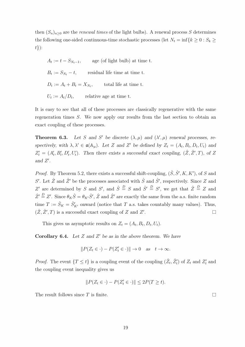
then (Sn)n≥0 are the renewal times of the light bulbs). A renewal process S determinesthe following one-sided continuous-time stochastic processes (let Nt = infk ≥ 0 : Sk ≥t):

At := t− SNt−1, age (of light bulb) at time t.

Bt := SNt − t, residual life time at time t.

Dt := At +Bt = XNt , total life at time t.

Ut := At/Dt, relative age at time t.

It is easy to see that all of these processes are classically regenerative with the sameregeneration times S. We now apply our results from the last section to obtain anexact coupling of these processes.

Theorem 6.3. Let S and S ′ be discrete (λ, µ) and (λ′, µ) renewal processes, re-spectively, with λ, λ′ ∈ a(Aµ). Let Z and Z ′ be defined by Zt = (At, Bt, Dt, Ut) andZ ′t = (A′t, B

′t, D

′t, U

′t). Then there exists a successful exact coupling, (Z, Z ′, T ), of Z

and Z ′.

Proof. By Theorem 5.2, there exists a successful shift-coupling, (S, S ′, K,K ′), of S andS ′. Let Z and Z ′ be the processes associated with S and S ′, respectively. Since Z andZ ′ are determined by S and S ′, and S

D= S and S ′

D= S ′, we get that Z D

= Z andZ ′

D= Z ′. Since θKS = θK′S

′, Z and Z ′ are exactly the same from the a.s. finite randomtime T := SK = S ′K′ onward (notice that T a.s. takes countably many values). Thus,(Z, Z ′, T ) is a successful exact coupling of Z and Z ′.

This gives us asymptotic results on Zt = (At, Bt, Dt, Ut).

Corollary 6.4. Let Z and Z ′ be as in the above theorem. We have

‖P (Zt ∈ ·)− P (Z ′t ∈ ·)‖ → 0 as t→∞.

Proof. The event T ≤ t is a coupling event of the coupling (Zt, Z′t) of Zt and Z ′t and

the coupling event inequality gives us

‖P (Zt ∈ ·)− P (Z ′t ∈ ·)‖ ≤ 2P (T ≥ t).

The result follows since T is finite.

19

Thus, At, Bt, Dt and Ut, in the end, forget how they started.

More generally, we can apply the results from the last two sections to find a suc-cessful exact coupling of two regenerative processes when the delay and cycle-lengthsare discrete.

Theorem 6.5. Let (Z, S) be classically regenerative with discrete delay-length dis-tribution λ and discrete cycle-length distribution µ. Let (Z ′, S ′) be a version of (Z, S)

with discrete delay-length distribution λ′. If λ, λ′ ∈ a(Aµ), then there exists a successfulexact coupling, (Z, Z ′, T ), of Z and Z ′.

Proof. Let D,C1, C2, . . . be the delay and cycles of (Z, S) and let D′ be the delay of(Z ′, S ′). By Proposition 6.2, C1, C2, . . . are i.i.d. and independent of D. By Theorem5.2, there exists a successful shift-coupling, (S, S ′, K,K ′), of S and S ′. Let Sn =

S0 + X1 + . . .+ Xn and S ′n = S ′0 + X ′1 + . . .+ X ′n. Define, independent of (S, S ′, K,K ′),the countable independent collection

(Cx1 , C

′x1 , C

x2 , C

′x2 , C

x3 , C

′x3 , . . .), x ∈ Aµ,

where, for each x ∈ Aµ, Cx1 , C

′x1 , C

x2 , C

′x2 , C

x3 , C

′x3 , . . . are i.i.d. and for all i ≥ 1,

P (Cxi ∈ ·) = P (C

′xi ∈ ·) = P (C1 ∈ · | X1 = x).

Independent of all of these random elements, let Dy, y ∈ a(Aµ), be a countable collec-tion of independent random elements with

P (Dy ∈ ·) = P (D ∈ · | S0 = y),

and independent of all the random elements above, let D′y, y ∈ a(Aµ), be a countablecollection of independent random elements with

P (D′y ∈ ·) = P (D′ ∈ · | S ′0 = y).

Now define the stochastic processes Z, with delay DS0 and cycles CX11 , CX2

2 , . . . and Z ′

with delay D′S′0 and cycles C′X′11 , C

′X′22 , . . ..

The cycles CX11 , CX2

2 , . . . are obviously i.i.d. and independent of DS0 . For i ≥ 1, we

20

get

P (CXii ∈ ·) =

∑x∈a(Aµ)

P (CXii ∈ ·, Xi = x)

=∑

x∈a(Aµ)

P (Cxi ∈ ·)P (Xi = x)

=∑

x∈a(Aµ)

P (Cxi ∈ ·)P (X1 = x)

=∑

x∈a(Aµ)

P (C1 ∈ ·, X1 = x)

= P (C1 ∈ ·),

where the fourth equality follows directly from the definition of Cxi . Similarly, we get:

DS0D= D, D′S′0 D

= D′ and for i ≥ 1, C′X′ii

D= C1. Thus Z and Z ′ are copies of Z and Z ′,

respectively.By definition, for i ≥ 1, the cycle CXi

i has length Xi, while the cycle CX′ii has length

X ′i. Now, since (S, S ′, K,K ′) is a successful shift-coupling of S and S ′, we have thatT := SK = S ′K′ is an a.s. finite random time at which Z and Z ′ share a regenerationtime. Define a third process Z ′′, following Z ′ until the time T , and then switching toZ. The cycles of Z ′′ are

C ′′i =

C′X′ii if i ≤ K ′

CXK+(i−K′)K+(i−K′) if i > K ′.

By a similar argument as in step 4 of the proof of Theorem 3.3, C ′′1 , C ′′2 , . . . are i.i.d. andindependent ofD′S′0 , having the same distribution as C1. Thus, (Z, Z ′′, T ) is a successfulexact coupling of Z and Z ′.

Again, we obtain a corollary on asymptotic loss of memory, the proof is the sameas in Corollary 6.4.

Corollary 6.6. Let (Z, S) and (Z ′, S ′) be as in the above theorem. We have

‖P (Zt ∈ ·)− P (Z ′t ∈ ·)‖ → 0 as t→∞.

If we could choose Z ′ to be stationary, that is Z ′ D= θtZ′ for all t ≥ 0, the above

corollary would yield that Zt converges to stationarity in total variation. However,this can not be done since a stationary version of Z has a continuous delay-lengthdistribution (while S ′0 is discrete) with density P (X1>x)

E[X1](see [3], page 65 for proof).

21

7 Transfer and Splitting

Next, we will look at random walks whose step-lengths have singular components. Sincewe are dealing with components of the step-lengths, we shall need some new conceptsand techniques before we can move on. This section is based on Chapter 3, Sections 4and 5 of [3].

We say that a probability space, (Ω, F , P ), is an extension of the probability space(Ω,F , P ) if there is a F/F -measurable mapping ξ such that P−1ξ = P , that is P (ξ ∈A) = P (A), A ∈ F . The term extension stems from the fact that every random elementon (Ω,F , P ) also exists on (Ω, F , P ), that is, every random element X on (Ω,F , P )

has the induced copy X(ω) := X(ξ(ω)), on (Ω, F , P ). X is indeed a copy of X since

P (X ∈ A) = P (ξ ∈ X−1(A)) = P (X−1(A)) = P (X ∈ A).

After extending a probability space, we shall treat the induced copies X as if they werethe original X.

Let X0 be a random element on some probability space (Ω,F , P ) taking valuesin some space (E0, E0) and let Q(·, ·) be a

((E0, E0), (E1, E1)

)probability kernel (this

means that Q(x0, ·) is a probability measure on (E1, E1) for all x0 ∈ E0 and Q(·, B)

is E0/B(R)-measurable for all B ∈ E1). Then we can extend (Ω,F , P ) to support arandom element X1 in (E1, E1) such that Q(·, ·) is a version of P (X1 ∈ · | X0 = ·), thatis, for all B ∈ B(R), we have

Q(·, B) = P (X1 ∈ B | X0 = ·), P -a.s.

We say that Q(·, ·) is a regular version of P (X1 ∈ · | X0 = ·).The product measure theorem (see [4], page 97) indicates how we should proceed.

DefineΩ = Ω× E1, F = F ⊗ E1,

and for each C ∈ F , let

P (C) =

∫Ω

Q(X0(ω), C(ω))dP,

where C(ω) = x1 ∈ E1 : (ω, x1) ∈ C.Before proving that (Ω, F , P ) extends (Ω,F , P ), supporting an X1 such as above,

we require a definition.

Definition 7.1. Let X, Y and Z be random elements on some probability space. Wesay that X is conditionally independent of Z, given Y if

P (X ∈ ·, Z ∈ · | Y ) = P (X ∈ · | Y )P (Z ∈ · | Y ) a.s.

22

This is equivalent to (see [5], page 87)

P (X ∈ · | Y, Z) = P (X ∈ · | Y ) a.s.

Theorem 7.2 (Conditioning-in a new random element). Let (Ω,F , P ), (Ω, F , P ), X0

and Q be as above. Then (Ω, F , P ) extends (Ω,F , P ) and there is a random elementX1 on (Ω, F , P ) such that Q(·, ·) is a regular version of P (X1 ∈ ·|X0 = ·). Moreover, ifX is any random element on (Ω,F , P ) and X its induced copy, then X1 is conditionallyindependent of X, given X0.

Proof. To see that (Ω, F , P ) extends (Ω,F , P ), define ξ on (Ω, F , P ) as

ξ(ω, x1) = ω.

Then

P ξ−1(A) = P (ξ ∈ A) = P (A× E1) =

∫A

dP = P (A),

and (Ω, F , P ) extends (Ω,F , P ).Now define X1(ω, x1) = x1. For A ∈ E0 and B ∈ E1, we get

P (X0 ∈ A, X1 ∈ B) = P (X0 ∈ A ×B) =

∫X−1

0 (A)

Q(X0(·), B)dP

=

∫A

Q(·, B)dPX0 =

∫A

Q(·, B)dPX0.

Thus, Q(·, ·) is a version of P (X1 ∈ · | X0 = ·).To see that X1 is conditionally independent of X, given X0, for any original random

element X in some measurable space (E, E), observe that, for B ∈ E1 and C ∈ E ⊗ E0,we have

P (X1 ∈ B, (X, X0) ∈ C) = P ((X,X0) ∈ C ×B)

= E[1(X,X0)∈CQ(X0, B)].

Since (X, X0)D= (X,X0), we obtain

P (X1 ∈ B, (X, X0) ∈ C) = E[1(X,X0)∈CQ(X0, B)].

Thus, Q(X0, ·) = P (X1 ∈ · | X0) is a version of P (X1 ∈ · | X, X0) and the resultfollows.

This “Markov-extension” of a probability space can be repeated countably manytimes due to the Ionescu Tulcea theorem (see [4], page 109). We are now ready for thetransfer theorem.

23

Theorem 7.3. (Transfer) Let X ′0 and X ′1 be random elements in some spaces (E0, E0)

and (E1, E1), respectively, defined on some probability space (Ω′,F ′, P ′). Supposethat P ′(X ′1 ∈ · | X ′0 = ·) has a regular version Q(·, ·). Further, suppose we have arandom element X0 defined on some probability space, (Ω,F , P ), such that X0

D= X ′0.

Then we can extend (Ω,F , P ) to support a random element X1 in (E1, E1) such that(X0, X1)

D= (X ′0, X

′1).

Proof. By Theorem 7.2, we can extend (Ω,F , P ) to support a random element X1,such that Q(·, ·) is a version of P (X1 ∈ · | X0 = ·). Thus, since PX′0 = PX0 , we have,for A ∈ E0, B ∈ E1,

P (X0 ∈ A,X1 ∈ B) =

∫A

P (X1 ∈ B | X0 = ·)dPX0

=

∫A

Q(·, B)dPX′0

=

∫A

P (X ′1 ∈ B | X ′0 = ·)dPX′0

= P (X ′0 ∈ A,X ′1 ∈ B).

A complete (every Cauchy-sequence converges) and separable (has a countable,dense subset) metric space, is called Polish. Polish spaces are important in probabilitytheory due to the fact that if X and Y are random elements in the measurable spaces(E, E) and (G,G), respectively, with E Polish and E its Borel subsets, then P (X ∈ · |Y = ·) has a regular version (see [4], page 265).

Corollary 7.4. Let E1 and E2 be Polish spaces and E1 and E2 be their Borel subsets.Let f be an E1/E2-measurable mapping and let X be a random element in (E2, E2),defined on some probability space (Ω,F , P ). Let V be a random element in (E1, E1),defined on some probability space (Ω′,F ′, P ′), such that f(V )

D= X. Then we can

extend (Ω,F , P ) to support a random element V ′ in (E1, E1) such that X = f(V ′) a.s.

Proof. Since (E1, E1) is Polish, there exist a regular version of

P (V ∈ · | f(V ) = ·).

By the transfer theorem, we can extend (Ω,F , P ) to support a random element V ′ in(E1, E1), such that (X, V ′)

D= (f(V ), V ). Since the mapping (x1, x2) 7→ (x1, f(x2)) is

E2 ⊗ E1/E2 ⊗ E1-measurable, we get

(X, f(V ′))D= (f(V ), f(V )).

24

Because the diagonal D := (x2, x2) : x2 ∈ E2 is measurable in E2 ⊗ E2, and since E2

is Polish (see [3], page 152), we get

P (X = f(V ′)) = P ((X, f(V )) ∈ D) = P ′(f(V ), f(V )) ∈ D) = 1.

In the transfer theorem, the new random element X1 is conditionally independent ofall the original random elements given X0. If X0 itself is independent of some randomelement X, we obtain the following result.

Lemma 7.5. Let X0, X1 and X be random elements in some general spaces (E0, E0),(E1, E1) and (E, E), respectively, such that X1 is independent of X given X0 and suchthat X0 and X are independent. Then (X0, X1) is independent of X.

Proof. For A ∈ E0, B ∈ E1 and C ∈ E we have

P (X0 ∈ A,X1 ∈ B,X ∈ C) =

∫X−1

0 (A)∩X−1(C)

P (X1 ∈ B | X0, X)dP

=

∫A×C

P (X1 ∈ B | X0 = ·, X = ·)dP(X0,X)

=

∫A×C

P (X1 ∈ B | X0 = ·)dP(X0,X)

=

∫C

∫A

P (X1 ∈ B | X0 = ·)dPX0dPX

= P (X0 ∈ A,X1 ∈ B)P (X ∈ C),

where in the second equality we used the change of measure theorem, in the thirdequality the conditional independence of X1 and X0 given X, and in the fourth equalitywe used the independence of X0 and X and Fubini’s theorem. The result now followsfrom a monotone class argument.

Let X be a random element on (Ω,F , P ), taking values in some space (E, E).Suppose P (X ∈ ·) ≥ ν(·) + ν ′(·), where ν and ν ′ are some measures on (E, E), thatis, ν(·) + ν ′(·) is a component of X. The transfer theorem gives us a 0-1-2 randomvariable that determines when X is governed by ν and when it is governed by ν ′. Thisis called a splitting of X. We only prove a splitting result for the case when X hasa sum, ν(·) + ν ′(·), of two measures as a component because that is precisely whatwe shall need in the next section. For a more detailed discussion of splitting, see [3],Chapter 3, Section 5.

Theorem 7.6. (Splitting) If X, ν and ν ′ are as above, then there exists a 0-1-2

25

random variable, K, such that

P (K = 1) = ‖ν‖, P (K = 2) = ‖ν ′‖, and

P (X ∈ ·, K = 1) = ν(·), P (X ∈ ·, K = 2) = ν ′(·).

Proof. Let U ′, V ′,W ′ and K ′ be independent random elements, defined on some prob-ability space such that

P (K ′ = 1) = ‖ν‖, P (K ′ = 2) = ‖ν ′‖ and P (K ′ = 0) = 1− (‖ν‖+ ‖ν ′‖),

P (U ′ ∈ ·) =ν(·)‖ν‖

,

P (V ′ ∈ ·) =ν ′(·)‖ν ′‖

,

P (W ′ ∈ ·) =P (X ∈ ·)− (ν(·) + ν ′(·))

1− (‖ν‖+ ‖ν ′‖).

Now define

X ′ =

U ′ if K ′ = 1,

V ′ if K ′ = 2,

W ′ if K ′ = 0.

Then X ′ is a copy of X, since

P (X ′ ∈ ·) = P (X ′ ∈ ·, K ′ = 1) + P (X ′ ∈ ·, K ′ = 2) + P (X ′ ∈ ·, K ′ = 0)

= P (U ′ ∈ ·, K ′ = 1) + P (V ′ ∈ ·, K ′ = 2) + P (W ′ ∈ ·, K ′ = 0)

= P (U ′ ∈ ·)P (K ′ = 1) + P (V ′ ∈ ·)P (K ′ = 2) + P (W ′ ∈ ·)P (K ′ = 0)

=ν(·)‖ν‖‖ν‖+

ν ′(·)‖ν ′‖‖ν ′‖+

P (X ∈ ·)− (ν(·) + ν ′(·))1− (‖ν‖+ ‖ν ′‖)

(1− (‖ν‖+ ‖ν ′‖))

= P (X ∈ ·).

Since K ′ takes values in the Polish space 0, 1, 2, there exists a regular version ofP (K ′ ∈ · | X ′ = ·). By the transfer theorem we can extend (Ω,F , P ) to support therandom variable K, such that (X,K)

D= (X ′, K ′) and thus

P (X ∈ ·, K = 1) = P (X ′ ∈ ·, K ′ = 1) = P (U ′ ∈ ·, K ′ = 1)

= P (U ′ ∈ ·)P (K ′ = 1) =ν(·)‖ν‖‖ν‖ = ν(·).

By the same argument, we get P (X ∈ ·, K = 2) = ν ′(·).

We are now ready for our final endeavour.

26

8 Non-Discrete Step-Lengths

We have been dealing with discrete random walks. On the other end of the spectrumare those with step-lengths that are spread-out: Let S be a (λ, µ) random walk andsuppose we have an independent sequence of step-lengths: X1, X2, . . . , where Xi ∼ µ.We say that S has spread-out step-lengths if there is an r and a measurable functionf , with

∫R f(x)dx > 0, such that

P (X1 + . . .+Xr ∈ A) ≥∫A

f(x)dx, A ∈ B(R).

If S has spread out step-lengths and S ′ is a differently started version of S, then thereexists a successful exact coupling of S and S ′ (see [3], page 98).

In between discrete and spread-out random walks there lie random walks whosestep-lengths are neither; random walks with singular-continuous step-lengths.

Definition 8.1. We call a measure, ν, on R, singular-continuous, if for each x ∈ R,ν(x) = 0, and there is a set A ∈ B(R) with Lebesgue-measure zero, such that ν(R) =

ν(A) > 0.

The next theorem establishes the existence of a successful exact coupling of twodifferently started (s, µ) and (s′, µ) random walks, where the sum of r step-lengths hasa component that satisfies a certain periodicity condition. The proof is an extensionof the approach in the spread-out case given in [3].

Theorem 8.2. Let S and S ′ be (s, µ) and (s′, µ) random walks, respectively. LetX1, X2, . . . be the step-lengths of S and suppose there is an r such thatX1+X2+. . .+Xr

has a component of the form ν(·) + ν(· + a), a > 0, where ν is a non-trivial measure.Suppose that s− s′ ∈ aZ. Then there exists a successful exact coupling, (S, S ′, T ), ofS and S ′.

Proof. It is no restriction to let S and S ′ be independent, defined on some probabilityspace (Ω,F , P ). Let Lk = X(k−1)r+1 + . . . + Xkr for k ≥ 1. Now, P (L1 ∈ ·) ≥ν(·) + ν(·+ a), so we can use the splitting theorem to obtain a 0-1-2 random variableK1 such that

P (K1 = 1) = P (K1 = 2) = ‖ν‖, and

P (L1 ∈ ·, K1 = 1) = ν(·), P (L1 ∈ ·, K1 = 2) = ν(·+ a).

Since L1 is independent of L2, L3, . . ., by the transfer theorem and Lemma 7.5, (L1, K1)

is independent of L2, L3, . . . Since we can transfer countably many times we can obtainan i.i.d. sequence (L1, K1), (L2, K2), . . .

27

For k ≥ 1, define

L′′k =

Lk if Kk = 0,

Lk − a if Kk = 1,

Lk + a if Kk = 2.

Since L′′k is the same measurable function of (Lk, Kk) for all k ≥ 1, and since(L1, K1), (L2, K2), . . . are i.i.d., the L′′1, L′′2 . . . are also i.i.d. To see that L′′k

D= Lk, note

that

P (L′′k ∈ ·) = P (L′′k ∈ ·, Kk = 0) + P (L′′k ∈ ·, Kk = 1) + P (L′′k ∈ ·, Kk = 2)

= P (Lk ∈ ·, Kk = 0) + P (Lk − a ∈ ·, Kk = 1) + P (Lk + a ∈ ·, Kk = 2)

= P (Lk ∈ ·)− (ν(·) + ν(·+ a)) + ν(·+ a) + ν(·)

= P (Lk ∈ ·).

Let R := (Skr)k≥0 and let R′′ be the random walk beginning in s′ and havingstep-lengths L′′1, L′′2, . . .. The difference walk R − R′′ begins in s − s′ ∈ aZ and hasstep-lengths

Lk − L′′k =

0 if Kk = 0,

a if Kk = 1,

−a if Kk = 2.

Since P (Kk = 1) = P (Kk = 2) = ‖ν‖ > 0, the walk R − R′′ is a simple, symmetricrandom walk on the lattice aZ and, by Lemma 3.1, will hit zero in an a.s. finite randomtime M . Now, since L′′1

D= L1 and L1 = X1 + . . . + Xr, Corollary 7.4 allows us to ex-

tend (Ω,F , P ) to support new random variables X ′′1 , . . . , X ′′r such that (X ′′1 , . . . , X′′r )

D=

(X1, . . . , Xr), making X ′′1 , . . . , X ′′r i.i.d., and such that X ′′1 + . . . + X ′′r = L′′1. We cando this countably many times to obtain an i.i.d. sequence X ′′1 , X ′′2 , . . . with X ′′1 ∼ µ

and L′′k = X ′′(k−1)r+1 + . . . + X ′′kr, k ≥ 1. Now, let T := Mr and define S ′′′ with initialposition s′ and step-lengths

X ′′′k =

X ′′k if k ≤ T,

Xk if k > T.

By the same argument as in Step 4 of Theorem 3.3, S ′′′ is a (s′, µ) random walk andthus, (S, S ′′′, T ) is a successful exact coupling of S and S ′.

This gives us asymptotic results on S and S ′.

Corollary 8.3. Let S and S ′ be as in the above theorem. We have

‖P (Sn ∈ ·)− P (S ′n ∈ ·)‖ → 0 as t→∞.

28

Proof. The event T ≤ n is a coupling event of the coupling (Sn, S′n) of Sn and S ′n

and the coupling event inequality gives us

‖P (Sn ∈ ·)− P (S ′n ∈ ·)‖ ≤ 2P (T ≥ t).

The result follows since T is finite.

A specific example of a singular-continuous random walk that fits nicely into thistheorem is a random walk with step-lengths in the “double” Cantor set.

Example 8.4. Let D1, D2, . . . be an i.i.d. sequence of random variables with P (Di =

0) = P (Di = 2) = 1/2. Define

Y =∞∑n=1

Dn3−n.

So, Y is the random variable whose base-3 expansion is 0.D1D2D3 . . .. and since Di

is either 0 or 2, for each i ≥ 1, Y is concentrated on the Cantor set, C. Now, C hasLebesgue-measure zero and obviously P (Y = y) = 0 for all y ∈ C so Y has a singular-continuous distribution, ν. Now, define the distribution µ(·) = 1

2ν(·) + 1

2ν(· + 1),

concentrated on the union of C and C − 1. If S and S ′ are (0, µ) and (1, µ) randomwalks, respectively, by Theorem 8.2, there exists a successful coupling, (S, S ′, T ), of Sand S ′.

29

References

[1] Wolfang Doeblin. Exposé de la théorie des chaînes simple constantes de Markov àun nombre fini d’états. Rev. Math. Union Interbalcan, (2), 1938.

[2] Donald S. Ornstein. Random walks I, II. Trans. Am. Math. Soc., 138, 1969.

[3] Hermann Thorisson. Coupling, Stationarity, and Regeneration. Springer, NewYork, 2000.

[4] Robert B. Ash. Real Analysis and Probability, volume New York. Academic Press,1972.

[5] Olav Kallenberg. Foundations of Modern Probability. Springer, 2000.

30

a

31