On Determination of Cointegration Ranks∗

Qiaoling Li1 Jiazhu Pan1,2 Qiwei Yao2,1

1Peking University 2London School of Economics

Abstract

We propose a new method to determine the cointegration rank in the

error correction model of Engle and Granger (1987). To this end, we first

estimate the cointegration vectors in terms of a residual-based principal com-

ponent analysis. Then the cointegration rank, together with the lag order, is

determined by a penalized goodness-of-fit measure. We have shown that the

estimated cointegration vectors are asymptotically normal, and our estimation

for the cointegration rank is consistent. Our approach is more robust than the

conventional likelihood based methods, as we do not impose any assumption

on the form of the error distribution in the model, and furthermore we allow

the serial dependence in the error sequence. The proposed methodology is

illustrated with both simulated and real data examples. The advantage of the

new method is particularly pronounced in the simulation with non-Gaussian

and/or serially dependent errors.

JEL Classification: C32; C51

Keywords: Cointegration; error correction models; residual-based principal

components; penalized goodness-of-fit criteria; model selection

∗Partially supported by an NNSF research grant of China and an EPSRC research grant of UK.

1

1 Introduction

The concept of cointegration dates back to Granger (1981), Granger and Weiss

(1983), Engle and Granger (1987). It was introduced to reflect the long-run equi-

librium among several economic variables while each of them might exhibit a dis-

tinct nonstationary trend. The cointegration research has made enormous progress

since the seminal Granger representation theorem was presented in Engle and

Granger (1987). It has a significant impact in economic and financial applications.

While the large body of literature on cointegration contains splendid and also di-

vergent ideas, the most frequently used representations for cointegrated systems

include, among others, the error correction model (ECM) of Engle and Granger

(1987), the common trends form of Stock and Watson (1988), and the triangular

model of Phillips (1991).

From the view point of the economic equilibrium, the term “error correction”

reflects the correction on the long-run relationship by short-run dynamics. The

ECM has been successfully applied to solve various practical problems including the

determination of exchange rates, capturing the relationship between consumer’s ex-

penditure and income, modelling and forecasting of inflation to establish monetary

policy and etc. One of the critical questions in applying ECM is to determine the

cointegration rank, which is often done by using some test-based procedures such

as the likelihood ratio test (LRT) advocated by Johansen (1988, 1991). The key

assumption for Johansen’s approach is that the errors in the model are independent

and normally distributed. It has been documented that the LRT may lead to ei-

ther under- or over-estimates for cointegration ranks (Gonzalo and Lee 1998, and

Gonzalo and Pitarakis 1998). Moreover, for the models with dependent and/or non-

Gaussian errors, the LRT tends to reject the null hypothesis of no cointegration even

when it actually presents (Huang and Yang 1996). Further developments under the

assumption of i.i.d. Gaussion errors include Aznar and Salvador (2002) which pro-

posed to determine the cointegration ranks by minimizing appropriate information

criteria. More recently, Kapetanios (2004) established the asymptotic distribution

2

of the estimate for the cointegration rank obtained by AIC.

In this paper we propose a new approach for determining the cointegration ranks

in the ECM with uncorrelated errors. We do not impose any further assumptions

on the error distribution. In fact the errors may be serially dependent with each

other. This makes our setting more general than those adopted in the papers cited

above. We first estimate the cointegration vectors via a residual-based principle

components analysis (RPCA). In fact the RPCA may be viewed as a special case

of the reduced rank regression technique introduced by Anderson (1951); see also

Ahn and Reinsel (1988, 1990), Johansen (1988, 1991), and Bai (2003). We then

determine the cointegration rank by minimising an appropriate penalized goodness-

of-fit measure which is a trade-off between goodness of fit and parsimony. We

consider both the cases when the lag order is known or unknown. For the latter, we

determine the cointegration rank and the lag order simultaneously. The simulation

results reported in Wang and Bessler (2005) support such a simultaneous approach.

The numerical results in section 4 indicate that the new method performs better

than the conventional LRT-based procedures when the errors in the models are

serially dependent and/or non-Gaussian.

At the theoretical front, we have shown that the estimated cointegration vectors

based on RPCA are asymptotically normal with the standard root-T convergence

rate. Furthermore, our estimation for the cointegration rank is consistent regardless

if the lag order is known or not.

The rest of the paper is organized as follows. The RPCA estimation for cointe-

gration vectors and its asymptotic properties are presented in section 2. Section 3

presents an information criterion for determining cointegration ranks and its consis-

tency. Section 4 contains a numerical comparison of the proposed method with the

likelihood-based procedures for two simulated examples. An illustration with a real

data set is also reported.

3

2 Estimation of Cointegrating Vectors

2.1 Vector error correction models

Suppose that Yt is a p × 1 time series. The error correction model of Engle

and Granger (1987) is of the form

∆Yt = µ+ Γ1∆Yt−1 + Γ2∆Yt−2 + · · ·+ Γk−1∆Yt−k+1 + Γ0Yt−1 + et, (2.1)

where ∆Yt = Yt − Yt−1, µ is a p × 1 vector of parameters, Γi is a p × p matrix of

parameters, and et is covariance stationary with mean 0 and

E(etet−τ ) =

Ω, τ = 0,

0, otherwise.

In the above expression Ω is a positively definite matrix. The rank of Γ0, denoted

by r, is called the cointegration rank. Note that we assume et to be merely weakly

stationary and uncorrelated. In fact, et, for different t, may be dependent with each

other.

Let ‖A‖ = [tr(A′A)]1/2 denote the norm of matrix A. Some regularity conditions

are now in order.

Assumption A. The process Yt satisfies the basic assumptions of the Granger

representation theorem given by Engle and Granger (1987):

1. For the characteristic polynomial of (2.1) given by

Π(z) = (1 − z)I − (1 − z)k−1∑

i=1

Γizi − Γ0z,

it holds that |Π(z)| = 0 implies that either |z| > 1 or z = 1.

2. It holds that Γ0 = γα′, where γ and α are p×r matrices with rank r(< p).

3. γ′⊥(I − ∑k−1i=1 Γi)α⊥ has full rank, where γ⊥ and α⊥ are the orthogonal

complements of γ and α respectively.

4

Assumption B. The covariance stationary sequence et satisfies the requirements

of Multivariate Invariance Principle of Phillips and Durlauf (1986). Further-

more there exists a finite positive constant 0 < M <∞ such that E‖et‖4 ≤ M

and E‖α′Yt−1‖4 ≤M for all t.

By the Granger representation theorem, if there are exactly r cointegrating rela-

tions among the components of Yt, and Γ0 admits the decomposition Γ0 = γα′, then

α is an p×r matrix with linearly independent columns and α′Yt is stationary. In this

sense, α consists of r cointegrating vectors. Note that α and γ are not separately

identifiable. The goal is to determine the rank of α and the space spanned by the

columns of α.

2.2 Estimation via RPCA

We assume that the cointegration rank r is known in this section. The determi-

nation of r will be discussed in section 3 below.

We may estimate the parameters in model (2.1) by solving the optimization

problem

minΘ,γ,α

1

T

T∑

t=1

(∆Yt − ΘXt − γα′Yt−1)′(∆Yt − ΘXt − γα′Yt−1), (2.2)

where Θ = (µ,Γ1, . . . ,Γk−1), Xt = (1,∆Y ′t−1, . . . ,∆Y

′t−k+1)

′. Although this can be

considered as a standard least square problem, we are unable to derive an explicit

solution for α even with the regularity condition to make it identifiable.

To motivate our RPCA approach, we first assume that γα′ is given. Then (2.2)

reduces to

minΘ(γα′)

1

T

T∑

t=1

(∆Yt − Θ(γα′)Xt − γα′Yt−1)′(∆Yt − Θ(γα′)Xt − γα′Yt−1), (2.3)

which admits the solution

Θ(γα′) = Θ1 − γα′Θ2, (2.4)

where

Θ1 =T

∑

t=1

∆YtX′t(

T∑

t=1

XtX′t)

−1, Θ2 =T

∑

t=1

Yt−1X′t(

T∑

t=1

XtX′t)

−1.

5

Now replacing Θ in (2.2) by (2.4), (2.2) reduces to

minγ,α

1

T

T∑

t=1

(R0t − γα′R1t)′(R0t − γα′R1t), (2.5)

where R0t = ∆Yt − Θ1Xt, R1t = Yt−1 − Θ2Xt. Note that for any given α, the sum

in (2.5) is minimized at γ = γ(α) ≡ S01α(α′S11α)−1, where Sij = T−1∑T

t=1RitR′jt.

Replacing γ with this γ(α), (2.5) leads to

minα

tr(S00 − S01α(α′S11α)−1α′S10). (2.6)

It is easy to see that if α is a solution of (2.6), so is αA for any invertible matrix A.

To choose one solution, we may apply the normalization α′S11α = Ir. Now (2.6) is

further reduced to

maxα′S11α=Ir

tr(α′S10S01α). (2.7)

Obviously, the solution of (2.7) is α ≡ (α1, · · · , αr), where α1, · · · , αr are the r

generalized eigenvectors of S10S01 with respect to S11 corresponding to the r largest

generalized eigenvalues.1 Note that R0t and R1t are, respectively, the residuals of

∆Yt and Yt−1 regressing on Xt, α1, · · · , αr may be viewed as the residual-based

principle components. Also note that γ = S01α is the cointegration loading matrix.

Gonzalo (1994) compared numerically the five different methods for estimating

the cointegrating vectors: ordinary least squares (Engle and Granger 1987), non-

linear least squares (Stock 1987), maximum likelihood in an error correction model

(Johansen 1988), principal components (Stock and Watson 1988), and canonical

correlations (Bossaerts 1988). The numerical results indicate that the maximum

likelihood method outperformed the other methods for fully and correctly specified

models as far as the estimation for cointegration vectors was concerned. However,

the likelihood based methods are sensitive to the assumption that the errors are

independent and normally distributed. The residual-based principal components

estimator proposed in this paper tends to overcome these shortcomings.

1If Ax = λBx, λ is called a generalized eigenvalue of A with respect to B, and x is the

corresponding generalized eigenvector.

6

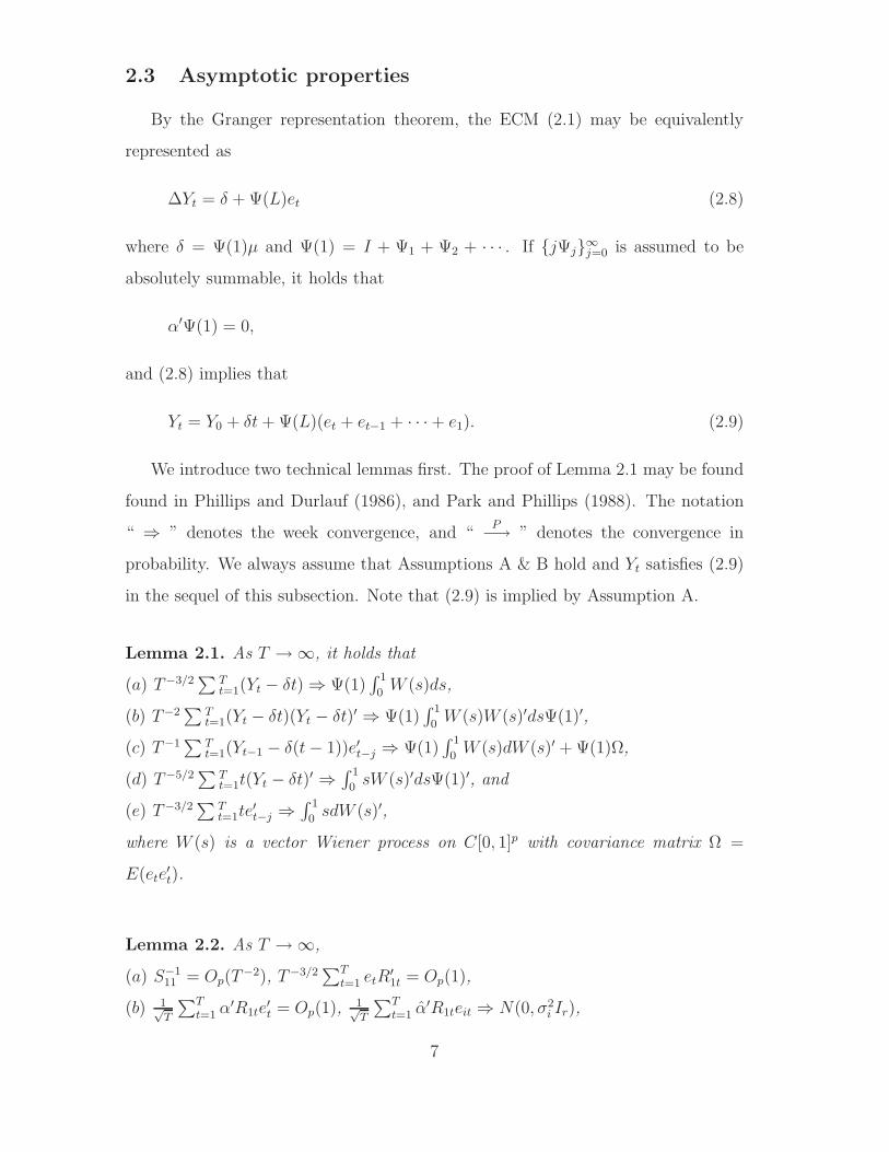
2.3 Asymptotic properties

By the Granger representation theorem, the ECM (2.1) may be equivalently

represented as

∆Yt = δ + Ψ(L)et (2.8)

where δ = Ψ(1)µ and Ψ(1) = I + Ψ1 + Ψ2 + · · · . If jΨj∞j=0 is assumed to be

absolutely summable, it holds that

α′Ψ(1) = 0,

and (2.8) implies that

Yt = Y0 + δt+ Ψ(L)(et + et−1 + · · · + e1). (2.9)

We introduce two technical lemmas first. The proof of Lemma 2.1 may be found

found in Phillips and Durlauf (1986), and Park and Phillips (1988). The notation

“ ⇒ ” denotes the week convergence, and “P−→ ” denotes the convergence in

probability. We always assume that Assumptions A & B hold and Yt satisfies (2.9)

in the sequel of this subsection. Note that (2.9) is implied by Assumption A.

Lemma 2.1. As T → ∞, it holds that

(a) T−3/2∑

Tt=1(Yt − δt) ⇒ Ψ(1)

∫ 1

0W (s)ds,

(b) T−2∑

Tt=1(Yt − δt)(Yt − δt)′ ⇒ Ψ(1)

∫ 1

0W (s)W (s)′dsΨ(1)′,

(c) T−1∑

Tt=1(Yt−1 − δ(t− 1))e′t−j ⇒ Ψ(1)

∫ 1

0W (s)dW (s)′ + Ψ(1)Ω,

(d) T−5/2∑

Tt=1t(Yt − δt)′ ⇒

∫ 1

0sW (s)′dsΨ(1)′, and

(e) T−3/2∑

Tt=1te

′t−j ⇒

∫ 1

0sdW (s)′,

where W (s) is a vector Wiener process on C[0, 1]p with covariance matrix Ω =

E(ete′t).

Lemma 2.2. As T → ∞,

(a) S−111 = Op(T

−2), T−3/2∑T

t=1 etR′1t = Op(1),

(b) 1√T

∑Tt=1 α

′R1te′t = Op(1), 1√

T

∑Tt=1 α

′R1teit ⇒ N(0, σ2i Ir),

7

(c) α′S11αP→ Σ11, α

′S11α = Op(1), where Σ11 is some positive definite matrix, and

(d) VTP→ V , where VT = diag(λ1T , λ1T , . . . , λrT ) and V = diag(λ1, λ2, . . . , λr),

λ1T ≥ · · · ≥ λrT be the r largest generalized eigenvalues of S10S01 with respect to

S11, and λ1 ≥ · · · ≥ λr > 0 are constants.

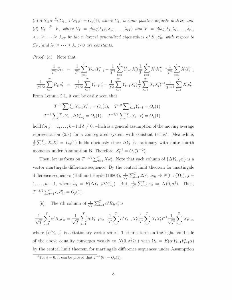
Proof. (a) Note that

1

T 2S11 =

1

T 3

T∑

t=1

Yt−1Y′t−1 −

1

T 2

T∑

t=1

Yt−1X′t(

1

T

T∑

t=1

XtX′t)

−1 1

T 2

T∑

t=1

XtY′t−1

1

T 3/2

T∑

t=1

R1te′t =

1

T 3/2

T∑

t=1

Yt−1e′t −

1

T 2

T∑

t=1

Yt−1X′t(

1

T

T∑

t=1

XtX′t)

−1 1

T 1/2

T∑

t=1

Xte′t.

From Lemma 2.1, it can be easily seen that

T−3∑

Tt=1Yt−1Y

′t−1 = Op(1), T−2

∑

Tt=1Yt−1 = Op(1)

T−2∑

Tt=1Yt−1∆Y

′t−j = Op(1), T−3/2

∑

Tt=1Yt−1e

′t = Op(1)

hold for j = 1, . . . , k−1 if δ 6= 0, which is a general assumption of the moving average

representation (2.8) for a cointegrated system with constant terms2. Meanwhile,

1T

∑Tt=1XtX

′t = Op(1) holds obviously since ∆Yt is stationary with finite fourth

moments under Assumption B. Therefore, S−111 = Op(T

−2).

Then, let us focus on T−1/2∑T

t=1Xte′t. Note that each column of ∆Yt−je

′t is a

vector martingale difference sequence. By the central limit theorem for martingale

difference sequences (Hall and Heyde (1980)), 1√T

∑Tt=1 ∆Yt−jeit ⇒ N(0, σ2

i Ω1), j =

1, . . . , k − 1, where Ω1 = E(∆Yt−j∆Y′t−j). But, 1√

T

∑Tt=1 eit ⇒ N(0, σ2

i ). Then,

T−3/2∑T

t=1 etR′1t = Op(1).

(b) The ith column of 1√T

∑Tt=1 α

′R1te′t is

1√T

T∑

t=1

α′R1teit =1√T

T∑

t=1

α′Yt−1eit−1

T

T∑

t=1

α′Yt−1X′t(

1

T

T∑

t=1

XtX′t)

−1 1√T

T∑

t=1

Xteit,

where α′Yt−1 is a stationary vector series. The first term on the right hand side

of the above equality converges weakly to N(0, σ2i Ω0) with Ω0 = E(α′Yt−1Y

′t−1α)

by the central limit theorem for martingale difference sequences under Assumption

2For δ = 0, it can be proved that T−1S11 = Op(1).

8

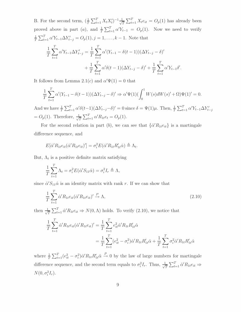
B. For the second term, ( 1T

∑Tt=1XtX

′t)

−1 1√T

∑Tt=1 Xteit = Op(1) has already been

proved above in part (a), and 1T

∑Tt=1 α

′Yt−1 = Op(1). Now we need to verify

1T

∑Tt=1 α

′Yt−1∆Y′t−j = Op(1), j = 1, . . . , k − 1. Note that

1

T

T∑

t=1

α′Yt−1∆Y′t−j =

1

T

T∑

t=1

α′(Yt−1 − δ(t− 1))(∆Yt−j − δ)′

+1

T

T∑

t=1

α′δ(t− 1)(∆Yt−j − δ)′ +1

T

T∑

t=1

α′Yt−1δ′.

It follows from Lemma 2.1(c) and α′Ψ(1) = 0 that

1

T

T∑

t=1

α′(Yt−1 − δ(t− 1))(∆Yt−j − δ)′ ⇒ α′Ψ(1)(

∫ 1

0

W (s)dW (s)′ +Ω)Ψ(1)′ = 0.

And we have 1T

∑Tt=1 α

′δ(t−1)(∆Yt−j−δ)′ = 0 since δ = Ψ(1)µ. Then, 1T

∑Tt=1 α

′Yt−1∆Y′t−j

= Op(1). Therefore, 1√T

∑Tt=1 α

′R1tet = Op(1).

For the second relation in part (b), we can see that α′R1teit is a martingale

difference sequence, and

E[α′R1teit(α′R1teit)

′] = σ2iE(α′R1tR

′1tα) , Λt.

But, Λt is a positive definite matrix satisfying

1

T

T∑

t=1

Λt = σ2iE(α′S11α) = σ2

i Ir , Λ,

since α′S11α is an identity matrix with rank r. If we can show that

1

T

T∑

t=1

α′R1teit(α′R1teit)

′ P→ Λ, (2.10)

then 1√T

∑Tt=1 α

′R1teit ⇒ N(0,Λ) holds. To verify (2.10), we notice that

1

T

T∑

t=1

α′R1teit(α′R1teit)

′ =1

T

T∑

t=1

e2itα′R1tR

′1tα

=1

T

T∑

t=1

(e2it − σ2i )α

′R1tR′1tα +

1

T

T∑

t=1

σ2i α

′R1tR′1tα

where 1T

∑Tt=1(e

2it − σ2

i )α′R1tR

′1tα

P→ 0 by the law of large numbers for martingale

difference sequence, and the second term equals to σ2i Ir. Thus, 1√

T

∑Tt=1 α

′R1teit ⇒N(0, σ2

i Ir).

9

(c) Since

α′S11α =1

T

T∑

t=1

α′Yt−1Y′t−1α− 1

T

T∑

t=1

α′Yt−1X′t(

1

T

T∑

t=1

XtX′t)

−1 1

T

T∑

t=1

XtY′t−1α,

using Lemma 2.1 again and noticing that α′Ψ(1) = 0, α′δ = 0, and α′Yt−1 is station-

ary, we have α′S11αP→ Σ11.

For the second relation in part (c), lettingR1 be the T×pmatrix [R11, R12, · · · , R1T ]′,

we have

‖α′S11α‖ = ‖α′R′1R1

Tα‖ ≤ ‖α′R

′1R1

Tα‖1/2‖α′R

′1R1

Tα‖1/2

= ‖α′S11α‖1/2‖α′S11α‖1/2 = Op(1).

(d) The proof of this part is omitted because it is similar to that given by

Johansen (1988, 1991).

Now we present the asymptotic normality of α in the theorem below.

Theorem 2.1. There exists a r × r invertible matrix HT for which

√T (α− αHT ) = Op(1)

as T → ∞. Furthermore, for each 1 ≤ i ≤ r,

√T (αi − αHiT ) = αγ′

1√T

T∑

t=1

etR′1tαiλ

−1iT + op(1) ⇒ N(0, λ−2

i αγ′Ωγα′),

where Ω = E(ete′t), HiT is the i-th column of HT and λiT is the i-th largest general-

ized eigenvalue of S10S01 with respect to S11.

Proof. Recall the definition of VT = diag(λ1T , λ2T , . . . , λrT ). We have S10S01α =

S11αVT or equivalently S−111 S10S01αV

−1T = α. Take HT = γ′γα′S11αV

−1T , which is an

invertible matrix. Expanding S10S01 by using the fact S01 = γα′S11 + 1T

∑Tt=1 etR

′1t,

we can obtain

α− αHT = (αγ′1

T

T∑

t=1

etR′1tα+ S−1

11

1

T

T∑

t=1

R1te′tγα

′S11α

+S−111

1

T

T∑

t=1

R1te′t

1

T

T∑

t=1

etR′1tα)V −1

T . (2.11)

10

By Lemma 2.2, 1T

∑Tt=1 etR

′1tα = Op(1/

√T ), S−1

11 = Op(1/T2), 1

T

∑Tt=1R1te

′t =

Op(√T ), α′S11α = Op(1) and V −1

T = Op(1), it follows that

α− αHT = Op(1√T

) +Op(1√T 3

) +Op(1

T 2).

Thus,√T (α−αHT ) = Op(1), and the asymptotic distribution of each cointegrating

vector αi is determined by the first term on the right hand side of (2.11). We have

√T (αi − αHiT ) = αγ′

1√T

T∑

t=1

etR′1tαiλ

−1iT + op(1) ⇒ N(0, λ−2

i αγ′Ωγα′)

as stated, where λiTP→ λi by Lemma 2.2(d) and 1√

T

∑Tt=1 etR

′1tαi ⇒ N(0,Ω) can be

proved similarly to the second part of Lemma 2.2(b).

Theorem 2.1 implies that α is a consistent estimator of αHT for an invertible

matrix HT . In the theorem below, we show that γ ≡ S01α is a√T−consistent

estimator of γ(H ′T )−1 and Γ0 ≡ γα′ is a

√T−consistent estimator of Γ0 = γα′.

Theorem 2.2.√T (γ − γ(H ′

T )−1) = Op(1),√T (Γ0 − Γ0) = Op(1)

Proof. Note γ = S01α = (γα′S11 + 1T

∑Tt=1 etR

′1t)α and α′S11α = Ir. It holds that

γ − γ(H ′T )−1 = γ(α− αH−1

T )′S11α +1

T

T∑

t=1

etR′1tα.

The second term is Op(1/√T ) by Lemma 2.2(b). But, the first term can be rewritten

as −γ(H ′T )−1(α− αHT )′S11α. From the expression of α− αHT in (2.11), we have

α′S11(α− αHT ) = (α′S11αγ′ 1

T

T∑

t=1

etR′1tα +

1

T

T∑

t=1

α′R1te′tγα

′S11α

+1

T

T∑

t=1

α′R1te′t

1

T

T∑

t=1

etR′1tα)V −1

T . (2.12)

But, for HT = γ′γ(α′S11α)V −1T , it holds that H−1

T = Op(1), because VT converges

to a positive definite matrix V and α′S11α = Op(1) has full rank. It follows that

(α− αHT )′S11α = Op(1/√T ). Thus,

√T (γ − γ(H ′

T )−1) = Op(1).

11

Consider the second relation now. It holds that

Γ0 − Γ0 = γα′ − γα′

= (γ − γ(H ′T )−1)(α− αHT )′ + (γ − γ(H ′

T )−1)H ′Tα

′ + γ(H ′T )−1(α− αHT )′

= Op(1

T) +Op(

1√T

) +Op(1√T

) = Op(1√T

).

This completes the proof of Theorem 2.2.

Remark. From Theorem 2.1, the asymptotic covariance matrix of αi is λ−2i Γ′

0ΩΓ0.

It admits a consistent estimator λ−2iT Γ′

0(1T

∑Tt=1 ete

′t)Γ0, where

et =1

T

T∑

t=1

(∆Yt − Θ(Γ0)Xt − Γ0Yt−1)′(∆Yt − Θ(Γ0)Xt − Γ0Yt−1).

3 Estimation of the Cointegration Rank

Let r0 be the true value of the cointegration rank of model (2.1). In this section,

we discuss how to estimate r0 based on the estimated cointegration vector α derived

in section 2. The basic idea is to treat the rank as part of the “order” of model (2.1)

and to determine the order in terms of an appropriate information criterion. In this

section we always assume that Assumptions A and B hold. First we deal with the

case when the lag order k is known.

3.1 Determining the cointegration rank r with the lag order

k given

Consider the sum of squared residuals

R(r, α) = minγ

1

T

T∑

t=1

(R0t − γα′R1t)′(R0t − γα′R1t)

= tr(S00 − S01α(α′S11α)−1α′S10).

(3.1)

To avoid possible overfitting, we add a penalty term. Our penalized goodness-of-fit

criterion is defined as

M(r) = R(r, α) + nrg(T ), (3.2)

12

where g(T ) is the penalty for “overfitting” and nr is the number of freely estimated

parameters. Note that nr = p + p2(k − 1) + 2pr − r2 for model (2.1). We may

estimate r0 by minimizing

r = arg min0≤r≤p

M(r).

The following theorem shows that r is a consistent estimator of r0 provided that the

penalty function g(T ) satisfies some mild conditions.

Theorem 3.1. As T → ∞, rP→ r0 provided that g(T ) → 0 and Tg(T ) → ∞.

The theorem above shows that both the BIC criterion with g(T ) = ln(T )/T

(Schwarz 1978) and the HQ criterion with g(T ) = 2 ln(ln(T ))/T (Hannan and Quinn

1979) lead to consistent estimators for the cointegration order. To prove Theorem

3.1, we need a slightly generalized form of Theorem 2.1.

Lemma 3.1. For any 1 ≤ r ≤ p, there exists a r0 × r matrix HrT with full rank such

that, as T → ∞

√T (α− αHr

T )VT = Op(1).

Proof. The proof is the same as that of Theorem 2.1 without any modification,

except that VT is not necessarily invertible and HrTVT = γ′γα′S11α is not a square

matrix anymore if r 6= r0. The reason is that r0 denotes the true rank of γ and α

now.

Let Al denote a matrix with rank l. In particular, αr0 and αr (1 ≤ r ≤ p) denote

the matrices α and α with ranks r0 and r respectively.

Lemma 3.2. For any r0 ≤ r ≤ p, R(r, αr) − R(r0, αr0) = Op(

1T).

Proof. Since

|R(r, αr) − R(r0, αr0)| ≤ |R(r, αr) − R(r0, α

r0)| + |R(r0, αr0) − R(r0, α

r0)|

≤ 2 maxr0≤r≤p

|R(r, αr) − R(r0, αr0)|,

13

then, it is sufficient to prove for any r0 ≤ r ≤ p,

R(r, αr) − R(r0, αr0) = Op(T

−1).

Notice that S01 = γαr′0S11 + 1

T

∑Tt=1 etR

′1t and

R(r, αr) = tr(S00 − S01αr(αr′S11α

r)−1αr′S10),

R(r0, αr0) = tr(S00 − S01α

r0(αr′0S11α

r0)−1αr′0S10).

We have

R(r, αr) − R(r0, αr0)

=tr[γαr′0S11α

r0γ′ − γαr′0S11α

rαr′S11αr0γ′]

+ 2tr[1

T

T∑

t=1

γαr′0R1te

′t − γαr′

0S11αr 1

T

T∑

t=1

αr′R1te′t]

+ tr[1

T

T∑

t=1

etR′1tα

r0(αr′0S11α

r0)−1 1

T

T∑

t=1

αr′0R1te

′t −

1

T 2

T∑

t=1

etR′1tα

rT

∑

t=1

αr′R1te′t]

=I + II + III.

It follows straightly from Lemma 2.2(b) and (c) that III = Op(1T).

Now, for r ≥ r0, HrTVT = γ′γαr′

0S11αr has rank r0. Let Hr+

T denote the gen-

eralized inverse of HrT such that Hr

THr+T = Ir0

, then it can be written as Hr+T =

VT (αr′0S11α

r)r+(γ′γ)−1. It follows that,

I = tr[γHr+′

T (αr − αr0HrT )′S

1/211 (Ip − S

1/211 α

rαr′S1/211 )S

1/211 (αr − αr0Hr

T )Hr+T γ′]

where Ip is an identity matrix with rank p. Furthermore, it is easy to see that

Ip − S1/211 α

rαr′S1/211 is an idempotent matrix with eigenvalues 0 or 1. Because of the

inequality x(Ip − S1/211 α

rαr′S1/211 )x′ ≤ xx′ for any vector x,

I ≤p

∑

i=1

γ′iHr+′

T (αr − αr0HrT )′S11(α

r − αr0HrT )Hr+

T γi

=

p∑

i=1

γ′i(γ′γ)−1(αr′

0S11αr)r+′

V ′T (αr − αr0Hr

T )′S11(αr − αr0Hr

T )VT (αr′0S11α

r)r+(γ′γ)−1γi

where γ′i is the ith column of γ. From the expression of (αr −αr0HrT )VT in (2.11), it

follows that V ′T (αr−αr0Hr

T )′S11(αr−αr0Hr

T )VT = Op(1T). Additionally, (αr′

0S11αr)r+ =

14

Op(1) because αr′0S11α

r = Op(1) has full rank3 r0 by Lemma 2.2(c). Hence, I =

Op(1T).

For II, we have

II =2tr[

γHr+′

T [(αr − αr0HrT )′S11α

r 1

T

T∑

t=1

αr′R1te′t − (αr − αr0Hr

T )′1

T

T∑

t=1

R1te′t]]

=2tr[

γ(γ′γ)−1(αr′0S11α

r)r+′

[V ′T (αr − αr0Hr

T )′S11αr 1

T

T∑

t=1

αr′R1te′t

− V ′T (αr − αr0Hr

T )′1

T

T∑

t=1

R1te′t]]

.

By using the expression of (αr−αr0HrT )VT in (2.11) and Lemma 2.2 again, we obtain

that V ′T (αr − αr0Hr

T )′S11αr = Op(

1√T) and V ′

T (αr − αr0HrT )′ 1

T

∑Tt=1R1te

′t = Op(

1T).

The details are similar to those for (2.12). Finally, the facts αr′0S11α

r = Op(1) and

1T

∑Tt=1 α

r′R1te′t = Op(

1√T) imply that II = Op(

1T). This completes the proof of

Lemma 3.2.

Proof of Theorem 3.1. The objective is to verify that limT→∞ P (M(r)−M(r0) <

0) = 0 for all r ≤ p and r 6= r0, where

M(r) − M(r0) = R(r, αr) − R(r0, αr0) − (nr0

− nr)g(T ).

For r < r0, from (3.1), we have R(r, αr)− R(r0, αr0) =

∑r0

i=r+1 λiT , where λiT is the

ith generalized eigenvalue of S10S01 respect to S11 in decreasing order. Therefore, if

g(T ) → 0 as T → ∞,

P (M(r) − M(r0) < 0) = P (

r0∑

i=r+1

λiT < (r0 − r)(2p− (r0 + r))g(T ))

→ P (

r0∑

i=r+1

λi < 0) = 0

by Lemma 2.2 (d) that λiTP→ λi > 0.

3The limit of αr′

0S11αr can be established in a similar way to that of Proposition 1 in Bai (2003)

(with p fixed).

15

For r > r0, Lemma 3.2 implies that R(r0, αr0) − R(r, αr) = Op(

1T). Thus, if

Tg(T ) → ∞ as T → ∞, we have

P (M(r) − M(r0) < 0) = P (R(r0, αr0) − R(r, αr) > (r − r0)(2p− (r + r0))g(T ))

= P (T [R(r0, αr0) − R(r, αr)] > (r − r0)(2p− (r + r0))Tg(T ))

→ 0.

The proof of Theorem 3.1 is completed.

3.2 Determining the cointegration rank r and the lag order

k jointly

One of the important issues in applying ECM is to determine the lag order k.

Johansen (1991) adopted a two-step procedure as follows: first the lag order k is

determined by either an appropriate information criterion or a sequence of likelihood

ratio test, and then the cointegration rank r is determined by an LRT. We proceed

differently below and determine both r and k simultaneously by minimizing an

appropriate penalized goodness-of-fit criterion.

Put

M(r, k) = R(r, k, αrk) + nr,kg(T ), (3.3)

where R(r, k, αrk) and nr,k are the same, respectively, as R(r, αr

k) and nr in (3.2) in

which k is suppressed. We determine both the cointegration rank and the lag order

as follows:

(r, k) = arg min0≤r≤p,1≤k≤K

M(r, k),

where K is a prescribed positive integer. Let k0 be the true lag order of model (2.1).

The theorem below ensures that (r, k) is a consistent estimtor for (r0, k0).

Theorem 3.2. As T → ∞, (r, k)P→ (r0, k0) provided that g(T ) → 0 and Tg(T ) → ∞.

16

We denote ECM with different lag orders (k1 < k2) as

Modelk1: ∆Yt = γα′Yt−1 + ΘXt + et (3.41)

Modelk2: ∆Yt = γα′Yt−1 + ΘXt + Θ1Zt + et (3.42)

with Θ = (µ,Γ1, . . . ,Γk1−1), Θ1 = (Γk1, . . . ,Γk2−1), Xt = (1,∆Y ′

t−1, . . . ,∆Y′t−k1+1)

′,

Zt = (∆Y ′t−k1

, . . . ,∆Y ′t−k2+1)

′.

Lemma 3.3. For any 1 ≤ k1 < k2,

if Modelk1is true, R(r0, k1, α

r0

k1) − R(r0, k2, α

r0

k2) = Op(

1T);

if Modelk2is true, p limT→∞[R(r0, k1, α

r0

k1) − R(r0, k2, α

r0

k2)] > 0, where p lim de-

notes the limit in probability.

Proof. From the expression of R(r, α) in (3.1) and the following matrix identity

(

X ′1 X ′

2

)

A B

B′ D

−1

Y1

Y2

= X ′1A

−1Y1 + (X ′2 −X ′

1A−1B)(D −B′A−1B)−1(Y2 −B′A−1Y1),

(3.5)

it can be seen that

R(r0, k1, αr0

k1) = tr(S00 − S01α

r0

k1(αr0

k1

′S11αr0

k1)−1αr0

k1

′S10),

R(r0, k2, αr0

k2) = tr(S00 −

(

S01αr0

k1S02

)

αr0

k1

′S−111 α

r0

k1αr0

k1

′S12

S21αr0

k1S22

−1

αr0

k1

′S10

S20

)

where Sij = 1T

∑Tt=1 RitR

′jt for i, j = 0, 1, 2, R2t = Zt −

∑Tt=1 ZtX

′t(

∑Tt=1 XtX

′t)

−1Xt,

R1t = Yt−1−∑T

t=1 Yt−1X′t(

∑Tt=1XtX

′t)

−1Xt, andR0t = ∆Yt−∑T

t=1 ∆YtX′t(

∑Tt=1XtX

′t)

−1Xt.

Therefore,

R(r0, k1, αr0

k1) − R(r0, k2, α

r0

k2)

=tr[(S02 − S01αr0

k1(αr0

k1

′S11αr0

k1)−1αr0

k1

′S12)

(S22 − S21αr0

k1(αr0

k1

′S11αr0

k1)−1αr0

k1

′S12)−1(S20 − S21α

r0

k1(αr0

k1

′S11αr0

k1)−1αr0

k1

′S10)].

(3.6)

If the model with lag order k1 is true, putting the estimator of Θ defined in

section 2 into Modelk1, we obtain that R0t = γαr0

k1

′R1t + et, and

S02 = γαr0

k1

′S12 + 1T

∑Tt=1 etR

′2t = γαr0

k1

′S12 +Op(1√T),

S02 − S01αr0

k1(αr0

k1

′S11αr0

k1)−1αr0

k1

′S12 = (γ − γ(αr0

k1))αr0

k1

′S12 +Op(1√T) = Op(

1√T).

17

Since et, ∆Yt and αr0

k1

′Yt−1 are stationary sequences, it follows that 1T

∑Tt=1 etR

′2t =

Op(1√T) and αr0

k1

′S12 = Op(1) by the similar way to that of Lemma 2.2. For the term

(γ − γ(αr0

k1)), we have

γ − γ(αr0

k1) =γ − S01α

r0

k1(αr0

k1

′S11αr0

k1)−1

=γ − (γαr0

k1

′S11 + T−1

T∑

t=1

etR′1t)α

r0

k1(αr0

k1

′S11αr0

k1)−1

= − T−1T

∑

t=1

etR′1tα

r0

k1(αr0

k1

′S11αr0

k1)−1 = Op(1/

√T ).

The last equality holds by Lemma 2.2 (b) and (c). It is easy to find that S22 = Op(1),

and then

S22 − S21αr0

k1(αr0

k1

′S11αr0

k1)−1αr0

k1

′S12 = Op(1).

Then, it follows that R(r0, k1, αr0

k1) − R(r0, k2, α

r0

k2) = Op(

1T).

If the model with lag order k2 is true, denoting the limits of

S02 − S01αr0

k1(αr0

k1

′S11αr0

k1)−1αr0

k1

′S12 and S22 − S21αr0

k1(αr0

k1

′S11αr0

k1)−1αr0

k1

′S12

by E and G respectively, we argue that tr(EG−1E ′) > 0 by the similar way to that

given by Aznar and Salvador (2002). Hence, by (3.6), p limT→∞[R(r0, k1, αr0

k1) −

R(r0, k2, αr0

k2)] > 0.

Proof of Theorem 3.2. The goal is to verify that P (r = r0, k = k0) → 1 as

T → ∞. Note that we have established the consistency of r for any fixed lag order

k in Theorem 3.1, which implies that P (r = r0) → 1 as T → ∞. Thus, it remains

to prove that P (k = k0|r = r0) → 1, or equivalently, for all 1 ≤ k ≤ K and k 6= k0,

limT→∞

P (M(r0, k) − M(r0, k0) < 0) = 0.

From the proof of Lemma 3.2, we have R(r0, k, αr0

k ) − R(r0, k, αr0

k ) = Op(1T) for

any k ≥ 1. Therefore,

M(r0, k) − M(r0, k0)

= R(r0, k, αr0

k ) − R(r0, k0, αr0

k0) + p2(k − k0)g(T )

= R(r0, k, αr0

k ) − R(r0, k0, αr0

k0) + p2(k − k0)g(T ) +Op(

1

T).

18

For k < k0, we have

P (M(r0, k) − M(r0, k0) < 0)

= P (R(r0, k, αr0

k ) − R(r0, k0, αr0

k0) +Op(

1

T) < p2(k0 − k)g(T )) → 0

if g(T ) → 0 as T → ∞, because R(r0, k, αr0

k )−R(r0, k0, αr0

k0) > 0 has a positive limit

by Lemma 3.3.

For k > k0, Lemma 3.3 implies that R(r0, k0, αr0

k0)−R(r0, k, α

r0

k ) = Op(1T). Thus,

if Tg(T ) → ∞ as T → ∞, we have

P (M(r0, k) − M(r0, k0) < 0)

= P (T [R(r0, k0, αr0

k0) − R(r0, k, α

r0

k )] +Op(1) > p2(k − k0)Tg(T )) → 0.

The proof is completed.

4 Numerical properties

4.1 Simulated examples

Two experiments are conducted to examine the finite sample performance of

the proposed criteria (3.2) and (3.3). The comparisons with the LRT approach of

Johansen (1991) and the information criterion of Aznar and Salvador (2002) are also

made. It is easy to see from Theorems 3.1 and 3.2 that the choice of the penalty

function g(·) is flexible. It may take a general form:

g(T ) = ξ ln(T )/T + 2η ln(ln(T ))/T, ξ ≥ 0, η ≥ 0, (4.1)

which reduces to the BIC of Schwarz (1978) with ξ = 1 and η = 0, to the HQIC

of Hannan and Quinn (1979) with ξ = 0 and η = 1, and to the LCIC of Gonzalo

and Pitarakis (1998) with ξ = η = 12. We use the three concrete forms in our

experiments:

M1(r, k) = R(r, k, αrk) + nr,k ln(T )/T,

M2(r, k) = R(r, k, αrk) + 2nr,k lnln(T )/T,

M3(r, k) = R(r, k, αrk) + nr,k[ln(T )/6 + 4 lnln(T )/3]/T.

19

We set sample size at T = 30, 50, 100, 200, 300 or 400. For each setting, we replicate

the simulation 2000 times. The data are generated from the ECM (2.1) with either

independent errors following one of the four distributions below

et ∼ N(0, Ip), (4.1a)

et = εt + 10θεt, εt ∼ N(0, Ip), θ ∼ Poisson(τ), (4.1b)

eit ∼ t(q), (4.1c)

eit ∼ Cauchy, (4.1d)

or uncorrelated but dependend errors

eit = hitεit, h2it = ϕ0 + ϕ1e

2it−1 + ψ1h

2it−1, εit ∼ N(0, 1), (4.2)

ϕ0 > 0, ϕ1 ≥ 0, ψ1 ≥ 0, εit are independent for all i and t.

Distributions in (4.1b) - (4.1d) are heavy-tailed. In particular, (4.1b) is often used in

GARCH-Jump models for modelling asset prices. Note that for eit ∼ t(q), E|eit|q =

∞. Furthermore, (4.1d) represents an extreme situation with E|eit| = ∞, and

therefore it does not fulfill Assumption B. We include it to examine the robustness

of the methods against the assumption of the finite fourth moment.

First we generate data from model

y1t = µ+ 0.6y2t + e1t, ∆yit = µ+ eit for i = 2, 3. (4.3)

The cointegration rank r = 1 and the lag order k = 1. Assuming k = 1 is known but

both µ and the coefficient 0.6 are unknown, we estimate r by minimizing Mi(r, 1)

for i = 1, 2, 3 and also by the Johansen’s LRT approach. For each of different

settings, we draw 2000 samples from (4.3), the percentages of the samples resulting

the correct estimate (i.e. r = 1) are listed in Tables 1 – 5. Table 1 shows that even

with Gaussian errors, our method based on the criterion M3 outperforms the LRT

based method. When the sample size is small (i.e. T = 30 or 50), the methods using

M1 and M2 perform poorly. However the performance improves when T increases.

Also noticiable is the fact that the presence of a linear trend (i.e. µ 6= 0) deteriorates

20

slightly the performance of all the four methods. Tables 2 – 4 show that the method

based on M3 remains to perform better than the others when error distribution is

changed to (4.1b), (4.1c) and (4.1d), although the heavy tails of the error distribution

impact negatively to the performance of all the methods. Especially with Cauchy

errors, the percentages of the correct estimates are low for all the four method with

sample size T smaller than 100. But still the method based on M3 always performs

better than the other three. Table 5 indicates that the method based on M3 also

outperforms the others even with dependent ARCH(1) (i.e. ψ1 = 0) or GARCH(1,1)

errors (i.e. ψ1 6= 0).

Our second example concerns the model

∆y1t

∆y2t

=

0.5

0.5

+

0.3 0

0 0.5

∆y1t−1

∆y2t−1

+

0.4

0.6

(

1, −2)

y1t−1

y2t−1

+

e1t

e2t

.

(4.4)

We assume that all the coefficients in the models are unknown. We now estimate

the cointegration rank r(=1) and the lag order k(=2) by minimizing M3(r, k) with

the five different error distributions specified in (4.1a)-(4.1d) and (4.2). For the com-

parison purpose, we also compute Aznar and Salvador’s (2002) estimates obtained

by minimizing the information criterion (IC)

IC(r, k) = Tln |S00| +r

∑

i=1

ln(1 − λi) + nr,kg(T ),

where g(T ) = [ln(T )/6 + 4 lnln(T )/3]/T and λi is the i-th largest generalized

eigenvalue of S10S−100 S01 with respect to S11. The percentages of the correct estimates

(i.e. (r, k) = (1, 2)) in a simulation with 2000 replications are listed in Table 6.

Note that the above IC-criterion is based on a Gaussian likelihood function. It

is not surprising that it outperforms our method based on M3 when the errors

are Gaussian. However Table 6 also indicates that this IC-criterion is sensitive to

the normality assumption. In fact for all the four other error distributions, our

method based on M3 performed better. When the heaviness of the distribution tails

increases, the performance of the both methods decreases. We also note that both

the methods perform poorly when the sample size is as small as T = 30.

21

4.2 A real data example

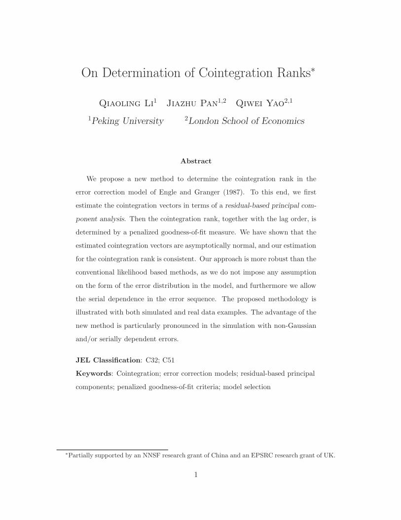
We consider the annual records of the GDP per capita, labor productivity per

person and labor productivity per hour of the Netherlands from 1950 to 20054. The

time plots of the logarithmic GDP (solid lines), the labor productivity per person

(dash-dotted lines) and the labor productivity per hour (dotted lines) are presented

in Figure 1. It indicates that there may exist a linear cointegrating relationship

among the three variables.

We determine the cointegration rank by minimising M3(r, k). The surface of

M3(r, k) is plotted against r and k in Figure 2. The minimal point of the surface

is attained at (r, k) = (1, 2), leading to a fitted ECM model (2.1) for this data set

with the lag order 2 and the cointegrating rank 1. The estimate of the cointegrating

vector with the first component normalized to one is α = (1.00, 3.82,−3.28)′. The

other estimated coefficients in model (2.1) are as follows

µ = (9.09, 10.09, 2.41)′, γ = −(0.23, 0.25, 0.06)′,

Γ1 =

0.20 −0.32 0.60

−0.36 0.19 0.55

−0.48 0.32 0.46

.

REFERENCES

Anderson, T. W. (1951) Estimating linear restrictions on regression coffcients for

multivariate normal distributions. Annals of Mathematical Statistics 22, 327-

351.

Ahn, S. K. & G. C. Reinsel (1988) Nested reduced-rank autoregressive models

for multiple time series. Journal of the American Statistical Association 83,

849-856.

4Data source: The Conference Board and Groningen Growth and Development Center, Total

Economy Database, January 2006, http://www.ggdc.net.

22

Ahn, S. K. & G. C. Reinsel (1990) Estimation for partially nonstationary multi-

variate autoregressive models. Journal of the American Statistical Association

85, 813-823.

Aznar, A. & M. Salvador (2002) Selecting the rank of the cointegration space and

the form of the intercept using an information criterion. Econometric Theory

18, 926-947.

Bai, J. S. (2003) Inferential theory for factor models of large dimensions. Econo-

metrica 71, 926-947.

Engle, R. F. & C. W. J. Granger (1987) Co-integration and error correction: Rep-

resentation, estimation and testing. Econometrica 55, 251-276.

Gonzalo, J. (1994) Five alternative methods of estimating long-run equilibrium

relationships Journal of Econometrics 60, 203-233.

Gonzalo, J. & T. H. Lee (1998) Pitfalls in testing for long-run relationships. Journal

of Econometrics 86, 129-154.

Gonzalo, J. & J. Y. Pitarakis (1998) Specification via model selection in vector

error correction models. Economics Letters 60, 321C328.

Granger, C. W. J. (1981) Some properties of time series data and their use in

econometric model specification. Journal of Econometrics 16, 121-130.

Granger, C. W. J. & A. A. Weiss (1983) Time series analysis of error correction

models, in Studies in Econometrics, Time Series and Multivariate Statistics,

ed. by S. Karlin, T. Amemiya and L.A. Goodman. New York: Academic

Press, 255-278.

Hall, P. & C. C. Heyde (1980). Martingale Limit Theory and Its Applications.

Academic Press, New York.

Hannan, E. & B. Quinn (1979) The determination of the order of an autoregression.

Journal of the Royal Statistical Society, Ser. B 41, 190-195.

23

Huang, B. N. & C. W. Yang (1996) Long-run purchasing power parity revisited: a

monte carlo simulation. Applied Economics 28, 967-974.

Johansen, S. (1988) Statistical analysis of cointegration vectors. Journal of Eco-

nomic Dynamics and Control 12, 231-254.

Johansen, S. (1991) Estimation and hypothesis testing of cointegration vectors in

Gaussian vector autoregressive models. Econometrica 59, 1551-1580.

Kapetanios, G. (2004) The asymptotic distribution of the cointegration rank esti-

mator under the Akaike Information Criterion. Econometric Theory 20, 735-

742.

Park, J. Y. & P. C. B. Phillips (1988) Statistical inference in regressions with

integrated processes: Part 1. Econometric Theory 4, 468-497.

Phillips, P. C. B. (1991) Optimal inference in cointegrated systems. Econometrica

59, 283-306.

Phillips, P. C. B. & S. N. Durlauf (1986) Multiple time series regression with

integrated processes. The Review of Economic Studies 53, 473-495.

Schwarz, G. (1978) Estimating the dimension of a model. Annals of Statistics 6,

461-464.

Stock, J. H. (1987) Asymptotic properties of least squares estimators of cointegrat-

ing vectors. Econometrica 55, 1035-1056.

Stock, J. H. & M. Watson (1988) Testing for common trends. Journal of the

American Statistical Association 83, 1097-1107.

Wang, Zijun. & D. Bessler (2005) A monte carlo study on the selection of cointe-

grating rank using information criteria. Econometric Theory 21, 593-620.

24

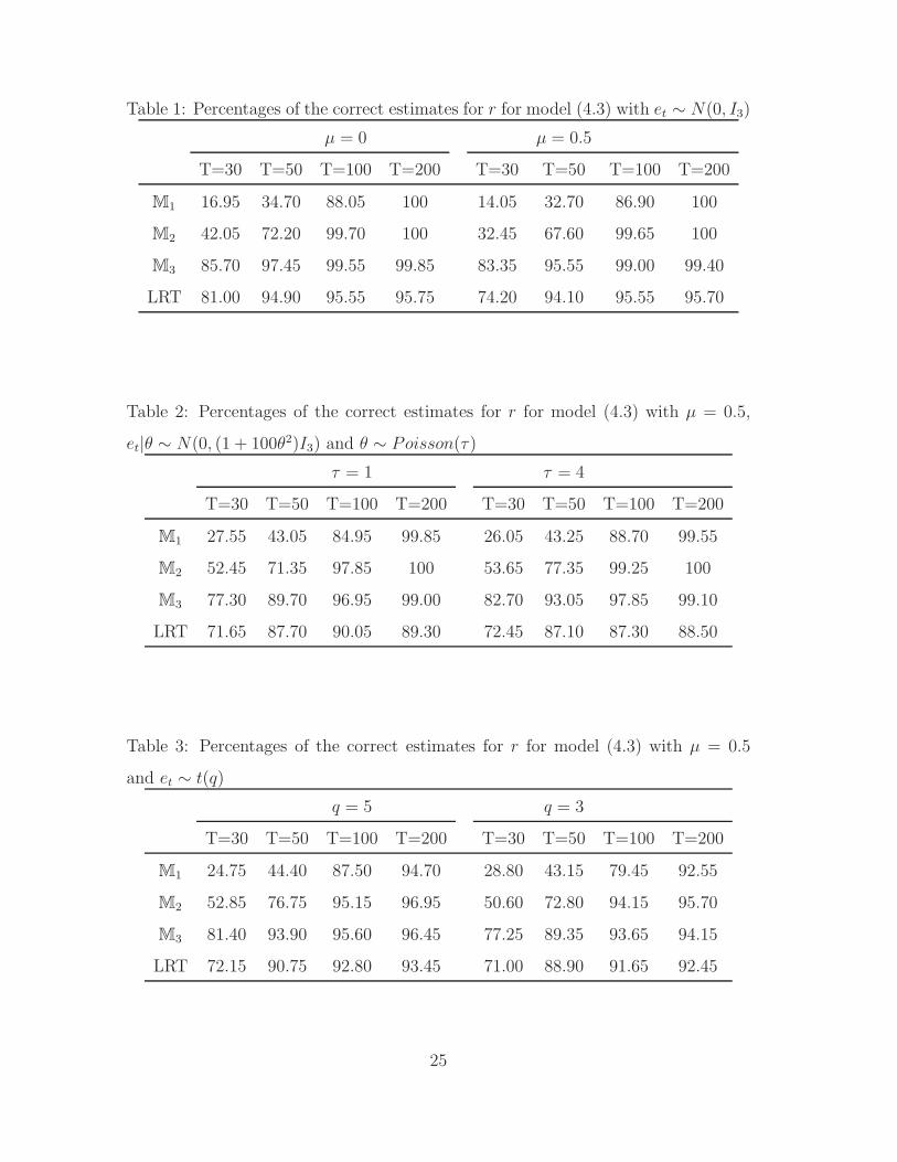
Table 1: Percentages of the correct estimates for r for model (4.3) with et ∼ N(0, I3)

µ = 0 µ = 0.5

T=30 T=50 T=100 T=200 T=30 T=50 T=100 T=200

M1 16.95 34.70 88.05 100 14.05 32.70 86.90 100

M2 42.05 72.20 99.70 100 32.45 67.60 99.65 100

M3 85.70 97.45 99.55 99.85 83.35 95.55 99.00 99.40

LRT 81.00 94.90 95.55 95.75 74.20 94.10 95.55 95.70

Table 2: Percentages of the correct estimates for r for model (4.3) with µ = 0.5,

et|θ ∼ N(0, (1 + 100θ2)I3) and θ ∼ Poisson(τ)

τ = 1 τ = 4

T=30 T=50 T=100 T=200 T=30 T=50 T=100 T=200

M1 27.55 43.05 84.95 99.85 26.05 43.25 88.70 99.55

M2 52.45 71.35 97.85 100 53.65 77.35 99.25 100

M3 77.30 89.70 96.95 99.00 82.70 93.05 97.85 99.10

LRT 71.65 87.70 90.05 89.30 72.45 87.10 87.30 88.50

Table 3: Percentages of the correct estimates for r for model (4.3) with µ = 0.5

and et ∼ t(q)

q = 5 q = 3

T=30 T=50 T=100 T=200 T=30 T=50 T=100 T=200

M1 24.75 44.40 87.50 94.70 28.80 43.15 79.45 92.55

M2 52.85 76.75 95.15 96.95 50.60 72.80 94.15 95.70

M3 81.40 93.90 95.60 96.45 77.25 89.35 93.65 94.15

LRT 72.15 90.75 92.80 93.45 71.00 88.90 91.65 92.45

25

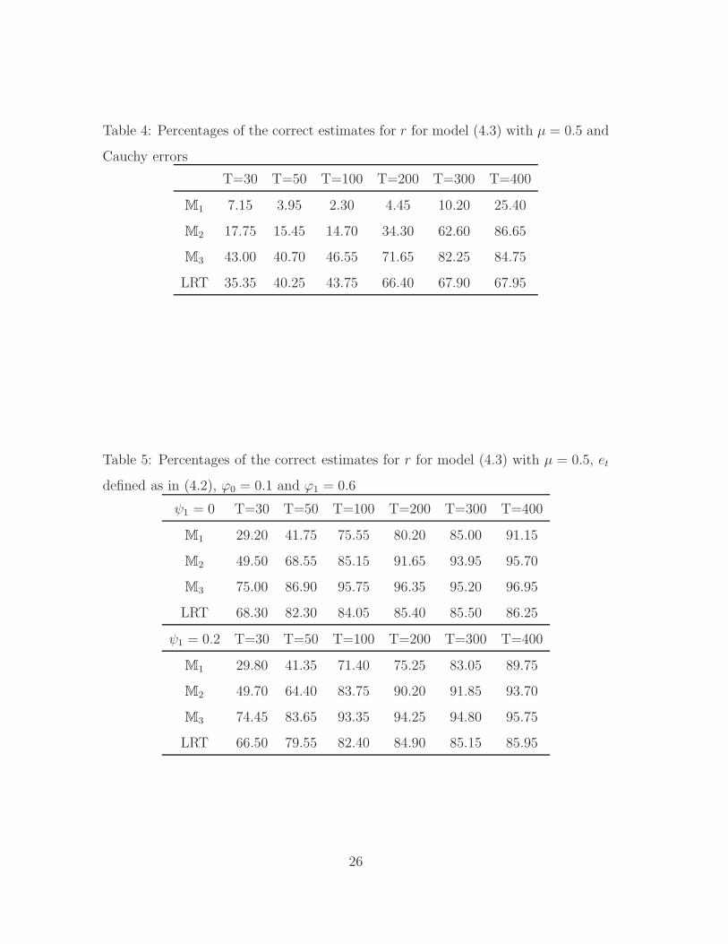
Table 4: Percentages of the correct estimates for r for model (4.3) with µ = 0.5 and

Cauchy errors

T=30 T=50 T=100 T=200 T=300 T=400

M1 7.15 3.95 2.30 4.45 10.20 25.40

M2 17.75 15.45 14.70 34.30 62.60 86.65

M3 43.00 40.70 46.55 71.65 82.25 84.75

LRT 35.35 40.25 43.75 66.40 67.90 67.95

Table 5: Percentages of the correct estimates for r for model (4.3) with µ = 0.5, et

defined as in (4.2), ϕ0 = 0.1 and ϕ1 = 0.6

ψ1 = 0 T=30 T=50 T=100 T=200 T=300 T=400

M1 29.20 41.75 75.55 80.20 85.00 91.15

M2 49.50 68.55 85.15 91.65 93.95 95.70

M3 75.00 86.90 95.75 96.35 95.20 96.95

LRT 68.30 82.30 84.05 85.40 85.50 86.25

ψ1 = 0.2 T=30 T=50 T=100 T=200 T=300 T=400

M1 29.80 41.35 71.40 75.25 83.05 89.75

M2 49.70 64.40 83.75 90.20 91.85 93.70

M3 74.45 83.65 93.35 94.25 94.80 95.75

LRT 66.50 79.55 82.40 84.90 85.15 85.95

26

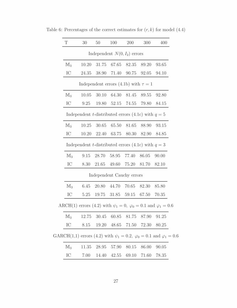
Table 6: Percentages of the correct estimates for (r, k) for model (4.4)

T 30 50 100 200 300 400

Independent N(0, I2) errors

M3 10.20 31.75 67.65 82.35 89.20 93.65

IC 24.35 38.90 71.40 90.75 92.05 94.10

Independent errors (4.1b) with τ = 1

M3 10.05 30.10 64.30 81.45 89.55 92.80

IC 9.25 19.80 52.15 74.55 79.80 84.15

Independent t-distributed errors (4.1c) with q = 5

M3 10.25 30.65 65.50 81.65 88.90 93.15

IC 10.20 22.40 63.75 80.30 82.90 84.85

Independent t-distributed errors (4.1c) with q = 3

M3 9.15 28.70 58.95 77.40 86.05 90.00

IC 8.30 21.65 49.60 75.20 81.70 82.10

Independent Cauchy errors

M3 6.45 20.80 44.70 70.65 82.30 85.80

IC 5.25 19.75 31.85 59.15 67.50 70.35

ARCH(1) errors (4.2) with ψ1 = 0, ϕ0 = 0.1 and ϕ1 = 0.6

M3 12.75 30.45 60.85 81.75 87.90 91.25

IC 8.15 19.20 48.65 71.50 72.30 80.25

GARCH(1,1) errors (4.2) with ψ1 = 0.2, ϕ0 = 0.1 and ϕ1 = 0.6

M3 11.35 28.95 57.90 80.15 86.00 90.05

IC 7.00 14.40 42.55 69.10 71.60 78.35

27

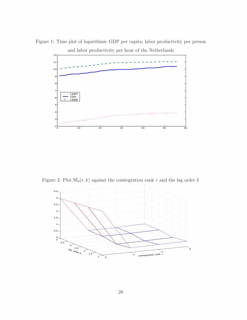
Figure 1: Time plot of logarithmic GDP per capita, labor productivity per person

and labor productivity per hour of the Netherlands

0 10 20 30 40 50 602

3

4

5

6

7

8

9

10

11

12

LpphGpcLppp

Figure 2: Plot M3(r, k) against the cointegration rank r and the lag order k

0 1

2 3

11.5

22.5

33.5

40

0.5

1

1.5

2

2.5

3

3.5

cointegration rank r

lag order k

28