On Discrete Location Choice Models

Nils Herger

Working Paper 13.02

This discussion paper series represents research work-in-progress and is distributed with the intention to foster discussion. The views herein solely represent those of the authors. No research paper in this series implies agreement by the Study Center Gerzensee and the Swiss National Bank, nor does it imply the policy views, nor potential policy of those institutions.

On Discrete Location Choice Models

February, 2013

Abstract

Within the context of the firm location choice problem, Guimaraes et al. (2003)have shown that a Poisson count regression and a conditional logit model yield identicalcoefficient estimates. Yet, the corresponding interpretation differs since these discretechoice models reflect polar cases as regards the degree with which the different loca-tions are similar. Schmidheiny and Brulhart (2011) have shown that these cases canbe reconciled by adding a fixed outside option to the choice set and transforming theconditional logit into a nested logit framework. This gives rise to a dissimilarity param-eter (λ) that equals 1 for the Poisson count regression (where locations are completelydissimilar) and 0 for the conditional logit model (where locations are completely sim-ilar). Though intermediate values are possible, the nested logit framework does notpermit the dissimilarity parameter to be pinned down. We show that, with panel dataand adopting a choice consistent normalisation, the fixed outside option can also beintroduced into the Poisson count framework, from which the estimation of the dissim-ilarity parameter is relatively straightforward. The different location choice models areillustrated with an empirical application using cross-border acquisitions data.

JEL classification: C25, F23Keywords: Conditional Logit Model, Location Choice, Nested Logit Model, Poisson

Count Regression

1

1 Introduction

Econometric models drawing on the discrete choices that are revealed when, for example,firms decide to locate in a given place, provide a popular framework to study the effect ofeconomic, political, or other factors on the geographical distribution of economic activities.Location choices can often be observed on a comprehensive basis since they manifest in suchthings as the establishment of new plants. For the case of foreign direct investment (FDI),for example, Devereux and Griffith (1998) uncover the extent to which corporate taxesinfluence the decision of US multinational enterprises (MNEs) to install local productioncapacity either in France, Germany, or the United Kingdom. Similarly, Buettner and Ruf(2007) analyse how corporate taxation affects the observed distribution of foreign plantsaffiliated to German multinationals, whilst Kim et al. (2003), Crozet et al. (2004), andDevereux et al. (2007) all study the role of agglomeration effects for FDI through the lensof individual location choices. All these studies account for the discrete nature of locationchoices by using an empirical framework of the binary or conditional logit class. Ratherthan contemplating the decisions of individual firms, a different strand of the literaturedraws on aggregated counts of such location choices. Considering again the example of FDI,Kessing et al. (2007), Herger et al. (2008), Hijzen et al. (2008), and Coeurdacier et al.(2009) all employ the number, or count, of cross-border acquisitions (CBAs) to uncover thedeterminants affecting the desire of MNEs to place economic activities in a given location.All these studies account for the discrete and non-negative nature of count data by employingregressions of the Poisson class.

The different approaches to analysing the empirical determinants to locate economic activi-ties raise the question of the econometric and economic differences between the conditionallogit approach with individual, and the Poisson count regression with aggregate locationchoices. Though these econometric models have been developed independently, they sharesome similarities. Specifically, for both cross-sectional and panel data, Guimaraes et al.(2003) have shown that the conditional logit model and Poisson count regression give rise toidentical coefficient estimates. This favours the usage of count data since the aggregation of,say, location choices entails a possibly dramatic reduction in the number of observations re-quired for estimation. However, according to Schmidheiny and Brulhart (2011)—henceforthSB—it is nevertheless important to distinguish between alternative location choice mod-els. In particular, though the coefficient estimates are identical, the results of the Poissoncount regression and conditional logit model differ when re-expressing the results in termsof elasticities. The reason is that in the Poisson count regression the aggregate number oflocation choices is used as the dependent variable, which can change with the value of theregressors. Borrowing the terminology of SB, the Poisson count regression reflects a ”posi-tive sum world”. Furthermore, when using count data, the locations are segmented in thesense that only the local conditions, but not those elsewhere, affect the dependent variable.Conversely, the conditional logit model reflects a ”zero sum world” since individual locationchoices are the dependent variable whilst their total number is exogenously fixed. This givesrise to spillover effects in the sense that an additional choice of a given location is alwaysoffset by an equivalent reduction elsewhere.

SB show that adding a fixed outside option gives rise to a nested logit model that encom-passes the polar cases embodied in the Poisson count regression and the conditional logitmodel. This may be intuitive since the main innovation of transforming the conditional logitinto a nested logit model is to summarise (location) choices into groups, or nests, that canbe more or less similar. The degree of segmentation between these groups manifests in theso-called dissimilarity parameter λ (sometimes also called the log-sum coefficient or inclusivevalue parameter). Within the context of location choices, SB show that the Poisson countregression implies that λ = 1, that is the elemental options are completely dissimilar, whilstthe conditional logit model arises when λ = 0, that is elemental options are entirely similar.

2

Yet, λ can in principle adopt any intermediate value on [0, 1]. Unfortunately, the nestedlogit framework of SB does not permit them to pin down the empirical value of λ.

This paper contributes to the literature by suggesting a way to extract the dissimilarityparameter from aggregated count data within a Poisson regression framework. One reasonwhy λ cannot be estimated in the SB framework is that their nested logit model is over-parameterised in terms of an overlap between the coefficient pertaining to the fixed outsideoption and the dissimilarity parameter that, hence, drops out of the likelihood function.It is well known that nested logit models suffer from an identification problem and, hence,require some suitable normalisation of the so-called scale parameters (Hunt, 2000; Ben Ak-tiva and Lerman, 1985; Hensher et al., 2005, ch.13). This step, which is arguably oftenignored in applied work, is crucial insofar as it gives rise to different versions of the nestedlogit model with different properties (Hunt, 2000; Hensher and Greene, 2005). Thereby, aminimal requirement would be that the normalisation is consistent with the basic principlesthat are thought to guide the (location) choices (Koppelman and Wen, 1998). For example,with a choice consistent normalisation, adding the same constant to all options should notchange the choice outcome. In this paper, we show that the normalisation of SB is notchoice consistent in this sense and propose an alternative normalisation to determine thedissimilarity parameter λ.

Based on a choice consistent normalisation, we then introduce the dissimilarity parameter λto the Poisson count framework using aggregate location choice data. From this, with paneldata, the dissimilarity parameter can be computed from the group effects of the Poissoncount regression without specific knowledge about the number of times the outside optionhas been chosen. Intuitively, the group effects of a Poisson count regression with panel dataabsorb the discrepancy between the observed number of location choices and the expectednumber from a basic Poisson process, and hence provide clues about the relative importanceof the (unobserved) outside option.

For several reasons, the value of the dissimilarity parameter can be important. Firstly,for a given sample, it indicates how far empirical location choices reflect a positive or zerosum world. Secondly, the dissimilarity parameter permits us to paint a more nuancedpicture when calculating the resulting elasticities by taking into account such things as(i.) differences of elasticities across locations (ii.) the magnitude of spillover effects whenthe economic or political conditions change elsewhere, or (iii.) the degree of similarity oflocations competing to attract a firm.

There are many applications where the differences between the various location choice mod-els could matter. We will apply these models to an example where location choices arerevealed in CBA deals within a sample of 25 EU countries. The reason is that this data iscomprehensively available and the location choices of MNEs lend themselves to the intro-duction of an outside option that could represent such contingencies as exporting to a givenmarket instead.

The paper is organised as follows. The first part reviews the contributions of Guimaraeset al. (2003) and SB that are relevant for the current context. In particular, to preparethe ground, section 2 discusses the similarities and differences between the basic conditionallogit model and Poisson count regression. Section 3 provides a synoptic overview of thenested logit model with a fixed outside option suggested by SB. Section 4 discusses the roleof choice consistent normalisations and, based on this, section 5 shows how the dissimilarityparameter λ can be computed within a Poisson count framework. Section 6 discusses theempirical application. Section 7 concludes.

3

2 Basic Location Choice Models

Consider the case where a firm wants to place some economic activities in a given location.Let the firms that are observed to undertake a location choice be indexed with i = 1, . . . , N .The domicile of the investing firms, or ”source” of the investment, is denoted with s =1, . . . , S whilst the choice set includes potential target locations, or ”hosts” of the investment,indexed with h = 1, . . . ,H. With profit maximising firms, the observed location choice—which is henceforth denoted by li,sh—reveals that the location h with profit opportunityE[Πi,sh] is expected to outperform all competing alternatives h′ that could in principle havebeen chosen instead. Hence,

li,sh =

{1 E[Πi,sh] > E[Πi,sh′ ] ∀ h 6= h′

0 otherwise.(1)

The conditional logit model employs location choices such as (1) as the dependent variable.Thereby, a set of choice-specific variables xsh is thought to impact upon profit expectationsE[Πi,sh] through the linear function

E[Πi,sh] = δs + x′shβ + εi,sh, (2)

where δs is a group effect absorbing source-specific factors. Furthermore, β denotes thecoefficients to be estimated. The component εi,sh accounts for stochastic factors that impactupon the location choice. To reflect that (1) uncovers the location with the highest expectedprofit opportunity, εi,sh is usually assumed to follow a Gumbel, or type 1 extreme valuedistribution (McFadden, 1974) where the location and scale parameter have been normalisedto, respectively, 0 and 1.1 The probability that a firm of s chooses h is then given by thecorresponding ratio between their expected number E[nsh] and the total number E[N ] =∑Ss=1

∑Hh=1E[nsh] of location choices within the sample, that is

Psh =exp

(x

′

shβ)∑S

s=1

∑Hh=1 exp

(x

′shβ) =

E[nclsh]

E[N ]. (3)

Owing to the logistic structure of (3), components such as δs that are fixed across thedifferent options drop out. Taking the joint distribution over all observed firms i, sources s,and host locations h yields the log likelihood function

lnLcl(β) =

S∑s=1

H∑h=1

nshPsh =

S∑s=1

{ H∑h=1

nshx′

shβ −H∑h=1

[nsh ln

H∑h=1

exp(x

′

shβ)]}

(4)

from which the coefficients β can be estimated. Guimaraes et al. (2003) show that a directregression onto the count variable nsh aggregating the number of location choices acrosssources and hosts provides an often more convenient way to estimate the coefficients β.This becomes clear when multiplying (3) with the denominator, which yields a conventional(panel) count regression with exponential mean transformation of

E[npcsh] = exp(δs + x′shβ

)= αsE[npcsh], (5)

where αs = ln(δs) and E[npcsh] = exp(x′shβ). Here, the group effect δs has been retained,but in principle the transformation between conditional logit and Poisson count regressionworks regardless of whether or not δs is included in (2). Assuming that the exponentialmean parameter E[npcsh] is Poisson distributed with probability density

1The Gumbel distribution, which is sometimes also referred to as type 1 extreme value distribution, hasa cumulative distribution function of F (`s, ςs) = exp(− exp(−(εi,sh − `s)/ςs)) where `s is the the so-calledlocation and ςs > 0 the scale parameter. For more details, see e.g. Ben-Akiva and Lerman (1985) or Hensheret al. (2005, ch.13 and 14).

4

P [npcsh] =exp(−E[npcsh])(E[npcsh])nsh

npcsh!(6)

yields coefficient estimates for β that are identical to those of the conditional logit model.To see why, contemplate the log likelihood contribution of s, that is

lnLpcs (αs, β) = −αsH∑h=1

exp(x′

shβ) + lnαs

H∑h=1

nsh +

H∑h=1

nshx′

shβ −H∑h=1

lnnsh! (7)

Setting the first derivative of this with respect to αs equal to 0, and solving for αs yields2

the maximum likelihood estimator of

αs =

∑Hh=1 nsh∑H

h=1 exp(x

′shβ) =

nsE[ns]

. (8)

Hence, for source s, αs absorbs the discrepancy between the observed number of aggre-gated location choices ns =

∑Hh=1 nsh and the corresponding expected number E[ns] =∑H

h=1 exp(xshβ) from the basic Poisson distribution. Thereby, 0 < αs < 1 and 1 < αsrepresent cases where, respectively, the number of observed location choices are ”underre-ported” and ”overreported” relative to the basic Poisson count distribution. Substituting (8)back into (7) and summing over all H hosts yields the concentrated log-likelihood function(that no longer depends on αs) given by

lnLpc(β) =

S∑s=1

{ H∑h=1

nshx′

shβ −H∑h=1

[nsh ln

H∑h=1

exp(x

′

shβ)]}

+ constant, (9)

which differs from (4) only as regards a constant with respect to β. Hence, the correspondingestimates are identical.

The variables xsh enter into the conditional logit model and the Poisson count regression in anon-linear manner. Hence, the coefficients β do not reflect a marginal effect (Hensher et al.,2005, pp.383ff.). This warrants the calculation of the elasticity η to reflect the percentagechange of the expected number E[nsh] of location choices between s and h in response toa percentage change of a given variable xsh,k. Though the same coefficients arise from theconditional logit model and the Poisson count regression, SB have recently drawn attentionto the differences in the resulting elasticities. Specifically, when expressing the variables inlogarithms, the own-elasticity of the Poisson count regression equals

ηpck =∂E[npcsh]

∂xsh,k

xsh,kE[npcsh]

= βk (10)

where βk denotes the coefficient pertaining to xsh,k and E[npcsh] is given by (5). Recall that inthe conditional logit model, individual location choices li,sh are the dependent variable. Thisimplies that the total number of location choices N is fixed—in the sense of not dependingon xsh—and the expected number of location choices between s and h is the probabilityweighted expression E[nclsh] = NPsh. Inserting (3) for Psh yields an elasticity of

ηclsh,k =∂E[nclsh]

∂xsh,k

xsh,kE[nsh]

= (1− Psh)βk. (11)

Owing to the properties of the probability Psh ∈ [0, 1], this is not larger than (10).

The different elasticities are a result of polar assumptions as regards the degree of similar-ity between different locations. In the Poisson count regression, the hosts are thought to

2A textbook discussion and derivation of the Poisson count regression with panel data can be found e.g.in Winkelmann (2008, ch.7.2) or Cameron and Trivedi (1998, ch.9).

5

represent alternatives that are dissimilar, or segmented, in the sense that a changing valueof the variable xsh,k affects the conditions in h, but not elsewhere in h′. The absence ofsuch spillovers manifests, statistically, in a cross-elasticity that is equal to zero by defini-tion.3 Borrowing the words of SB, this implies that the Poisson count regression reflects a”positive sum world” where e.g. improving conditions in h can result in an expansion of thetotal number of location choices N =

∑s

∑h nsh. Conversely, the conditional logit model

is a ”zero sum world” where the total number of location choices is fixed at N . When morefirms choose h, this comes entirely at the expense of competing alternatives within the setH of locations that are deemed to be similar.4

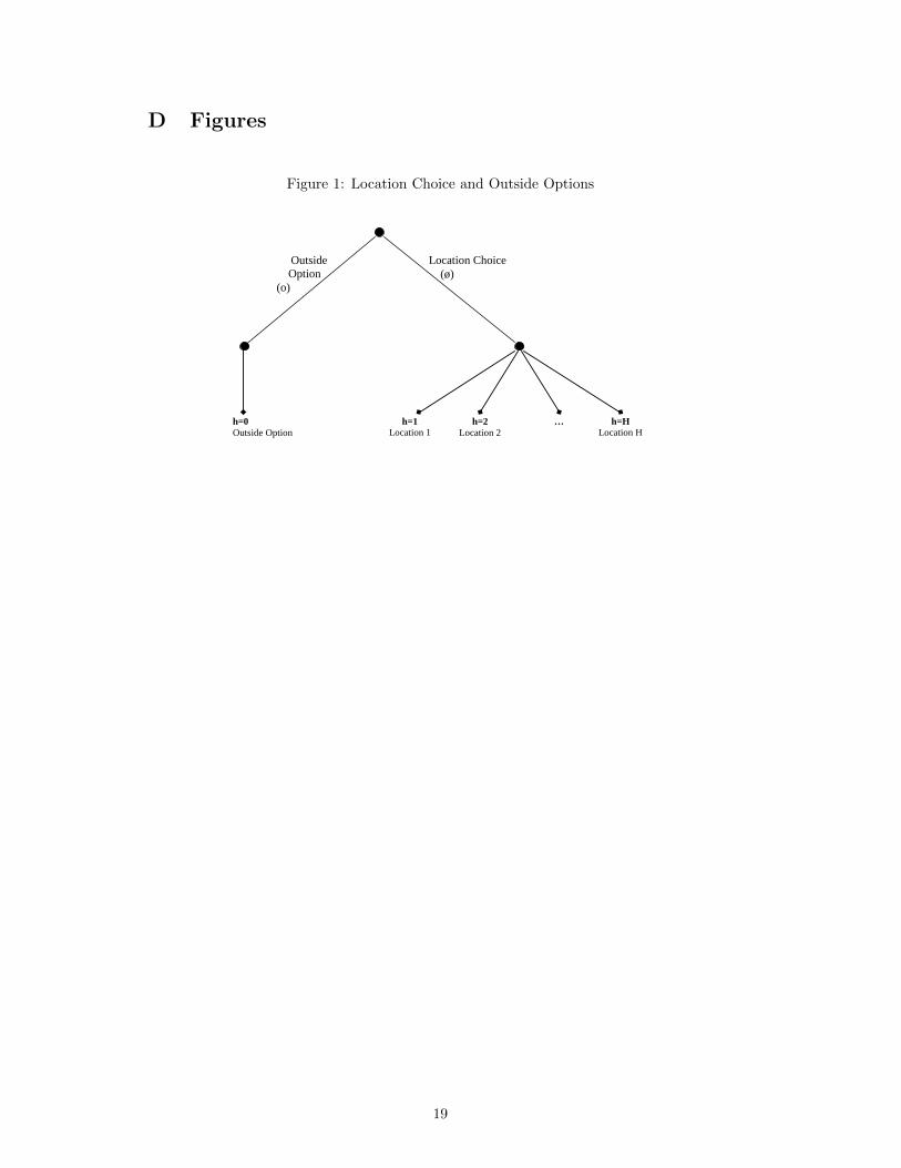
It is not always appropriate to restrict the alternative of locating in h to locating elsewhereas in the conditional logit model, or ignoring the role of alternatives altogether. Considerfor example the case of FDI. As depicted in a schematic manner in figure 1, a firm can eitherdecide to go multinational indexed with m = ø and, contingent on this, choose a host h tolocate a subsidiary plant. Alternatively, as depicted by the branch on the left, a firm canalso invest in a generic outside option m = o, which comprises only one elemental choice,labelled with h = 0, encompassing contingencies such as remaining inactive, exporting,installing capacity in the home country, etc.

FIGURE 1 HERE

Accounting explicitly for an outside option has other benefits. In particular, SB show thatthe extension of the conditional logit model with a fixed outside option yields a version ofthe nested logit model that covers the intermediate cases between the zero and positive-sumworld discussed above. The next section endeavours to develop this model within the currentcontext.

3 Location Choice in a Nested Logit Model

Following SB, and as depicted in figure 1, consider a scenario where the outside optionh = 0 is fixed in the sense of not depending on the choice-specific variables xsh. Hence, thecorresponding expected profit is given by

E[Πi,s0] = δs + εi,s0. (12)

Similar to (1), a firm is again assumed to pursue the outside option h = 0 if the resultingprofit is expected to outperform the alternative of placing economic activities in a givenlocation h > 0, with the corresponding decision being denoted by

mi,sh =

{0 E[Πi,s0] > E[Πi,sh] ∀ h > 01 otherwise.

(13)

The nested logit model entertains the idea that the elemental options can be summarised intodifferent groups consisting, here, of the outside option h = 0 and the location choice h > 0,whereby the elemental options are supposed to be more similar within than between thesedifferent ”nests”. To embed the approach of SB within the present context, the followingprovides a synoptic derivation of the choice probabilities of a nested logit model reflectingthe structure of figure 1.5

3Deriving (5) with respect to x′sh yields ζpcsh,k =∂E[n

pcsh

]

∂xsh′k

xsh′kE[n

pcsh

]= 0.

4Statistically, this manifests in a cross-elasticity of ζclsh,k = −Pshβk. Summing over all options H yields

(1−Psh)βk − (H − 1)Pshβk = (1−HPsh)βk = 0 and uncovers the zero-sum property in the sense that any”gain” of choices h is exactly offset by the ”losses” in the other options.

5For a textbook discussion of the nested logit model see Hensher et al. (2005, ch.13-14).

6

Consider first the basic location choice when a firm i does not want to pursue the outsideoption (where mi,sh = 1). Recall that the expected profits of (2) guiding the location choicehave a stochastic component to account for unobservable factors. However, in contrast tothe conditional logit model, εi,sh|ø conditions here on the firm not pursuing the outsideoption before making elemental decisions about the host h > 0. The stochastic componentεi,sh|ø is again assumed to be Gumbel-distributed with a location parameter normalised to0, but a variable scale parameter ςøs > 0 reflecting the similarity of the elemental optionswithin the group. Now, the conditional probability that a location h > 0 is chosen is givenby

Psh|ø =exp

(x

′

shβςøs

)∑Ss=1

∑Hh=1 exp

(x

′shβς

øs

) . (14)

This differs from (3) only with respect to the scale parameter ςøs , which was normalised to1 in the conditional logit model (see section 2). Turning to the group stage, the probabilityPøs that the outside option is not pursued depends again on a Gumbel distribution withscale parameter λø

s. From this, the probability Pøs is given by

Pøs =

[∑Ss=1

∑Hh=1 exp

(x

′

shβςøs

)]λøsςøs

[exp

(δsςos

)]λos+

[∑Ss=1

∑Hh=1 exp

(x

′shβς

øs

)]λøsςøs

, (15)

where the first term of the denominator accounts for the probability contribution of theoutside option (see below). The extent to which the options in the location choice groupdiffer manifests itself in the dissimilarity parameter6 (λø

s/ςøs ) ∈ [0, 1] which weights the

probability contribution of E[Nø] =∑Ss=1

∑Hh=1 exp(x′shβς

øs ) and is called ”inclusive value”

since it connects the elemental location choices of (14) with the group choice stage of (15).It can be shown that

(λøs/ς

øs ) =

√1− ρø

s (16)

where ρøs ∈ [0, 1] is the correlation between the stochastic components εi,sh|ø pertaining to the

profits from investing in different locations.7 Jointly, (14) and (15) define the unconditionalprobability of locating economic activities in h > 0, that is

Psh = Pøs × Psh|ø =

exp(x

′

shβςøs

)[∑Ss=1

∑Hh=1 exp

(x

′

shβςøs

)](λøsςøs−1)

[exp

(δsςos

)]λos+

[∑Ss=1

∑Hh=1 exp

(x

′shβς

øs

)]λøsςøs

. (17)

Consider now the fixed outside option o that represents a degenerated nest in the sense ofoffering only one basic ”choice” with h = 0. As discussed in Hunt (2000), in this case, thedistinction between unconditional and conditional probabilities is irrelevant, as Ps0|o = 1and Ps0 = Pos × Ps0|o. Since Pos = 1 − Pøs for the present binary choice with Pøs definedin (15), the probability of choosing the outside option is given by

Pos = Ps0 =exp

(δsς

os

)λos[exp

(δsςos

)]λos+

[∑Ss=1

∑Hh=1 exp

(x

′shβς

øs

)]λøsςøs

. (18)

6Sometimes this is also referred to as inclusive value parameter or log-sum coefficient.7A derivation of this result can be found in Hunt (2000, p.98).

7

The coefficients β can be estimated by means of maximum likelihood from the joint prob-abilities (17) and (18) across observed firms i. However, empirically, only the correlationρøs can be estimated from the data, but not the scale parameters λø

s and ςøs (Hunt, 2000;Ben-Aktiva and Lerman, 1985; Hensher et al., 2005, ch.13). In essence, this represents anover-identification problem that necessitates some normalisation. Usually, this involves set-ting some scale parameters at the group or basic choice level to 1 or 0. SB (p.217) set ςøs = 1,ςos = 1, and λos = 1 wherefore the probability of investing in the fixed outside option h = 0according to (17) or of choosing location h > 0 according to (18) becomes

Psh =

exp(x

′

shβ)[∑S

s=1

∑Hh=1 exp

(x

′

shβ)](λø

s−1)

exp(δs)

+

[∑Ss=1

∑Hh=1 exp

(x

′shβ)]λø

s=

exp(x′

shβ)(E[Nø])(λøs−1)

exp(δs) + (E[Nø])λøs

(19)

P0s =exp

(δs)

exp(δs)

+

[∑Ss=1

∑Hh=1 exp

(x

′shβ)]λø

s=

exp(δs)

exp(δs) + (E[Nø])λøs

(20)

where E[Nø] =∑Ss=1

∑Hh=1 exp(x

′

shβ) is the inclusive value when imposing the above men-tioned normalisation. Then, for firms domiciled in s, denoting the variable counting thenumber of times that the outside option has been chosen with nos and the number of timeswhere this is not the case with nøs, the concentrated log-likelihood function of the nestedlogit model with a fixed outside option, as derived in Appendix A.3 of SB, is given by

lnLnl(β) =

S∑s=1

{ H∑h=1

nshx′

shβ −H∑h=1

[nsh ln

H∑h=1

exp(x

′

shβ)]}

+ constant. (21)

Again, this differs from the Poisson count regression and the conditional logit model onlyup to a constant and hence yields identical estimates for the coefficients β. Furthermore,according to SB (2011, p.217), the elasticity of the nested logit model is given by

ηsh,k =∂E[nsh]

∂xsh,k= [1− Psh|ø(1− λø

sPs0)]βk, (22)

which coincides with the basic conditional logit model when λøs = 0 and with the basic

Poisson count regression when λøs = 1 and Ps0 = 1.

4 A Choice Consistent Normalisation

Though adding a fixed outside option leads to a location choice model encompassing thePoisson count and the conditional logit framework, the nested logit approach of section 3suffers from several drawbacks.

Firstly, the normalisation of the scale parameters λ and ς is a critical step in the sense ofleading to different versions of the nested logit model with different results and elasticities(Hunt, 2000; Hensher and Greene, 2005). Arguably, this aspect is often neglected in appliedwork (Louviere et al., 2000; Hensher et al., 2005, p.538). To avoid ambiguities, Koppelmanand Wen (1998) suggest that the normalisation should be consistent with some plausibleprinciples of choice theory. For example, since adding the same constant ∆ to all profitsof (2) and the outside option (12) would not change the ranking of the elemental options,a theoretically consistent nested logit model should be invariant to such a transformation.However, appendix A shows that the normalisation underlying (19) and (20) does not fulfillthis property.

Secondly, the scale parameter λs does not appear in the concentrated log likelihoodfunction (21) and, under the normalisation imposed in section 3, the maximum likelihoodestimate for δs and λs appear in the same first order condition

8

exp(δs) =nosnøs

[ H∑h=1

exp(x

′

shβ)]λs

(23)

and hence cannot be separately identified (SB, 2011, p.217).

We address these caveats by considering an alternative, choice consistent normalisation:

Proposition 1 Setting λos = λøs = λs, ς

øs = 1, and ςos = 0 represents a normalisation that

is consistent with choice theory in the sense that adding a constant ∆ to the profits (2) and(12) that guide the elemental choices does not change the choice outcome.

PROOF: Appendix A.

With the normalisation of proposition 1, the probability of opting for the outside optionaccording to (17), or of choosing location h > 0 according to (18) becomes

Psh =

exp(x

′

shβ)[∑S

s=1

∑Hh=1 exp

(x

′

shβ)](λs−1)

1 +

[∑Ss=1

∑Hh=1 exp

(x

′shβ)]λs =

(E[Nø])(λs−1)

1 + (E[Nf ])λsexp

(x

′

shβ)

(24)

Ps0 =1

1 +

[∑Ss=1

∑Hh=1 exp

(x

′shβ)]λs =

1

1 + (E[Nø])λs, (25)

Proposition 1 implies that exp(δsςos )λ

os = exp(0)λs = 1 and, hence, normalises to 1 the

contribution of the outside option.8 Intuitively, this is not problematic since the introductionof the scale parameter λs to the expected number of location choices E[Nø]λs , which appearsin the denominator of (24) and (25), already weights the relative importance between theoutside option and the location choices. Also, the normalisation of proposition 1 leaves thelikelihood function (21) intact since the parameter δs does not appear in it.

When ςøs = 1, according to (16), the scale parameter maps into the correlation between thestochastic component εi,sh of the elemental options, that is λs =

√1− ρs, and hence reflects

directly the degree of dissimilarity between the different locations. Recall that ρs = 0 meansthat stochastic events are entirely uncorrelated and the different locations are completelysegmented, which is consistent with the basic Poisson count regression with dissimilarityparameter λs = 1. Conversely, a dissimilarity parameter of λs = 0, which implies thatρs = 1, means that the locations are perfectly integrated, which is consistent with theconditional logit model.

Though with proposition 1, which implies that exp(δsςos )λ

os = exp(0)λs = 1, the dissimilarity

parameter λs could be estimated from (23), this would still necessitate information about thenumber of times nos that the outside option has been chosen. Considering again the exampleof FDI, this is not straightforward since contingencies such as abandoning an investmentproject or remaining inactive are hard to observe. However, the next section suggests thataggregating location choices provides a possible remedy, when the outside option is (partly)unobservable.

8A similar normalisation arises with the Logit model for binary choices where the probability of choosing

alternative 1 and 2 are, respectively, exp(x′β)/(1 + exp(x

′β)) and 1/(1 + exp(x

′β)) meaning that the weight

of one alternative has also been normalised to 1.

9

5 Introducing λs into the Poisson Count Framework

Similar to the basic models of section 2, the following endeavours to establish the linkbetween the nested logit model, where individual location choices are the dependent variable,and a corresponding Poisson count regression, where the aggregate number of such choicesis the dependent variable, when adding a fixed outside option to the choice set. Followingthe steps of section 2 to obtain a model with count variable nsh as dependent variable,multiplying the nested logit probability Psh of (24) with the expected total number of firmsE[N ] = 1 + (E[Nø])λs of the denominator yields

E[npcush ] = PshE[N ] = (E[Nø])(λs−1)︸ ︷︷ ︸=αs

exp(x

′

shβ)

= αsE[npcsh], (26)

which has a similar structure to (5), but the group effect that can be estimated from (8) hasbeen parameterised by αs = E[Nø](λs−1). When λs = 1, we have E[Nø](λs−1) = E[Nø]0 = 1and the basic Poisson count regression with completely dissimilar elemental options arises.Then, the inclusion of an outside option is irrelevant, which manifests itself in the fact thatE[npcush ] coincides with E[npcsh]. Conversely, when λs < 1, the elemental options are to somedegree similar and, the more this is the case, the more the expected number E[npcush ] oflocation choices differ from E[nsh] of a basic count process.

Solving αs = E[Nø](λs−1) for the dissimilarity parameter yields

λs =ln(E[Nø]αs)

ln(E[Nø]). (27)

Recall from the discussion in section 3 that λs can adopt values between 0 and 1. Then,λs = 1, which is consistent with the basic Poisson count regression, arises when αs = 1.Conversely, λs = 0, which is consistent with the basic conditional logit model, requiresthat αs = 1/E[Nø] which is close to 0 when a large number E[Nø] of location choicesare expected in the data. According to (8), when 0 < αs ≤ 1, the count data exhibitunderreporting in the sense that the observed number of location choices npcush is lowerthan would be expected from a basic Poisson count process with npcsh. Unless αs = 1,some firms will indeed end up choosing the (unobserved) outside option, which reduces thenumber of location choices actually observed. Hence, with aggregate counts, a high degree ofunderreporting can be interpreted as evidence of a higher importance of the outside option.Note that the establishment of this nexus between the nested logit model and the Poissoncount regression of (5) necessitates panel data to obtain the group effect (8) and computethe dissimilarity parameter λs in (27).

Finally, as derived in appendix B, the elasticity of npcush with respect to changes in xsh,k withcoefficient βk now equals

ηpcush,k = [1− Psh|ø(1− λs)]βk. (28)

This is again entirely consistent with the framework above in the sense that λs = 1 returnsthe elasticity of the basic Poisson count regression given by (10) and λs = 0 is the elasticityof the conditional logit model as given by (11). However, empirically, the dissimilarityparameter can adopt any value between these polar cases. Also, evaluating (28) yieldsηpcush,k = λsβk + (1−λs)(1−Psh|ø)βk = λsη

pcsh,k + (1−λs)ηclsh,k, meaning that the elasticity of

the Poisson count regression with a fixed outside option is a with λs weighted linear averagebetween the basic Poisson count regression and the conditional logit model. This reflectsa similar condition for the nested logit model that features in SB (2011,pp.217ff.). In sum,the introduction of an outside option leads to a more nuanced picture when calculatingthe resulting elasticities since the value of (28) depends on (i.) the coefficient βk whichdetermines the upper bound of the elasticity, (ii.) the probability Psh|ø that a host h can

10

attract a firm from elsewhere when changing the value of xsh,k, and (iii.) the extent towhich the locations are similar and hence compete to attract firms.

6 Empirical Application: Cross-Border Acquisitions

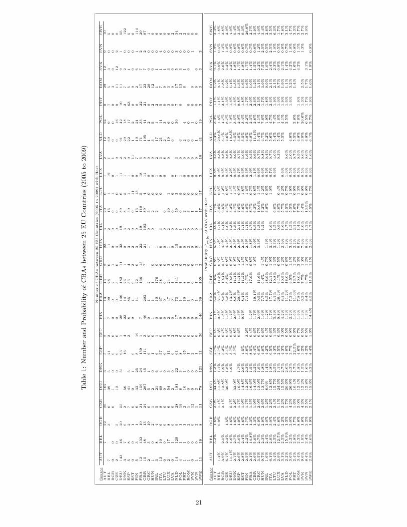
This section endeavours to illustrate the method from section 5 to calculate the dissimilarityparameter λs from the data with an application drawing on the location choices revealedwhen firms acquire a subsidiary plant abroad. Such CBAs are comprehensively recorded inthe SDC Platinum database of Thomson Reuters and have been used elsewhere to studythe determinants of FDI within the Poisson count framework (Kessing et al., 2007; Hergeret al., 2008; Hijzen et al., 2008; Coerdacier et al., 2009) and the conditional logit framework(Herger et al., 2011). To focus on a group, or nest, with relatively similar locations, theCBA deals between 25 EU countries during the 2005 to 2009 period are used. In total, thesample contains 8,302 deals with the top panel of Table 1 recording the count (number ofCBAs) between the source, reported in rows, and host, reported in columns.

TABLE 1 HERE

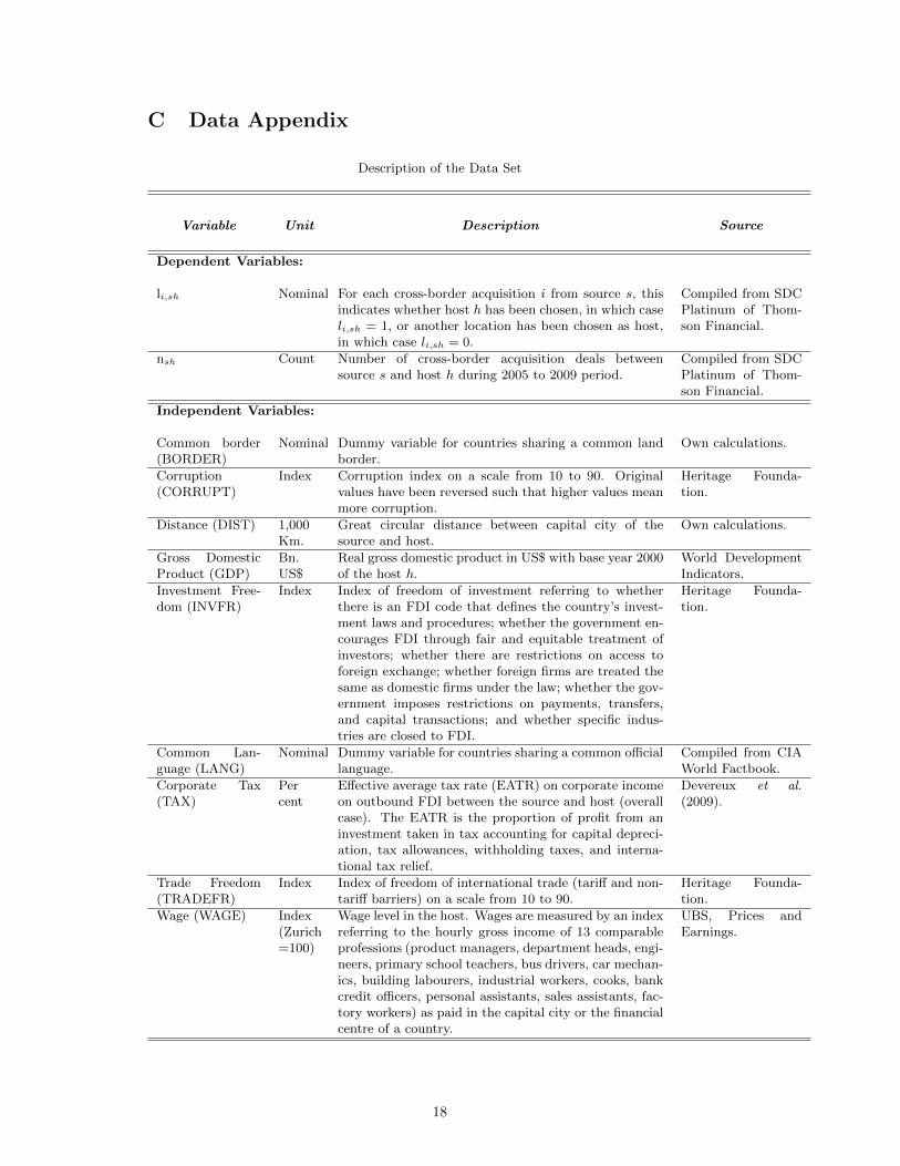
Following the literature on the determinants of FDI, the profit function (2) guiding the loca-tion choice is fitted to a gravity equation with the list of dependent variables x

′

sh containingreal GDP, the WAGE level, the distance (DIST) between the capital cities, a dummy variablefor countries sharing a common BORDER, a common language dummy variable (LANG),a measure for investment freedom (INVFR), an index on trade freedom (TRADEFR), acorruption index (CORRUPT), and a measure for the effective average taxes levied on cor-porations (TAX). Table 3 of appendix C contains a detailed description and the sources ofthe variables. Except for the dummy variables, the regressors have been transformed intologarithms and averaged over the 5 years under consideration. The resulting coefficients,calculated from a panel Poisson count regression with group effects αs and with the 600 (25source × 24 hosts) observations of nsh in the top panel of Table 1 as dependent variable,are given by

#CBAsh = αs ∗ exp

(0.74(0.02)

[0.02]

GDP − 1.04(0.06)

[0.06]

WAGE − 0.58(0.02)

[0.02]

DIST + 0.51(0.03)

[0.03]

BORDER+ 0.67(0.04)

[0.04]

LANG

+ 0.60(0.10)

[0.10]

INV FR− 3.89(0.87)

[0.88]

TRADEFR− 1.37(0.10)

[0.10]

CORRUPT − 0.40(0.10)

[0.10]

TAX

), (29)

whereby standard deviations are reported below the coefficients in (round) parentheses.Note that all coefficients are significant and shape up to the economic priors with more CBAsoccurring with economically large hosts that have low wages, are geographically close to thesource, have a common border or language, offer a high degree of investment freedom, aredifficult to access by trade, and have low levels of corruption and corporate taxes. Recallingthe discussion in section 2, a conditional logit model employing location choices li,sh revealedin individual CBA deals yields the same coefficient estimates. However, in practice, it is moreburdensome to handle such a location choice model since it involves 199,248 observations(24 possible choices × 8,302 deals) rather than the 600 when using aggregated count data.The standard deviations of the conditional logit model are reported in [square] brackets in(29) and barely differ, here, from those of the Poisson count process and do not overturnthe significance of any of the coefficient estimates. Conversely, since (7) contains a constantthat does not appear in (4), the value of the log likelihood function of the Poisson countregression, given by -2,139, is much less negative than the value of the conditional logitmodel given by -21,741.

The estimated group effects αs are reported in Table 2. Note that the values of αs are allbelow 1/3 which suggests that the number of observed CBA deals is substantially lower than

11

would be expected from a basic Poisson count regression without adjusting for the groupeffect of (8). The relatively low values of αs suggest that, within the current sample of EUcountries, firms often seem to favour the generic outside option.

TABLE 2 HERE

From the group effects αs of Table 2, the dissimilarity parameter λs can be computed from(27), whereby, from the estimates of (29), E[Nø] =

∑s

∑hE[nsh] =

∑s

∑h exp(x′shβ) =

132, 848. In general, for the current example, the values of the dissimilarity parameters arecloser to the bound with λs = 1 that reflects the ”positive sum world” of the Poisson countregression. This would suggest that additional CBAs with a given host country do often notcome at the expense of alternative locations. However, some differences arise between thecountries. What may be worth noting is that the dissimilarity parameter tends to be lowerfor the Eastern European countries that have only recently joined the EU. Perhaps, thesecountries have attracted a relatively large proportion of firms trying to outsource productionstages to low wage countries, which could be a type of investment that is subject to morerivalry between locations and is hence closer to the ”zero sum world” of the conditional logitmodel.

The value of the dissimilarity parameter also has implications for the calculation of elastic-ities. To see this, recall, from (10), that the coefficient estimates βk of (29) represent theupper bound of the absolute value of an elasticity ηpck reflecting the positive-sum world inher-ent in the Poisson count regression. Conversely, in the zero-sum world of the conditional logitmodel, which determines the lower bound ηclsh,k = (1−Psh)βk of (11), the elasticity dependsalso on the probability Psh that a firm domiciled in s invests in h. When the coefficient βk islow, such as the impact of taxation in (29) with an inelastic value of -0.40, or the probabilityPsh is modest, which is the case here for many country pairs as reported in the lower panelof Table 1, the range between these bounds is small. It may be intuitive that distinguishingbetween the zero and positive-sum world might be irrelevant when a variable is, statisticallyand economically, insignificant or a location is unlikely to attract a firm anyway, implyingthat changes of the local conditions have negligible spillover effects on to other locations.Conversely, when a variable has a potentially large impact, such as corruption which entersinto (29) with a coefficient of −1.39, and the probability of investment between s and h islarge, such as from Ireland into the UK where Psh = 0.49, the lower bound would e.g. beηclsh,k = (1 − 0.49)(−1.39) = −0.71 meaning about half the maximal value. Then, it mightbe important to pin down the position of the intermediate elasticity of (28). Consideringagain the case of corruption and using the range arising for a CBA from Ireland into the UK,with the relevant dissimilarity parameter being λs = 0.74 according to Table 2, applyingequation (28) yields an elasticity of ηpcush,k = 0.74× (−1.37) + (1− 0.74)× (−0.71) = −1.20.Hence, in this case, the elasticity would be closer to the upper bound.

Though the example presented in this section yields some intuitive results, our aim is merelyto illustrate how to calculate the dissimilarity parameter λs from the data with the methodfrom section 5. Of course, variables other than those in (29) have appeared in the literatureand considering them might affect the results. In any case, considering different locationchoice models and including the contingency of a fixed outside option leads to a more versatilepicture e.g. in terms of an elasticity whose value is not uniform across locations, but dependsalso on the conditions elsewhere or on the degree of similarity between competing locations.

7 Summary and Conclusion

Econometric models employing discrete location choices as the dependent variable havebecome a popular framework for uncovering how economic, political, and other determinantsaffect the geographical distribution of economic activities. Specifically, the econometric

12

analysis of location choices has taken the form of a conditional logit model, which connectsthe determinants with individual decisions to locate economic activities in a given place,or a Poisson regression aggregating such location choices into a count variable. Thoughthey yield identical coefficient estimates, the conditional logit model and the Poisson countregression reflect polar cases when it comes to the interpretation of the results. Aboveall, in the Poisson count regression, the locations are thought to be completely dissimilaroptions whilst in the conditional logit model they are completely similar. Previous work bySchmidheiny and Brulhart (2011) suggests that these polar cases can be reconciled by addinga fixed outside option and transforming the conditional into a nested logit model. This givesrise to a dissimilarity parameter λs whose value covers the continuum between the Poissoncount regression and the conditional logit model. However, outside options that cannot beobserved as well as data handling issues when there are a large number observations andlocations, can inhibit the empirical estimation of the dissimilarity parameter. For the caseof panel data, this paper has shown that the outside option can also be introduced into thePoisson count framework, where a group effect accounts for the underrecording of locationchoices and provides a way to uncover the value of the dissimilarity parameter. The mainadvantages of using such a Poisson count framework are that (1.) location choices takenfor example by firms are often easier to observe than, say, the value they invest and (2.)aggregating the location choices into a count variable can lead to a dramatic reduction inthe number of observations required for estimation.

13

References

Ben-Aktiva, M., and S.R. Lerman (1985), Discrete Choice Analysis: Theory and Applica-tion to Travel Demand, Cambridge: MIT Press.

Buettner, T. and M. Ruf (2007), Tax incentives and the location of FDI: evidence from apanel of German multinationals, International Tax and Public Finance 14: 151-164.

Cameron, C.A. and P.K. Trivedi (1998), Regression analysis of count data, Cambridge,Cambridge University Press.

Coerdacier, N., R. De Santis, and A. Aviat (2009), ’Cross-Border Mergers and Acquisitionsand European Integration’, Economic Policy, 55-106.

Crozet, M., T. Mayer, and J.L. Mucceilli (2004), How do firms agglomerate? A study ofFDI in France, Regional Science and Urban Economics 34: 27-54.

Devereux, M.P., C. Elschner, D. Enders, and C. Spengel (2009), ’Effective Tax Levels usingthe Devereux/Griffith Methodology’, Mannheim and Oxford: Centre for EuropeanEconomic Research.

Devereux, M. and R. Griffith (1998), Taxes and the location of production: evidence froma panel of US multinationals, Journal of Public Economics 68: 335-367.

Devereux, M., R. Griffith and H. Simpson (2007), Firm location decisions, regional grantsand agglomeration externalities, Journal of Public Economics 91: 413-435.

Guimaraes, P., O. Figueirdo and D. Woodward (2003), A Tractable Approach to the FirmLocation Decision Problem, The Review of Economics and Statistics 85: 201-204.

Hensher, D.A., J.M.Rose, and W.H.Greene (2005), Applied Choice Analysis, Cambridge:Cambridge University Press.

Hunt, G.L. (2002), Alternative nested logit model structures and the special case of partialdegeneracy, Journal of Regional Science 40: 89-113.

Herger, N., C. Kotsogiannis and S. McCorriston (2008), Cross-Border Acquisitions in theGlobal Food Sector, European Review of Agricultural Economics 35: 563-587.

Herger, N., C. Kotsogiannis and S. McCorriston (2008), International Taxation and FDIStrategies: Evidence from US Cross-Border Acquisitions, University of Exeter Eco-nomics Department Discussion Paper 11/09.

Hijzen, A., H. Gorg and M. Manchin (2008) Cross-border mergers & acquisitions and therole of trade costs, European Economic Review 52: 849-866.

Kessing, S., K.A. Konrad and C. Kotsogiannis (2007), Foreign direct investment and thedark side of decentralisation, Economic Policy 49, 5-70.

Kim, S.H., T.S. Pickton, and S. Gerking (2003), Foreign Direct Investment: AgglomerationEconomies and Returns to Promotion Expenditures, The Review of Regional Studies33: 61-72.

Koppelman, F.S., and C.H. Wen (1998), Alternative Nested Logit Models: Structure Prop-erties and Estimation, Transportation Research 32, 289-298.

Louviere, J.J., D.A. Hensher, and J.Swait (2000), Stated Choice Methods: Analysis andApplications in Marketing, Transportation and Environmental Evaluation, Cambridge:Cambridge University Press.

14

McFadden, D., (1974), Conditional logit analysis of qualitative choice behavior, In: Zarem-bka P. (Ed.) Frontiers in Econometrics. Academic Press, New York, 105-142.

Schmidheiny, K., and M. Brulhart (2011), On the equivalence of location choice models:Conditional logit, nested logit and Poisson, Journal of Urban Economics 69: 214-222.

UBS (various years), Prices and Earnings - A comparison of purchasing power around theglobe, Zurich.

Winkelmann, R. (2008), Econometric Analysis of Count Data, Berlin and Heidelberg:Springer (5th ed.).

15

A Proof Proposition 1

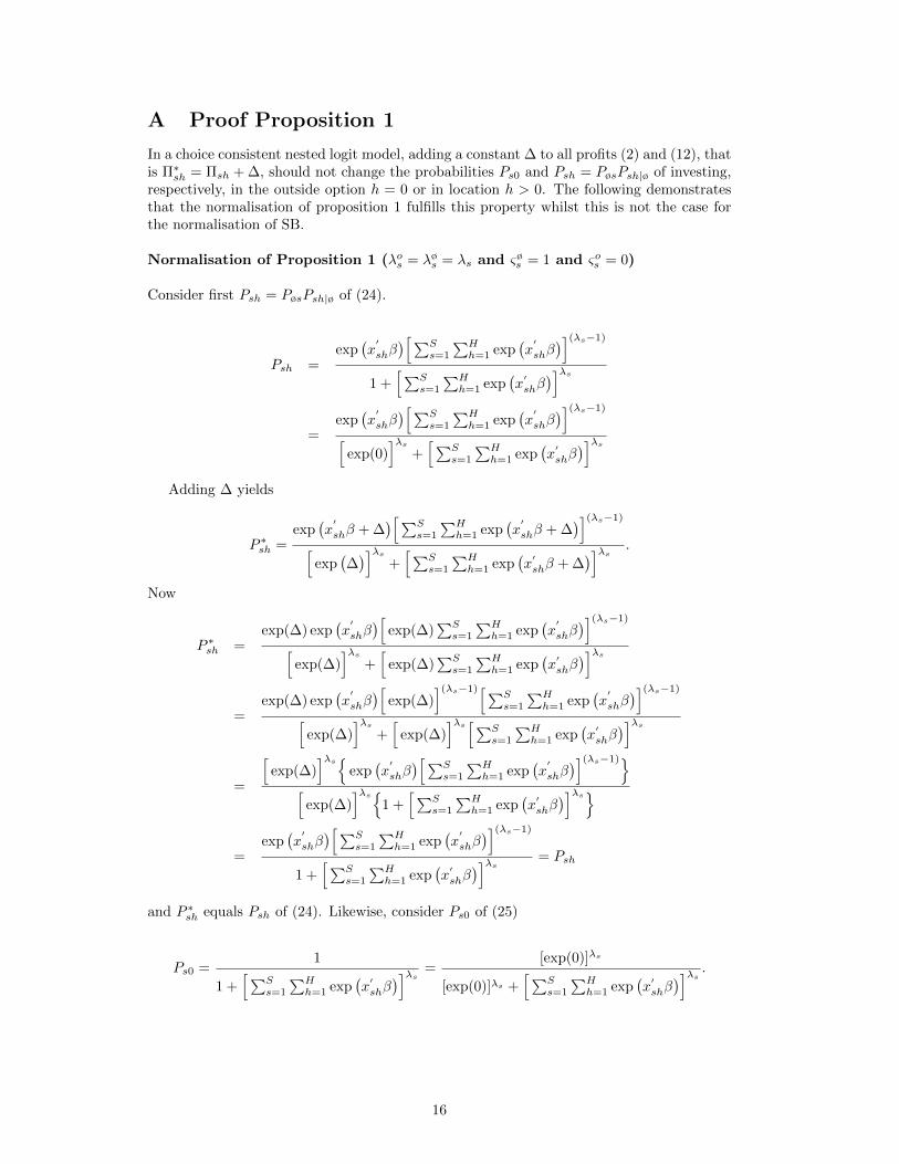
In a choice consistent nested logit model, adding a constant ∆ to all profits (2) and (12), thatis Π∗sh = Πsh + ∆, should not change the probabilities Ps0 and Psh = PøsPsh|ø of investing,respectively, in the outside option h = 0 or in location h > 0. The following demonstratesthat the normalisation of proposition 1 fulfills this property whilst this is not the case forthe normalisation of SB.

Normalisation of Proposition 1 (λos = λøs = λs and ςøs = 1 and ςos = 0)

Consider first Psh = PøsPsh|ø of (24).

Psh =exp

(x

′

shβ)[∑S

s=1

∑Hh=1 exp

(x

′

shβ)](λs−1)

1 +[∑S

s=1

∑Hh=1 exp

(x

′shβ)]λs

=exp

(x

′

shβ)[∑S

s=1

∑Hh=1 exp

(x

′

shβ)](λs−1)

[exp(0)

]λs+[∑S

s=1

∑Hh=1 exp

(x

′shβ)]λs

Adding ∆ yields

P ∗sh =exp

(x

′

shβ + ∆)[∑S

s=1

∑Hh=1 exp

(x

′

shβ + ∆)](λs−1)

[exp

(∆)]λs

+[∑S

s=1

∑Hh=1 exp

(x

′shβ + ∆

)]λs .

Now

P ∗sh =exp(∆) exp

(x

′

shβ)[

exp(∆)∑Ss=1

∑Hh=1 exp

(x

′

shβ)](λs−1)

[exp(∆)

]λs+[

exp(∆)∑Ss=1

∑Hh=1 exp

(x

′shβ)]λs

=exp(∆) exp

(x

′

shβ)[

exp(∆)](λs−1)[∑S

s=1

∑Hh=1 exp

(x

′

shβ)](λs−1)

[exp(∆)

]λs+[

exp(∆)]λs[∑S

s=1

∑Hh=1 exp

(x

′shβ)]λs

=

[exp(∆)

]λs{exp

(x

′

shβ)[∑S

s=1

∑Hh=1 exp

(x

′

shβ)](λs−1)}

[exp(∆)

]λs{1 +

[∑Ss=1

∑Hh=1 exp

(x

′shβ)]λs}

=exp

(x

′

shβ)[∑S

s=1

∑Hh=1 exp

(x

′

shβ)](λs−1)

1 +[∑S

s=1

∑Hh=1 exp

(x

′shβ)]λs = Psh

and P ∗sh equals Psh of (24). Likewise, consider Ps0 of (25)

Ps0 =1

1 +[∑S

s=1

∑Hh=1 exp

(x

′shβ)]λs =

[exp(0)]λs

[exp(0)]λs +[∑S

s=1

∑Hh=1 exp

(x

′shβ)]λs .

16

Adding ∆ yields

P ∗s0 =[exp(∆)]λs

[exp(∆)]λs +[∑S

s=1

∑Hh=1 exp

(x

′shβ + ∆

)]λs=

[exp(∆)]λs

[exp(∆)]λs +{[∑S

s=1

∑Hh=1 exp

(x

′shβ)]

exp(∆)}λs

=[exp(∆)]λs

[exp(∆)]λs + [exp(∆)]λs{[∑S

s=1

∑Hh=1 exp

(x

′shβ)]}λs

=1

1 +[∑S

s=1

∑Hh=1 exp

(x

′shβ)]λs = Ps0

which is equal to Ps0 of (25). Hence, the normalisation of Proposition 1 is choice consistent.

Schmidheiny and Bruhlhart Normalisation (ςøs = 1, ςos = 1, and λos = 1)

Adding ∆ to Ps0 of (20) yields

P ∗s0 =exp(δs + ∆)[

exp(δs + ∆

)]+[∑S

s=1

∑Hh=1 exp

(x

′shβ + ∆

)]λøs.

and

P ∗s0 =exp(δs) exp(∆)

exp(δs) exp(∆) +{[∑S

s=1

∑Hh=1 exp

(x

′shβ)]

exp(∆)}λø

s

=exp(δs) exp(∆)

exp(δs) exp(∆) + exp(∆)λøs

[(∑Ss=1

∑Hh=1 exp(x

′shβ)

)]λøs6= Ps0

Hence the normalisation of SB is choice inconsistent.

B Derivation of Elasticity

With E[npcush ] = (E[Nø])(λs−1) exp(x′

shβ) of (26), the elasticity with respect to a (logarith-mically transformed) variable xsh,k is

ηpcush =∂E[npcush ]

∂xsh,k

xsh,k

E[npcush ]

=

[(λs − 1)(E[Nø])(λs−2) exp(.)

βk

xsh,kexp(.) + E[Nø](λs−1) exp(.)

βk

xsh,k

]xsh,k

E[Nø](λs−1) exp(.).

Cancelling terms yields

ηpcush = (λs − 1) (E[Nø])−1 exp(x′

shβ)︸ ︷︷ ︸=Psh|ø according to (14)

βk + βk

= [1 + (λs − 1)Psh|ø]βk = [1− (1− λs)Psh|ø]βk.

17

C Data Appendix

Description of the Data Set

Variable Unit Description Source

Dependent Variables:

li,sh Nominal For each cross-border acquisition i from source s, thisindicates whether host h has been chosen, in which caseli,sh = 1, or another location has been chosen as host,in which case li,sh = 0.

Compiled from SDCPlatinum of Thom-son Financial.

nsh Count Number of cross-border acquisition deals betweensource s and host h during 2005 to 2009 period.

Compiled from SDCPlatinum of Thom-son Financial.

Independent Variables:

Common border(BORDER)

Nominal Dummy variable for countries sharing a common landborder.

Own calculations.

Corruption(CORRUPT)

Index Corruption index on a scale from 10 to 90. Originalvalues have been reversed such that higher values meanmore corruption.

Heritage Founda-tion.

Distance (DIST) 1,000Km.

Great circular distance between capital city of thesource and host.

Own calculations.

Gross DomesticProduct (GDP)

Bn.US$

Real gross domestic product in US$ with base year 2000of the host h.

World DevelopmentIndicators.

Investment Free-dom (INVFR)

Index Index of freedom of investment referring to whetherthere is an FDI code that defines the country’s invest-ment laws and procedures; whether the government en-courages FDI through fair and equitable treatment ofinvestors; whether there are restrictions on access toforeign exchange; whether foreign firms are treated thesame as domestic firms under the law; whether the gov-ernment imposes restrictions on payments, transfers,and capital transactions; and whether specific indus-tries are closed to FDI.

Heritage Founda-tion.

Common Lan-guage (LANG)

Nominal Dummy variable for countries sharing a common officiallanguage.

Compiled from CIAWorld Factbook.

Corporate Tax(TAX)

Percent

Effective average tax rate (EATR) on corporate incomeon outbound FDI between the source and host (overallcase). The EATR is the proportion of profit from aninvestment taken in tax accounting for capital depreci-ation, tax allowances, withholding taxes, and interna-tional tax relief.

Devereux et al.(2009).

Trade Freedom(TRADEFR)

Index Index of freedom of international trade (tariff and non-tariff barriers) on a scale from 10 to 90.

Heritage Founda-tion.

Wage (WAGE) Index(Zurich=100)

Wage level in the host. Wages are measured by an indexreferring to the hourly gross income of 13 comparableprofessions (product managers, department heads, engi-neers, primary school teachers, bus drivers, car mechan-ics, building labourers, industrial workers, cooks, bankcredit officers, personal assistants, sales assistants, fac-tory workers) as paid in the capital city or the financialcentre of a country.

UBS, Prices andEarnings.

18

D Figures

Figure 1: Location Choice and Outside Options

Location Choice (ø)

Outside

Option (o)

h=0 Outside Option

h=1 Location 1

h=2 Location 2

h=H Location H

…

19

E Tables

20

Tab

le1:

Nu

mb

eran

dP

rob

ab

ilit

yof

CB

As

bet

wee

n25

EU

Cou

ntr

ies

(2005

to2009)

Num

ber

of

CB

As

betw

een

25

EU

Countrie

s(2005

to

2009)

wit

hH

ost

Source

AU

TB

EL

BG

RC

ZE

DE

UD

NK

ESP

EST

FIN

FR

AG

BR

GR

CH

UN

IRL

ITA

LT

UL

UX

LV

AN

LD

PO

LP

RT

RO

MSV

KSV

NSW

EA

UT

722

26

162

35

21

13

13

223

320

01

212

24

029

12

910

BE

L7

36

39

521

37

99

28

011

216

112

169

97

53

05

BG

R0

00

10

00

00

21

00

01

01

00

03

00

0C

ZE

20

512

00

00

03

04

00

01

00

16

011

12

20

DE

U143

46

20

55

51

63

128

146

182

11

33

19

89

611

291

42

10

11

91

55

DN

K3

70

356

16

423

14

26

10

38

51

220

18

27

20

122

ESP

58

27

41

53

885

53

43

250

11

022

17

63

51

05

EST

00

10

01

09

10

32

00

11

011

12

00

00

0F

IN5

31

632

25

819

11

22

03

013

13

07

10

21

02

61

114

FR

A13

133

10

31

159

24

139

17

166

15

22

19

110

518

671

35

22

17

72

29

GB

R15

48

13

24

287

45

111

340

202

721

102

89

411

0105

41

21

23

72

97

GR

C2

319

05

16

00

12

10

50

00

12

020

00

1H

UN

10

21

20

10

11

10

02

00

03

52

12

00

0IR

L3

84

521

66

10

10

176

01

20

12

17

12

11

06

ITA

13

10

68

68

457

06

67

58

68

30

93

21

11

57

14

6LT

U0

00

00

00

50

00

00

00

08

23

00

10

0L

UX

217

86

54

311

42

47

24

31

240

10

19

63

33

06

LV

A0

10

02

00

20

01

00

00

60

00

00

00

2N

LD

14

129

928

181

22

61

217

73

141

215

959

37

330

717

53

34

PO

L4

11

19

83

80

01

10

61

09

10

60

13

30

2P

RT

11

12

10

145

00

10

82

02

20

00

24

61

02

RO

M1

02

10

01

00

11

02

03

00

00

00

00

0SV

K0

00

12

00

20

00

00

00

10

00

01

00

10

SV

N1

02

12

01

00

11

10

01

00

01

00

00

0SW

E11

18

811

78

121

31

20

140

38

105

21

417

17

310

41

19

33

33

Probabilit

yPsh|ø

of

CB

Aw

ith

Host

Source

AU

TB

EL

BG

RC

ZE

DE

UD

NK

ESP

EST

FIN

FR

AG

BR

GR

CH

UN

IRL

ITA

LT

UL

UX

LV

AN

LD

PO

LP

RT

RO

MSV

KSV

NSW

EA

UT

3.3

%1.6

%3.9

%34.4

%1.3

%2.7

%0.4

%1.1

%5.5

%6.6

%0.8

%5.8

%0.9

%7.7

%0.7

%0.8

%0.5

%3.4

%3.0

%1.1

%1.2

%9.1

%1.9

%2.3

%B

EL

1.4

%0.9

%1.1

%11.8

%1.1

%2.7

%0.3

%0.8

%31.5

%11.8

%0.5

%1.2

%1.1

%3.0

%0.4

%2.9

%0.3

%20.6

%1.6

%1.1

%0.7

%0.9

%0.5

%1.8

%B

GR

3.9

%2.5

%2.1

%12.8

%1.9

%5.2

%0.7

%1.8

%8.8

%10.4

%5.1

%4.0

%1.4

%9.5

%1.2

%0.6

%0.8

%5.1

%4.7

%2.1

%7.8

%2.6

%1.3

%3.8

%C

ZE

6.7

%2.2

%1.5

%30.9

%1.8

%3.1

%0.5

%1.3

%6.8

%8.4

%0.8

%4.4

%1.0

%4.7

%0.8

%0.5

%0.6

%4.6

%8.7

%1.3

%1.2

%4.2

%1.0

%2.9

%D

EU

11.1

%4.6

%1.6

%5.7

%4.9

%3.7

%0.6

%1.7

%13.7

%10.8

%0.9

%2.6

%1.3

%5.2

%1.1

%2.2

%0.8

%10.3

%7.0

%1.6

%1.4

%2.2

%0.9

%4.0

%D

NK

2.7

%2.7

%1.6

%2.2

%32.0

%3.7

%0.8

%2.0

%8.0

%11.4

%0.9

%2.3

%1.5

%4.7

%1.1

%0.6

%0.9

%6.5

%3.5

%1.6

%1.3

%1.8

%0.8

%5.4

%E

SP

2.6

%3.0

%1.9

%1.7

%10.9

%1.7

%0.6

%1.5

%20.5

%14.4

%1.2

%2.3

%2.1

%7.6

%0.9

%0.7

%0.7

%5.8

%2.9

%9.8

%1.5

%1.7

%0.9

%3.3

%E

ST

2.8

%2.4

%1.6

%1.9

%14.8

%2.6

%4.5

%9.7

%8.4

%11.2

%1.1

%2.4

%1.4

%5.6

%1.8

%0.6

%3.0

%5.5

%3.4

%1.8

%1.6

%1.8

%0.8

%9.3

%F

IN2.5

%2.2

%1.7

%1.7

%12.2

%2.3

%3.8

%3.2

%7.1

%9.7

%1.0

%2.3

%1.4

%4.8

%1.6

%0.5

%1.6

%4.8

%3.2

%1.7

%1.6

%1.7

%0.7

%26.8

%F

RA

2.1

%14.8

%1.3

%1.5

%16.6

%1.5

%8.5

%0.4

%1.2

%17.9

%0.8

%1.8

%1.7

%8.7

%0.7

%2.9

%0.5

%6.8

%2.3

%2.0

%1.0

%1.4

%0.7

%2.7

%G

BR

2.6

%5.9

%1.3

%1.9

%14.0

%2.2

%6.4

%0.6

%1.7

%19.1

%1.0

%2.0

%8.5

%6.3

%0.8

%1.1

%0.6

%11.4

%2.8

%2.6

%1.2

%1.5

%0.8

%3.9

%G

RC

3.5

%2.7

%6.9

%2.0

%13.0

%1.9

%6.0

%0.7

%2.0

%9.5

%11.6

%3.3

%1.3

%10.6

%1.1

%0.6

%0.7

%5.4

%4.1

%2.5

%3.1

%2.2

%1.2

%4.0

%H

UN

9.7

%2.3

%2.9

%2.6

%13.7

%1.8

%4.0

%0.6

%1.6

%7.7

%9.4

%1.4

%1.2

%7.2

%1.2

%0.6

%0.8

%4.7

%7.6

%1.7

%3.9

%7.5

%2.5

%3.4

%IR

L1.6

%2.4

%1.0

%1.2

%8.0

%1.4

%4.2

%0.4

%1.2

%8.5

%48.9

%0.7

%1.3

%3.8

%0.6

%0.5

%0.4

%5.2

%1.9

%1.8

%0.9

%1.0

%0.5

%2.6

%IT

A6.1

%2.9

%3.0

%2.2

%12.8

%1.8

%6.5

%0.6

%1.7

%17.7

%12.1

%1.9

%3.4

%1.6

%1.0

%0.7

%0.7

%5.6

%4.7

%2.6

%2.1

%2.4

%2.5

%3.5

%LT

U3.4

%2.5

%2.4

%2.4

%15.7

%2.5

%4.3

%1.3

%3.3

%8.1

%10.8

%1.3

%3.3

%1.5

%6.0

%0.6

%4.0

%5.4

%7.4

%1.9

%2.1

%2.3

%1.0

%6.3

%L

UX

2.9

%12.5

%0.8

%1.1

%24.3

%1.1

%2.5

%0.3

%0.8

%26.4

%9.1

%0.5

%1.2

%0.9

%3.0

%0.4

%0.3

%5.4

%1.6

%1.0

%0.7

%0.9

%0.5

%1.7

%LV

A3.1

%2.5

%2.2

%2.2

%15.5

%2.7

%4.3

%3.0

%4.2

%8.1

%10.9

%1.2

%2.9

%1.6

%5.7

%5.2

%0.6

%5.5

%4.1

%1.9

%1.9

%2.1

%0.9

%7.8

%N

LD

2.2

%15.9

%1.3

%1.7

%20.6

%2.0

%4.0

%0.5

%1.3

%11.2

%18.0

%0.8

%1.8

%1.7

%4.5

%0.7

%1.0

%0.6

%2.5

%1.6

%1.1

%1.4

%0.7

%3.1

%P

OL

3.6

%2.2

%2.0

%4.2

%26.9

%2.3

%3.7

%0.9

%2.2

%7.3

%9.5

%1.1

%3.3

%1.2

%5.5

%1.9

%0.5

%2.0

%4.9

%1.6

%3.2

%4.2

%1.0

%4.7

%P

RT

2.4

%2.8

%1.7

%1.6

%10.4

%1.7

%22.5

%0.6

%1.6

%11.0

%13.7

%1.2

%2.2

%2.1

%7.0

%0.9

%0.6

%0.7

%5.5

%2.8

%1.4

%1.6

%0.8

%3.3

%R

OM

3.4

%2.3

%8.8

%2.0

%12.4

%1.8

%4.6

%0.7

%1.9

%7.8

%10.0

%2.3

%6.7

%1.4

%7.7

%1.3

%0.5

%0.9

%4.8

%7.6

%1.9

%4.2

%1.1

%3.7

%SV

K9.6

%1.9

%1.8

%4.3

%12.2

%1.5

%3.2

%0.5

%1.3

%6.3

%7.7

%1.0

%7.9

%1.0

%5.4

%0.9

%0.5

%0.6

%3.9

%20.6

%1.3

%2.5

%1.3

%2.7

%SV

N8.4

%2.4

%2.2

%2.5

%12.8

%1.6

%4.2

%0.5

%1.4

%8.4

%9.7

%1.2

%6.4

%1.2

%13.9

%0.9

%0.6

%0.6

%4.8

%6.5

%1.7

%1.7

%3.1

%3.0

%SW

E2.9

%2.6

%1.9

%2.1

%15.6

%3.2

%4.4

%1.6

%14.4

%8.5

%11.9

%1.1

%2.6

%1.7

%5.5

%1.7

%0.6

%1.6

%6.1

%3.7

%1.9

%1.6

%1.9

%0.9

%

21

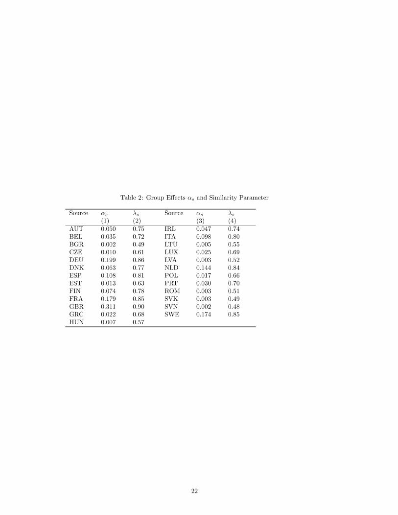
Table 2: Group Effects αs and Similarity Parameter

Source αs λs Source αs λs(1) (2) (3) (4)

AUT 0.050 0.75 IRL 0.047 0.74BEL 0.035 0.72 ITA 0.098 0.80BGR 0.002 0.49 LTU 0.005 0.55CZE 0.010 0.61 LUX 0.025 0.69DEU 0.199 0.86 LVA 0.003 0.52DNK 0.063 0.77 NLD 0.144 0.84ESP 0.108 0.81 POL 0.017 0.66EST 0.013 0.63 PRT 0.030 0.70FIN 0.074 0.78 ROM 0.003 0.51FRA 0.179 0.85 SVK 0.003 0.49GBR 0.311 0.90 SVN 0.002 0.48GRC 0.022 0.68 SWE 0.174 0.85HUN 0.007 0.57

22