On Forced Temperature Changes, Internal … Forced Temperature Changes, Internal Variability and the AMO Michael E. Mann Byron A. Steinman Sonya K. Miller Department of Meteorology

©2014 American Geophysical Union. All rights reserved.

On Forced Temperature Changes, Internal Variability and the AMO

Michael E. Mann

Byron A. Steinman

Sonya K. Miller

Department of Meteorology and Earth and Environmental Systems Institute,

Pennsylvania State University, University Park, PA, USA 16802

Geophysical Research Letters (revised Mar 12, 2014)

This article has been accepted for publication and undergone full peer review but has not been through the copyediting, typesetting, pagination and proofreading process which may lead to differences between this version and the Version of Record. Please cite this article as doi: 10.1002/2014GL059233


Abstract

We estimate the low-frequency internal variability of Northern Hemisphere (NH)

mean temperature using observed temperature variations, which include both forced

and internal variability components, and several alternative model simulations of the

(natural + anthropogenic) forced component alone. We then generate an ensemble of

alternative historical temperature histories based on the statistics of the estimated

internal variability. Using this ensemble, we show, firstly, that recent NH mean

temperatures fall within the range of expected multidecadal variability. Using the

synthetic temperature histories, we also show that certain procedures used in past

studies to estimate internal variability, and in particular, an internal multidecadal

oscillation termed the “Atlantic Multidecadal Oscillation” or “AMO”, fail to isolate

the true internal variability when it is a priori known. Such procedures yield an AMO

signal with an inflated amplitude and biased phase, attributing some of the recent NH

mean temperature rise to the AMO. The true AMO signal, instead, appears likely to

have been in a cooling phase in recent decades, offsetting some of the anthropogenic

warming. Claims of multidecadal “stadium wave” patterns of variation across

multiple climate indices are also shown to likely be an artifact of this flawed

procedure for isolating putative climate oscillations.

Keywords: AMO, climate oscillations, internal/forced variability, stadium waves

Index Terms: 1616, 3305, 4215


1. Introduction

Evidence for a multidecadal climate oscillation centered in the North Atlantic

originated in work by Folland and colleagues during the 1980s [Folland et al 1984;

1986]. Additional support was provided in subsequent analyses of observational

climate data [e.g. Kushnir et al, 1994]. The confident establishment of any low-

frequency oscillatory climate signal, however, was hampered by the limited (roughly

one century) length of the instrumental climate record and the potential contamination

of putative low-frequency oscillations by forced long-term climate trends. Subsequent

work in the mid-1990s attempted to address these limitations. Mann and Park

[1994;1996] used a multivariate signal detection approach to separate distinct long-

term climate signals, while Schlesinger and Ramankutty [1994] employed climate

model simulations to estimate and remove the forced trend from observations. These

analyses provided further evidence for a multidecadal (50-70 year) timescale signal

centered in the North Atlantic with a weak projection onto hemispheric mean

temperature. Mann et al [1995] presented evidence based on the analyses of

paleoclimate proxy data that such a signal persists several centuries back in time.

Meanwhile, climate model simulations by Delworth et al [1993; 1997] demonstrated

the existence of an internal multidecadal oscillation associated with the North Atlantic

meridional overturning circulation (“AMOC”) and coupled ocean-atmosphere

processes in the North Atlantic. Delworth and Mann [2000] provided consistent

evidence across instrumental observations, paleoclimate data, and coupled model

simulations, for the existence of a distinct multidecadal climate mode. This mode was

subsequently termed the “Atlantic Multidecadal Oscillation” (“AMO”) in Kerr [2000]


[the term was coined by M. Mann in an interview with Kerr—see Mann, 2012]. In

this article, we reserve the term AMO to denote such an internal, multidecadal

timescale oscillation.

In most studies, the AMO surface temperature signal is found to be concentrated in

the high latitudes of the North Atlantic, while the projection onto Northern

Hemisphere (NH) mean temperature is modest. Knight et al [2005] demonstrated the

existence of an AMO signal in a 1400 year control simulation of the Hadley Centre

(HadCM3) coupled model with peak temperature variations approaching 0.5 oC in the

high latitudes of the North Atlantic, but with an NH mean amplitude of only ~0.1oC.

The signal in the tropical North Atlantic was also found to be only ~0.1oC in peak

amplitude.

Some analyses have argued for a substantially larger expression of the AMO in NH

mean temperature and/or tropical Atlantic temperatures [e.g. Enfield et al, 2001;

Goldenberg et al, 2001; Wyatt et al 2012; Wyatt and Curry, 2013]. These studies

employed what we will henceforth refer to as the “Detrended-AMO” approach: the

AMO signal was defined as the low-frequency component that remains after linearly

detrending surface temperatures. Other studies, however, have demonstrated likely

artifacts of that procedure [Trenberth and Shea, 2006; Mann and Emanuel, 2006;

Delworth et al, 2007; Ting et al, 2009]. For example, Mann and Emanuel [2006]

show that such a procedure misattributes at least part of the forced cooling of the NH

by anthropogenic aerosols during the 1950s-1970s (especially over parts of the North

Atlantic) to the purported down-swing of an internal “AMO” oscillation. A number of

climate modeling studies support their finding [Santer et al, 2006; Booth et al, 2012;


Evan, 2012; Dunstone et al, 2013], though the precise role that anthropogenic

aerosols have played in recent decades continues to be debated in the literature [Koch

et al, 2011; Carslaw et al, 2013; Stevens, 2013].

In this study, we take a different approach to diagnosing the expression of the AMO.

Noting that previous studies have established that the AMO, while centered in the

North Atlantic, projects onto Northern Hemisphere mean temperature, we focus

specifically on its hemispheric projection. This eliminates the need for more complex

spatiotemporal signal detection approaches [e.g. Mann and Park, 1994; Delworth and

Mann, 2000], though it precludes drawing inferences about the regional AMO

footprint. Like Schlesinger and Ramankutty [1994], we use model estimates of the

forced trend in NH mean temperature. We account, however, for key natural (solar

and volcanic) radiative forcings not included in that former study. Moreover, we use

the procedure to assess the potential bias of certain approaches for detecting and

defining an AMO signal. Estimating the internal variability (“AMO”) component by

differencing the observed and estimated forced historical NH temperature variations

(henceforth the “Differenced-AMO” approach), we construct a simple statistical

model for the internal variability. We then produce a set of alternative internal

variability realizations and, accordingly, an ensemble of plausible synthetic NH mean

temperature histories.

Using this ensemble, we firstly investigate the issue [e.g. The Economist, 2013; Allen

et al, 2013] of whether temperature changes over the past decade fall within the range

of expected low-frequency natural variability. Then by knowing the true “AMO”

signal for each of the synthetic temperature histories, we are able to test the ability of


the Detrended-AMO approach to recover that signal. Finally, we examine the related

“stadium wave” hypothesis of Wyatt and collaborators [Wyatt et al 2012; Wyatt and

Curry, 2013], wherein a series of climate indices are analyzed for AMO behavior via

the Detrended-AMO approach, and are interpreted as providing evidence for a

coherent multidecadal oscillation propagating through the global climate system.

2. Methods

We employed a simple zero-dimensional Energy Balance Model (“EBM” —see e.g.

North et al [1981]) of the form:

C dT/dt = S(1-)/4 + FRAD -A-BT

to estimate the forced response of the Northern Hemisphere mean temperature to

natural (volcanic and solar) and anthropogenic (well-mixed greenhouse gases and

Northern Hemisphere mean tropospheric aerosol) radiative forcing [see Mann 2011;

Mann et al 2012].

T is the temperature of Earth’s surface (approximated at the surface of a 70 m depth

mixed layer ocean covering 70% of Earth’s surface area). C=2.08 x 108 J K

-1m

-2 is an

effective heat capacity that accounts for the thermal inertia of the mixed layer ocean.

S ≈1370 Wm-2

is the “solar constant” and =0.3 is the effective surface albedo. The

linear “gray body” approximation LW=A+BT was used to model outgoing long-wave

radiation, where the choice of B dictates the equilibrium climate sensitivity

(ECS)T2xCO2. For the purpose of the analyses here, we adopted a mid-range IPCC


[Flato et al, 2013] ECS of T2xCO2=3.0 oC (B=1.25 Wm

-2), but similar results (see

Supplementary Information) are achieved for a broad range of ECS values.

F is the anthropogenic radiative forcing which includes long-wave forcing by well-

mixed anthropogenic greenhouse gases as well as short-wave forcing by

anthropogenic tropospheric aerosols. The latter forcing is particularly uncertain,

owing to uncertainties (non-linear interactions) in indirect effects, and the difficulties

of separating anthropogenic and natural aerosol forcing [see Koch et al, 2011; Booth

et al, 2012; Evan, 2012; Dunstone et al, 2013; Carslaw et al, 2013; Stevens, 2013].

We thus test the sensitivity of our results to a broad range of estimated aerosol

Effective Radiative Forcing (“ERF”) estimates, as discussed below. Volcanic aerosol

forcing and changes in solar output are represented as associated variations in S, with

quantitative estimates of radiative forcing derived from geophysical evidence from ice

cores and sunspot data respectively, under certain scaling assumptions. See

Supplementary Information for further details.

The best fit to the observational NH series (82% variance explained) is achieved using

an aerosol scaling factor of 1.2 (i.e. assuming that indirect aerosol forcing increases

ERF by 20% relative to the direct forcing), linear scaling of volcanic optical depth

with aerosol deposition, and a 0.25% Maunder Minimum-present solar forcing scaling

assumption. These are the standard settings for the EBM experiments. Our main

findings, however, are robust with respect to a range of values for these parameters.

Additional experiments investigating the sensitivity of the results to the particular


forcing estimates used and aerosol scaling are provided in Supplementary

Information.

The aforementioned EBM experiments have some important limitations. For example,

the EBM does not account for potential changes in the flux of heat into the deep

ocean, something that competes with both ECS and aerosol ERF in determining the

response of surface temperatures to historical radiative forcing changes. We have

thus, in addition, analyzed a comprehensive ensemble of state-of-the-art climate

model simulations provided by the Coupled Model Intercomparison Project Phase 5

(CMIP5) historical simulation experiments [Stocker et al, 2013]. Estimates of the

forced component of NH mean temperature were derived by averaging over large

ensembles of independent realizations, such that the internal variability component

approaches zero amplitude. We used both a sizeable ensemble (N=24) of simulations

from one particular coupled model (GISS E2-R) and the even larger full CMIP5

multi-model ensemble (N=163 total realizations, M=40 models), henceforth referred

to as “CMIP5-GISS” and “CMIP5-Full” respectively. The GISS-E2-R simulations all

include aerosol indirect effects, and our analyses using the CMIP5-GISS ensemble

thus uniformly accounts for the role of aerosol indirect effects on historical

temperature trends. A logical extension of the present analysis would nonetheless

involve stratifying the full CMIP5 multimodel ensemble with respect to treatment of

aerosol indirect effects to more fully assess the robustness of our findings with regard

to assumptions regarding aerosol indirect effects.


We estimate the unforced, internal variability through the semi-empirical Differenced-

AMO approach discussed above, and introduced by Schlesinger & Ramankutty

[1994]: We simply subtract the estimate (EBM, CMIP5-GISS, or CMIP5-Full) of the

forced component from the actual observational [Brohan et al, 2006; updated to

present] NH mean annual temperature series. We then define the “AMO” signal as the

multidecadally (50 year) low-passed component of this residual series [employing the

optimal smoothing method of Mann, 2008 (see Supplementary Information)].

We generate an ensemble of alternative internal variability realizations via a Monte

Carlo approach, producing random AR(1) “red noise” realizations that preserve the

amplitude and first-order autocorrelation of the empirically-estimated internal

variability series described above. We use only the pre-1998 data in this procedure so

that the null distribution is independent of any temperature information for the past 15

years. For each of the internal variability realizations, there is a corresponding

surrogate NH mean series defined by adding the model-estimated forced component

to the internal variability surrogate. The true “AMO” series for that surrogate is

defined as the multidecadal low-passed component of the internal variability

component alone. We also estimate the AMO component using the Detrended-AMO

approach discussed earlier, wherein the NH mean series is linearly detrended, and the

“AMO” is defined as the low-frequency (50 year low-pass filtered) component of the

residual. Note that the use of simple red noise represents an extremely conservative

null hypothesis, since the true AMO signal [e.g. Delworth and Mann, 2000] is argued

to be a narrowband 50-70 year oscillation, rather than simple low-frequency red noise.


To investigate the supposed phenomenon of an AMO “stadium wave” among

teleconnection indices, we apply the Detrended-AMO approach to a set of five

synthetic climate indices constructed to each have a modest correlation with NH mean

temperature (using the model NH mean temperature series). In each case, we add to

the NH mean series an independent realization of Gaussian white noise with an

amplitude that yields a correlation (r=0.5) with the NH mean series similar to that

found empirically among Northern Hemisphere teleconnection indices [Hurrell,

1996]. The use of independent noise realizations reflects the null hypothesis that the

various climate indices are impacted by different noise processes, and have only the

underlying forced signal in common.

All raw data, ©Matlab code, and results from our analysis are available at the

supplementary website:

http://www.meteo.psu.edu/~mann/supplements/GRL_AMO14

3. Results and Discussion

3.1. Modeled vs. Observed Northern Hemisphere mean temperature

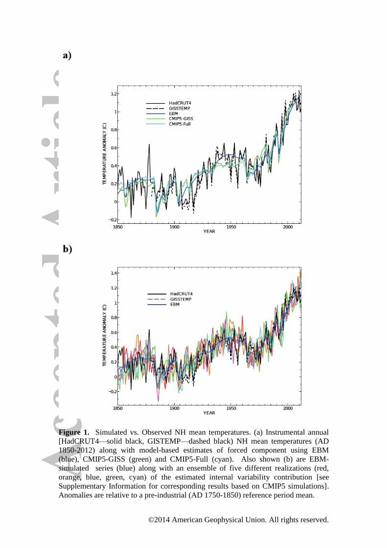
In Figure 1, we compare the model (EBM, CMIP5-GISS, and CMIP5-Full) estimates

of the purely forced component of Northern Hemisphere temperature from AD 1850-

present. We also show an ensemble of five NH mean surrogates produced using the

EBM simulation and five different noise (i.e. internal variability) realizations. The

HadCRUT4 [Brohan et al, 2006] and GISTEMP [Hansen et al, 2006] instrumental


NH annual mean (land+ocean) surface temperature series through AD 2012 are

shown for comparison.

It is apparent that the most recent decade is well within the ensemble spread. As we

have assumed a mid-range IPCC value of equilibrium climate sensitivity in the EBM

experiments, this latter observation argues against the notion that the slower rate of

warming over the past decade requires [e.g. as argued in The Economist, 2013] any

lowering of canonical ECS estimates. It is, instead, entirely consistent with the

expected level of multidecadal noise. Similar results are obtained (a) in other noise

ensembles, (b) varying the equilibrium climate sensitivity (ECS) over a wide range,

(c) using alternative aerosol ERF estimates, (d) varying aerosol scaling, (e) using

various alternative estimates of natural radiative forcing and (f) using CMIP5 model

estimates (both CMIP5-GISS and CMIP5-Full) in place of the EBM estimates

(Supplementary Information).

3.2. Hemispheric AMO Influence

In Figure 2 we show the estimated true historical realization of internal variability in

NH mean temperature, based on the Differenced-AMO approach (differencing the

observations and the model-estimated forced temperature series) using the EBM (Fig

2a), CMIP5-GISS (Fig 2b) and CMIP5-Full (Fig 2c) estimates of forced temperature

change. Also shown are the multidecadally-smoothed versions of the series, which

serve as estimates of the true NH mean projection of the AMO. We compare these

series with the residual series obtained by a linear detrending of the NH mean

temperature data followed by multidecadal smoothing, i.e. the NH mean projection of


the “AMO” series as estimated instead by the Detrended-AMO approach. The AMO

oscillation in the coupled model simulations of Knight et al [2005] was found to have

a NH mean amplitude A = 0.09 oC (standard error 0.02

oC). For a simple (i.e.

sinusoidal) oscillation, the root-mean-square deviation is related to the amplitude by σ

=A/√2. The Knight et al [2005] result thus gives a two standard error range σ = 0.064

+/- 0.028 oC. The AMO series estimated by the Differenced-AMO approach has a

root-mean-square deviation, σ =0.054 oC (EBM), σ =0.043

oC (CMIP5 GISS E2-R),

and σ =0.056 oC (CMIP5-Full), all within the uncertainty interval of the Knight et al

estimate. By contrast, the Detrended-AMO method yields a putative AMO signal with

σ =0.13 oC, twice as large as the Knight et al estimate, and well outside its two

standard error bounds.

An additional problem with the Detrended-AMO approach (as much an issue as the

amplitude overestimation) is the severe bias observed in the inferred phase of the

AMO. The Detrended-AMO series using either the EBM, CMIP5-GISS or CMIP5-

Full model estimate of the forced component, shows a substantial (~ -0.2 oC) negative

peak in the mid 1970s and a positive peak cresting at present. As noted in previous

work [Mann and Emanuel, 2006; Santer et al, 2006; Booth et al, 2012; Evan, 2012;

Dunstone et al, 2013] the former feature is almost certainly associated with the strong

anthropogenic sulphate aerosol cooling in the Northern Hemisphere from the 1950s-

1970s. Applying the Detrended-AMO approach directly to the model-estimated

forced component alone, we observe these same main features, including the 1950s-

1970s decrease (Figure 2). We conclude that those features arise from forced changes

in temperature rather than internal multidecadal variability.


The Differenced-AMO approach indeed suggests a very different AMO history,

regardless of whether the EBM, CMIP-GISS or CMIP-Full series is used to estimate

the forced component. Most importantly, a positive peak is now observed during the

1990s, with a subsequent decline through present (Figure 2). That decline is

associated with the much-discussed [The Economist, 2013; Allen et al, 2012; Stocker

et al, 2013] deficit of observed vs. model-predicted warming over the past decade. It

is thus reasonable to infer that the real AMO has played at least a modest role in that

deficit. To the extent that the AMO is an oscillatory mode, it is furthermore

reasonable to assume that this cooling effect is fleeting, and that the AMO is likely to

instead add to anthropogenic warming in the decades ahead.

Some recent studies indicate that initializing the state of the AMOC improves coupled

model hindcasts of North Atlantic warming since the mid 1990s [Yeager et al, 2012;

Msadek et al. 2013], which might appear to conflict with our finding of an AMO

cooling signal during this time frame. The improvement in skill, however, may simply

be a consequence of data assimilation, which serves to correct imperfect or missing

model physics by “nudging” the model toward the true climate state. Given “red

noise” climate persistence, such nudging guarantees that an initialized model will

exhibit more near-term skill than an uninitialized model, but it doesn’t tell us whether

the initial state assimilated into the model was primarily a result of internal variability,

forced variability, or some combination thereof.

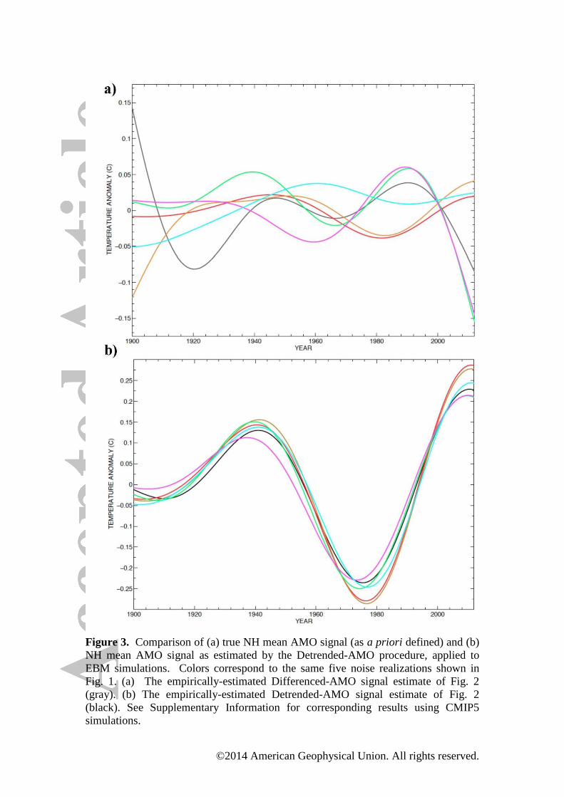
The biasing effect of the Detrended-AMO approach becomes even clearer when we

analyze the five synthetic alternative NH mean temperature realizations, and compare

(Fig. 3) the true AMO signal (which is known precisely in these cases since the


internal variability was specified a priori) and the Detrended-AMO signal. The true

AMO signals are—as they represent independent realizations of multidecadal noise—

uncorrelated among the five realizations (Fig. 3a). They are seen to have random

relative phase (i.e. random timings of negative and positive peaks), with typical peak

amplitude A ~0.1 oC. The random surrogates are qualitatively similar in their

attributes to the Differenced-AMO estimate of the real-world AMO series. By

contrast, the Detrended-AMO signals (Fig. 3b) show amplitudes A ~0.25 oC that are

inflated by more than a factor of two. Further, they are largely all in phase with the

Detrended-AMO signal diagnosed from observations (Fig. 2), an artifact of the

common forced signal masquerading as coherent low-frequency noise. The small

spread in phase among the different surrogates arises from the contribution of the true

random “AMO” variability shown in Fig 3a.

The above findings are robust (see Supplementary Information) with respect to

whether the EBM or two different CMIP5 (GISS and Full) forced NH mean

temperature estimates are used, and in the case of the EBM, the precise equilibrium

climate sensitivity, particular anthropogenic aerosol forcing series used, and

assumptions regarding the amplitude of indirect aerosol forcing.

3.3. “Stadium Waves”

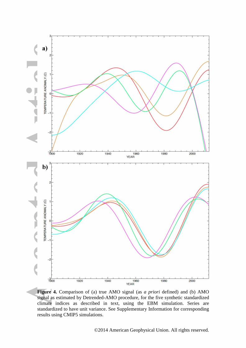
Finally, we examine the simulation of five AMO-related “indices”. Each index, as

noted earlier, has been degraded with an independent realization of additive white

noise to have a correlation of r=0.5 with the modeled NH mean temperature series,

and then smoothed to highlight multidecadal (greater than 50 year) timescale


variability. The multidecadal noise component is once again random and uncorrelated

across series by construction (Fig. 4a), so any “oscillation” that is coherent across the

five series must come instead from the common forced component. Indeed, the

Detrended-AMO approach (Fig. 4b) yields an apparent multidecadal “AMO”

oscillation that is coherent across the indices, an artifact of the residual forced signal

masquerading as an apparent low-frequency oscillation. The apparent “AMO” signal

is most coherent across indices during the most recent half century, when the forcing

is largest.

Another important feature apparent in this comparison is that the low-frequency noise

leads to substantial perturbations in the overall “phase” of the apparent “AMO” signal

(Fig. 4b) giving the appearance of a propagating wave or “stadium wave” in the

parlance of Wyatt et al [2012]. In previous work applying the Detrended-AMO

approach to estimate the “AMO” signal in a wide variety of climate indices [Wyatt et

al, 2012; Wyatt and Curry, 2013], such a feature was interpreted as an indication of an

AMO oscillation impacting a wide range of climate phenomena as it propagates

through the climate system. Our analysis suggests that this feature is instead an

artifact of the residual forced signal that remains after linear detrending (the

Detrended-AMO procedure), combined with random perturbations in the apparent

phase of the “oscillation” for any particular climate index, due to the low-frequency

effects of the additive noise.

Although the precise results depend (see Supplementary Information) on the

particular estimate (EBM, CMIP5-GISS or CMIP5-Full) used for the forced signal,

and in the case of the EBM, the assumed equilibrium climate sensitivity, as well as


the forcing series used and the amplitude of indirect effects assumed, the basic

conclusions above are once again robust with respect to all such details.

4. Conclusions

By comparing model-based estimates of forced temperature changes (using both an

EBM and ensemble means of the CMIP5 model simulations) with observed NH mean

temperatures over the historical era, we are able to empirically diagnose the internal

variability component of NH mean temperature. A simple statistical model applied to

that component is then used to generate an ensemble of noise realizations and an

ensemble of alternative NH mean temperature series. Actual NH mean

temperatures—including the temperature trend over the past decade—are shown to be

consistent with that ensemble. We conclude that there is no inconsistency between

recent observed and modeled temperature trends. As a corollary, recent temperature

observations are entirely consistent with prevailing mid-range estimates of climate

sensitivity.

We use the same ensemble to evaluate the faithfulness of the “Detrended Residual”

approach to estimating internal (AMO-related) variability, wherein temperature data

are linearly detrended, the residual is interpreted as internal variability, and the

multidecadal component of the residual is interpreted as representing a low-frequency

“AMO” oscillation. In cases where the signal is known a priori, we show that this

procedure yields a biased estimate of the true AMO signal in the data. The procedure

attributes too large an amplitude to the AMO signal and a biased estimate of its phase.

Wherein application of the flawed Detrended-AMO approach attributes some of the


recent NH mean temperature rise to an AMO signal, the true AMO signal instead

appears likely to have contributed to a relative cooling over the past decade,

explaining some of the observed slowing of warming during that timeframe. We find

that claims of a “stadium wave” AMO signal propagating through the global climate

are likely an artifact of the Detrended-AMO procedure as well.

Acknowledgements:

All raw data, ©Matlab code, and results from our analysis are available at the

supplementary website:

http://www.meteo.psu.edu/~mann/supplements/GRL_AMO14. We thank Drew

Shindell, Ron Miller, Larisa Nazarenko and Gavin Schmidt of NASA/GISS for input

regarding aerosol forcing estimates and provision of the GISS NINT aerosol forcing

series. BAS acknowledges the U.S. National Science Foundation AGS-PRF (AGS-

1137750). We also thank the two anonymous reviewers of the manuscript for their

helpful comments.

References

Allen, M. R., J. F. B. Mitchell, and P. A. Stott (2013), Test of A Decadal Climate

Forecast, Nat. Geosci., 6, 243–244.

Booth, B. B. B., N. J. Dunstone, P. R. Halloran, T. Andrews, and N. Bellouin (2012),

Aerosols implicated as a prime driver of twentieth-century North Atlantic climate variability,

Nature, 484, 228–232.

http://www.meteo.psu.edu/~mann/supplements/GRL_AMO14


Boucher et al. (2013) Clouds and Aerosols. In Climate change 2013: the physical

science basis. Working Group I contribution to the Fifth Assessment Report of the

Intergovernmental Panel on Climate Change (eds. Stocker et al.).

Brohan, P., J. J. Kennedy, I. Haris, S. F. B. Tett, and P. D. Jones (2006), Uncertainty

estimates in regional and global observed temperature changes: a new dataset from

1850, J. Geophys. Res., 111, D12106, doi:10.1029/2005JD006548.

Carslaw et al. (2013), Large contribution of natural aerosols to uncertainty in indirect

forcing, Nature, 503, 67-71.

Delworth, T., S. Manabe, and R. J. Stouffer (1993), Interdecadal variations of the

thermohaline circulation in a coupled ocean-atmosphere model, J. Clim., 6, 1993–

2011.

Delworth, T. L., S. Manabe, and R. J. Stouffer (1997), Multidecadal climate

variability in the Greenland Sea and surrounding regions: A coupled model

simulation, Geophys. Res. Lett., 24, 257–260.

Delworth, T. L., and M. E. Mann (2000), Observed and Simulated Multidecadal

Variability in the Northern Hemisphere, Clim. Dynam., 16, 661–676.

Delworth, T. L., R. Zhang, and M. E. Mann (2007), Decadal to Centennial Variability

of the Atlantic from Observations and Models, in Past and Future Changes of the

Oceans Meridional Overturning Circulation: Mechanisms and Impacts, Geophys.


Monogr. Ser., vol. 173, edited by A. Schmittner, J. C. H. Chiang, and S. R. Hemming,

pp.131–148, AGU, Washington, D. C.

Dunstone N. J, D. M. Smith, B. B. B. Booth, L. Hermanson, and R. Eade (2013),

Anthropogenic aerosol forcing of Atlantic tropical storms, Nat. Geosci., 6, 534–539,

doi:10.1038/NGEO1854.

Enfield, D. B., A. M. Mestas-Nuñez, and P. J. Trimble (2001), The Atlantic

multidecadal oscillation and its relation to rainfall and river flows in the continental

US, Geophys. Res. Lett., 28, 2077–2080.

Evan, A. (2012), Aerosols and Atlantic aberrations, Nature, 484, 170–171.

doi:10.1038/nature11037, 2012.

Flato et al. (2013) Evaluation of Climate Models. In Climate change 2013: the

physical science basis. Working Group I contribution to the Fifth Assessment Report

of the Intergovernmental Panel on Climate Change (eds. Stocker et al.).

Folland, C. K., D. E. Parker, and F. E. Kates (1984), Worldwide marine temperature

fluctuations 1856-1981, Nature, 310, 670–673.

Folland, C. K., D. E. Parker, and T. N. Palmer (1986), Sahel rainfall and worldwide

sea temperatures 1901–85, Nature, 320, 602–607.


Goldenberg, S. B., C. W. Landsea, A. M. Mestas-Nuñez, and W. M. Gray (2001), The

recent increase in Atlantic hurricane activity: Causes and implications, Science, 293,

474–479.

Hansen, J., Mki. Sato, R. Ruedy, K. Lo, D.W. Lea, and M. Medina-Elizade, 2006:

Global temperature change. Proc. Natl. Acad. Sci., 103, 14288-14293,

doi:10.1073/pnas.0606291103.

Hurrell, J. W. (1996), Influence of Variations in Extratropical Wintertime

Teleconnections on Northern Hemisphere Temperature, Geophys. Res. Lett., 23, 665–

668.

Kerr, R. A. (2000), A North Atlantic climate pacemaker for the centuries, Science,

288, 1984–1985.

Knight, J. R., R. J. Allan, C. K. Folland, M. Vellinga, and M. E. Mann (2005), A

Signature of Persistent Natural Thermohaline Circulation Cycles in Observed

Climate, Geophys. Res. Lett., 32, L20708, doi: 10.1029/2005GL02423.

Koch, D. et al. (2011), Coupled aerosol-chemistry-climate twentieth century transient

model investigation: Trends in short-lived species and climate responses. J. Climate,

24, 2693–2714, doi:10.1175/2011JCLI3582.

Kushnir, Y. (1994), Interdecadal variations in North Atlantic sea surface temperature

and associated atmospheric conditions, J. Clim., 7, 141–157.


Mann, M. E. (2008), Smoothing of Climate Time Series Revisited, Geophys. Res.

Lett., 35, L16708, doi:10.1029/2008GL034716.

Mann, M. E. (2011), On Long Range Dependence in Global Surface Temperature

Series, Climatic Change, 107, 267–276.

Mann, M. E. (2012), The Hockey Stick and the Climate Wars, Columbia University

Press, New York, N. Y., pp. 384.

Mann, M. E., and J. Park (1994), Global-scale modes of surface temperature

variability on interannual to century timescales, J. Geophys. Res., 99, 819–833.

Mann, M. E., J. Park, and R. S. Bradley (1995), Global interdecadal and century-scale

climate oscillations during the past 5 centuries, Nature, 378, 266–270.

Mann, M. E., and J. Park (1996), Joint Spatio-Temporal Modes of Surface

Temperature and Sea Level Pressure Variability in the Northern Hemisphere During

the Last Century, J. Clim., 9, 2137–2162.

Mann, M. E., and K. A. Emanuel (2006), Atlantic Hurricane Trends linked to Climate

Change, Eos, 87(24), 233–241.


Mann, M. E., J. D. Fuentes, and S. Rutherford (2012), Underestimation of Volcanic

Cooling in Tree-Ring Based Reconstructions of Hemispheric Temperatures, Nat.

Geosci., 5, 202–205.

Msadek, R., W. E. Johns, S. G. Yeager, G. Danabasoglu, T. L. Delworth, and A.

Rosati, (2013),,The Atlantic meridional heat transport at 26.5ºN and its relationship

with the MOC in the RAPID array and the GFDL and NCAR coupled models J.

Climate, 26, 4335–4356.

North, G. R., R. F. Cahalan, and J. A. Coakley (1981), Energy balance climate

models, Rev. Geophys., 19, 91–121.

Santer, B. D., T. M. L. Wigley, P. J. Gleckler, C. Bonfils, M. F. Wehner, K.

AchutaRao, T. P. Barnett, J. S. Boyle, W. Brüggemann, M. Fiorino, N. Gillett, J. E.

Hansen, P. D. Jones, S. A. Klein, G. A. Meehl, S. C. B. Raper, R. W. Reynolds, K. E.

Taylor, and W. M. Washington (2006), Forced and unforced ocean temperature

changes in Atlantic and Pacific tropical cyclogenesis regions, Proc. Natl. Acad. Sci.

USA, 103, 905–910.

Schlesinger, M. E., and N. Ramankutty (1994), An oscillation in the global climate

system of period 65– 70 years, Nature, 367, 723–726.

Stevens, B. (2013), Aerosols: Uncertain then, irrelevant now, Nature, 503, 47–48.


Stocker et al. (2013) Climate Change 2013: The Physical Science Basis - Summary

for Policymakers. In Climate change 2013: the physical science basis. Working Group

I contribution to the Fifth Assessment Report of the Intergovernmental Panel on

Climate Change (eds. Stocker et al.).

Ting, M., Y. Kushnir, R. Seager, and C. Li (2009), Forced and internal twentieth-

century SST trends in the North Atlantic, J. Clim., 22, 1469–1481.

Trenberth, K. E., and D. J. Shea (2006), Atlantic hurricanes and natural variability in

2005, Geophys. Res. Lett., 33, L12704, doi:10.1029/2006GL026894.

The Economist (editorial), “A Sensitive Matter”, March 30, 2013.

http://www.economist.com/news/science-and-technology/21574461-climate-may-be-

heating-up-less-response-greenhouse-gas-emissions

Wyatt, M. G., S. Kravtsov, and A. A. Tsonis (2012), Atlantic multidecadal Oscillation

and Northern Hemisphere’s climate variability, Clim. Dynam., 38(5–6), 929–949.

doi:10.1007/s00382-011-1071-8.

Wyatt, M. G., and J. A. Curry (2013), Role for Eurasian Arctic shelf sea ice in a

secularly varying hemispheric climate signal during the 20th century, Clim. Dynam.,

doi: 10.1007/s00382-013-1950-2.


Yeager, S., A. Karspeck, G. Danabasoglu, J. Tribbia, and H. Teng (2012), A Decadal

Prediction Case Study: Late Twentieth-Century North Atlantic Ocean Heat Content.

J. Climate, 25, 5173–5189.


Figure 1. Simulated vs. Observed NH mean temperatures. (a) Instrumental annual

[HadCRUT4—solid black, GISTEMP—dashed black) NH mean temperatures (AD

1850-2012) along with model-based estimates of forced component using EBM

(blue), CMIP5-GISS (green) and CMIP5-Full (cyan). Also shown (b) are EBM-

simulated series (blue) along with an ensemble of five different realizations (red,

orange, blue, green, cyan) of the estimated internal variability contribution [see

Supplementary Information for corresponding results based on CMIP5 simulations].

Anomalies are relative to a pre-industrial (AD 1750-1850) reference period mean.


Figure 2. Time series of estimated unforced NH mean variability (annual series) and

associated multidecadal “AMO” components (smooth curves) based on Differenced-

AMO (gray) vs. Detrended-AMO (black) approaches applied to the observational NH

mean record, using (a) EBM simulation, (b) CMIP5-GISS and (c) CMIP5-Full.

Shown for comparison (blue) is the Detrended-AMO approach applied to the model-

simulated forced series alone. For CMIP5 cases (i.e. b. and c.) the model series end in

2005 but have been extended to 2012 by persistence of the 30 year trend. Similar

results are obtained based on persistence of the 2005 value [see Supplementary

Information].


Figure 3. Comparison of (a) true NH mean AMO signal (as a priori defined) and (b)

NH mean AMO signal as estimated by the Detrended-AMO procedure, applied to

EBM simulations. Colors correspond to the same five noise realizations shown in

Fig. 1. (a) The empirically-estimated Differenced-AMO signal estimate of Fig. 2

(gray). (b) The empirically-estimated Detrended-AMO signal estimate of Fig. 2

(black). See Supplementary Information for corresponding results using CMIP5

simulations.


Figure 4. Comparison of (a) true AMO signal (as a priori defined) and (b) AMO

signal as estimated by Detrended-AMO procedure, for the five synthetic standardized

climate indices as described in text, using the EBM simulation. Series are

standardized to have unit variance. See Supplementary Information for corresponding

results using CMIP5 simulations.

Documents

On Forced Temperature Changes, Internal … Forced Temperature Changes, Internal Variability and the AMO Michael E. Mann Byron A. Steinman Sonya K. Miller Department of Meteorology