Embed Size (px)
Citation preview
111
On Fundamental Principles for Thermal-Aware Design onPeriodic Real-Time Multi-Core Systems
SHI SHA,Wilkes University, USA
AJINKYA S. BANKAR, Florida International University, USAXIAOKUN YANG, University of Houston Clear Lake, USA
WUJIE WEN, Lehigh University, USA
GANG QUAN, Florida International University, USA
With the exponential rise of the transistor count in one chip, the thermal problem has become a pressing
issue in computing system design. While there have been extensive methods and techniques published for
design optimization with thermal awareness, there is a need for more rigorous and formal thermal analysis
in designing real-time systems and applications that demand a strong exception guarantee. In this paper,
we analytically prove a series of fundamental properties and principles concerning RC thermal model, peak
temperature identification and peak temperature reduction for periodic real-time systems, which are general
enough to be applied on 2D and 3D multi-core platforms. These findings enhance the worst-case temperature
predictability in runtime scenarios, help to develop more effective thermal management policy, which is key
to thermal-constrained periodic real-time system design.
CCS Concepts: • Computer systems organization → Embedded systems; Multicore architectures; Real-time operating systems; Real-time system architecture; • Hardware → Temperature simulation and esti-mation; Temperature control; Temperature optimization.
Additional Key Words and Phrases: multi-core architecture; thermal-aware design; temperature bound; peak
temperature minimization; dynamic thermal management (DTM); dynamic voltage frequency scaling (DVFS);
worst- case execution time (WCET).
ACM Reference Format:Shi Sha, Ajinkya S. Bankar, Xiaokun Yang, Wujie Wen, and Gang Quan. 2018. On Fundamental Principles for
Thermal-Aware Design on Periodic Real-Time Multi-Core Systems. ACM Trans. Des. Autom. Electron. Syst. 37,4, Article 111 (August 2018), 31 pages. https://doi.org/10.1145/1122445.1122456
1 INTRODUCTIONThe advancement of IC technology has changed human life and society profoundly, largely due to
the tremendous progress of computing systems ranging from large-scale data centers to daily used
mobile devices. However, the semiconductor industry development is now reaching a saturation
point of Moore’s Law due to high power consumption and heat dissipation, among other factors.
Authors’ addresses: Shi Sha, [email protected], Wilkes University, 84 W. South Street, Wilkes-Barre, Pennsylvania, 18766,
USA; Ajinkya S. Bankar, [email protected], Florida International University, 10555 West Flagler Street, EC3900, Miami,
Florida, 33174, USA; Xiaokun Yang, [email protected], University of Houston Clear Lake, 2700 Bay Area Blvd, Houston,
Texas, 77058, USA; Wujie Wen, [email protected], Lehigh University, 19 Memorial Drive W., Bethlehem, Pennsylvania,
18015, USA; Gang Quan, [email protected], Florida International University, 10555 West Flagler Street, EC3900, Miami,
Florida, 33174, USA.
Permission to make digital or hard copies of all or part of this work for personal or classroom use is granted without fee
provided that copies are not made or distributed for profit or commercial advantage and that copies bear this notice and
the full citation on the first page. Copyrights for components of this work owned by others than ACM must be honored.
Abstracting with credit is permitted. To copy otherwise, or republish, to post on servers or to redistribute to lists, requires
prior specific permission and/or a fee. Request permissions from [email protected].
© 2018 Association for Computing Machinery.
1084-4309/2018/8-ART111 $15.00
https://doi.org/10.1145/1122445.1122456
ACM Trans. Des. Autom. Electron. Syst., Vol. 37, No. 4, Article 111. Publication date: August 2018.
111:2 Sha and Bankar, et al.
The soaring power and accompanied thermal crisis negatively impacts the system computational
performance, reliability, shortens devices lifespan or even damages the processor permanently.
Temperature has become one of the primary concerns in modern microprocessor design and the
thermal environment is becoming even worse in many-core and 3D architectures.
While it is a common practice to limit the power consumption – using so-called thermal designpower (TDP) – to ensure that thermal issues are under control, the challenges of temperature
management on 2D or 3D multi-core platform come from not only the high power dissipation, but
also the uneven heat dissipation temporally and spatially. For example, on an Intel Xeon E5-2699
v3 CPU [5], the intra-die temperature difference can be up to 10C and 24
C under balanced and
unbalanced workload scenarios, respectively. In addition, thermal nodes with longer heat removal
paths in 3D architecture exacerbate the thermal gradient. Therefore, conventional power budgeting
on multi-core platforms become insufficient in thermal guarantee [39].
To reduce the chip temperature, mechanical cooling solutions, e.g. thermal-aware floor-planning,
heat removal fan and micro-channel liquid cooling, fall short to many computing systems, es-
pecially the mobile ones. Alternatively, dynamic thermal management (DTM) is widely accepted
as an effective solution both in design and runtime to smooth the thermal gradient by dynamicvoltage frequency scaling (DVFS), or to shut down the unused cores by dynamic power manage-ment (DPM) [48].
Many DTM strategies are proposed, such as thermal-balancing [34], “hot-and-cold” job swap-
ping [41], allocating hot tasks to cores closer to the heat sink [29], etc. These heuristic approaches
developed cannot guarantee the temperature constraint in computing system design. There are
also other approaches that resort to traditional control and optimization methods, such as feedback
control [4, 19], machine learning [12, 15], mathematical programming [23, 54]. While some of these
approaches, e.g. the runtime learning approach in [15], can guarantee the temperature constraints,
it could be extremely challenging when employing the above approach to ensure both the timing
and peak temperature constraints for real-time systems with complicated scheduling policies.
To facilitate more rigorous analytical thermal analyses, which we believe is indispensable for
system level thermal-aware real-time system design, we intend to develop general and provable
principles and fundamentals on characteristics of heat dissipation for ease of formal verification
and analysis. The contribution of this paper includes:
• First, we introduce a series of provable lemmas and theorems, which unveil some interesting
characteristics of the complex RC-thermal model and facilitate more formal analytical thermal-
aware analyses and design on multi-core platforms;
• Second, peak temperature plays a critical role in the thermal-aware periodic real-time system
design, but identifying the peak temperature on multi-core platforms is non-trivial. In this
paper, we propose to employ the so-called “step-up execution trace” to quickly and effectively
bound the peak temperature for periodic real-time systems, i.e. the commonly used real-time
system model, and formally prove its validity. Our proposed method can be broadly adopted
in real-time systems design when developing both online and offline thermal management
policies;
• Third, it is known that on a single-core platform, splitting the taskswith different power/thermal
characteristics into multiple sections and executing them interchangeably, namely frequencyoscillating, can reduce the peak temperature [25]. However, we find that applying such a
mechanism on one core or on a part of the chip cannot always reduce the peak temperature
on multi-core platforms. Instead, we develop the multi-core “m-Oscillating” method and
formally prove that it can reduce the overall peak temperature. Moreover, we also prove
ACM Trans. Des. Autom. Electron. Syst., Vol. 37, No. 4, Article 111. Publication date: August 2018.

On Fundamental Principles for Thermal-Aware Design on Periodic Real-Time Multi-Core Systems111:3
that the “m-Oscillating” can enhance the system’s real-time service throughput under peak
temperature constraints in the real-time domain.
These conclusions can be applied to both online and offline design stages and address the urgent
demands of runtime performance/thermal guarantees in the real-time system design. They are also
general enough to be applied on 2D, 3D multi-core platforms and other linear-time-invariant (LTI)
systems that may be of interest from a temperature-aware standpoint.
2 RELATEDWORKSThere have been extensive research efforts for thermal related optimizations onmulti-core platforms,
including throughput maximization (e.g. [13, 35, 45, 54]), power/energy reduction (e.g. [37, 42, 56]),
peak temperature reduction (e.g. [8, 14, 57]) and reliability enhancement (e.g. [52]), etc. Essentially,
these works aim at optimizing the resource usage in design of high performance, low power/energy
and highly reliable computing systems with chip temperature either as an optimization goal or a
design constraint. Based on different methodologies, the existing work can be largely classified
into the following three categories.
First, many heuristic methods rely on extensive testing and hand-tuning. For example, several
solutions have been proposed for the peak temperature minimization problem, including interleav-
ing the hot/cool tasks in 3D platforms temporally and spatially [29], assigning slacks to split hot
tasks [57] and associating active cooling with task assignment [5]. However, in these approaches,
to determine the accurate and strongly justifiable metrics to classify hot/cool tasks/cores can be
difficult. In addition, without capturing solid analytical correlations, it can be challenging to make
other design tradeoffs in the meantime, such as task migration overhead vs. scheduling intervallength. Although these heuristic/intuition methods may work in some application scenarios, it
becomes extremely difficult, if not impossible at all, to guarantee the system performance and
design constraints such as timing and peak temperature.
Second, some other approaches resort to traditional control techniques [4, 19] or optimization
methods, such as machine learning [15], mathematical programming or meta-heuristic searching
methods [55], to deal with thermal issues. For example, using feedback control techniques on
multi-core platforms, Bartolini et al. [4] proposed a feedback control framework to enforce thermal
control, energy minimization and thermal model self-calibration. Hanumaiah et al. [19] developed a
closed-loop controller to predict the desired voltage/frequency settings to achieve maximum energy
efficiency without violating the thermal limitations. Xie et al. [55] developed a look-up table based
DTM method on a thermal coupled processor/battery model to achieve the maximal throughput.
These approaches help to uncover the rationales in temperature management. However, it is still
difficult to strongly guarantee the temperature constraints due to the inaccurate sensor-based
temperature reading and control.
Themathematical programmingmethods are also employed to optimize resource allocation under
temperature and other design constraints. For example, the throughput maximization problem on
a temperature-constrained multi-core platform has been studied by the linear programming (LP)
approach in [54], and by a convex optimization method in [35]. However, [35] ignores the lateral
heat transfer among different cores. Other approaches, such as mixed-integer linear programming
(MILP), have been used to minimize the peak temperature in [8], or reduce the peak temperature
and energy contemporarily for video streaming in [49]. A genetic programming approach has
been proposed to minimize the energy consumption for periodic tasks under a peak temperature
constraint in [42]. A meta-heuristic approach has been proposed to boost system performance in a
small interval by supplying additional power to the system without exceeding the temperature
and power supply limit in [13]. These mathematical programming-based approaches can provide
ACM Trans. Des. Autom. Electron. Syst., Vol. 37, No. 4, Article 111. Publication date: August 2018.
111:4 Sha and Bankar, et al.
a solution, but it cannot qualitatively express the impacts between different variables and the
optimization goals. In addition, the computational costs of many mathematical programming-based
solutions, e.g. [8, 49, 54], increase too fast and can be prohibitive as the system scale becomes larger
in future many-core processors.
The third type of approaches (e.g. [2, 14, 39, 45, 55]) intend to ensure a strong guarantee to
thermal constraints based on formal and analytical thermal analysis, to uncover underlying corre-
lations among different design parameters quantitatively and not qualitatively. This is particularly
useful in the design of real-time systems, where predictability is critical and complicated resource
management policies (such as priority, preemption, resource sharing, etc) cannot be easily formu-
lated in mathematical programming. For example, a thermal-aware global scheduling algorithm for
sporadic task sets has been proposed in [14]; the energy optimization under a given temperature
constraint has been solved by a convex method in [22] and by a variable-sized bin packing approach
in [44]; the throughput maximization problem has been studied in [21, 23]; the reliability has
been enhanced in [20]. However, since [14, 20–23] incorrectly assume the peak temperature only
occurred at a scheduling point and [20, 21, 23] ignore the lateral heat transfer among different
cores, the inaccurate peak temperature prediction may trigger the DTM or even shut down the
processors, which may lead to a real-time violation. To achieve higher computational capacity, the
thermal safe power (TSP) has been proposed in [39], which achieves a higher power budget than
the traditional thermal design power (TDP). Sha et al. [45] present a frequency oscillating method
to maximize the throughput with a guaranteed peak temperature on a multi-core platform. Assisted
with rigorous mathematical analysis, these approaches help to uncover fundamental principles
for more efficient and effective thermal-aware design, which would be otherwise unavailable.
Moreover, the formal analytical analyses do not suffer from prohibitive computational cost in many
mathematical programming approaches.
In this paper, based on the traditional RC-thermal model for multi-core platforms, we present a
series of analyses on thermal models, peak temperature identification and reduction, which we
believe can greatly enhance the formal analytical research on thermal-constrained design problem
on multi-core platforms. The rest of this paper is organized as follows. Section III introduces
the multi-core system and thermal models. Section IV studies the general principle of the RC-
thermal model. Peak temperature bound and minimization is discussed in Section V and Section VI,
respectively. Section VII shows the experiment results and is followed by a conclusion in Section VIII.
3 PRELIMINARIESWe present the models for our multi-core systems. The bold characters represent the vectorsand matrices and non-bold characters are used for ordinary variables and coefficients. All the
matrices/vectors/values are in the real number domain. The notations in Table 1 are used in the
paper.
3.1 System ModelWe consider a multi-core platform. Each processing core is DVFS-independent. Each core has
different running modes and each running mode is characterized by a pair of parameters (𝑣, 𝑓 ),where 𝑣 is the supply voltage and 𝑓 is the working frequency (𝑣 ∝ 𝑓 ). For an idle core, we assume
𝑣 = 𝑓 = 0 and for an inactive node ( such as heat sink/spreader), we assume there is no power
consumption. In this paper, for ease of presentation, we use supply voltage 𝑣 to denote the processing
speed (amount of work performed within a unit time) when there is no confusion.
As different cores may execute in different runningmodes at different times, a multi-core platform
can be regarded as running on a sequence of scheduling intervals, in each of which each core runs
only in a unique mode. We call such an interval, e.g. [𝑡𝑞−1, 𝑡𝑞], as a state interval.
ACM Trans. Des. Autom. Electron. Syst., Vol. 37, No. 4, Article 111. Publication date: August 2018.
On Fundamental Principles for Thermal-Aware Design on Periodic Real-Time Multi-Core Systems111:5
Table 1. Summary of Notations
Symbol Meaning𝑁 Total number of thermal nodes;
S(𝑡) A periodic multi-core schedule;
I𝑞 The 𝑞𝑡ℎ state interval in S(𝑡) with time interval [𝑡𝑞−1, 𝑡𝑞];𝑙𝑞 The interval length of I𝑞 , i.e. 𝑙𝑞 = 𝑡𝑞 − 𝑡𝑞−1;v𝑞 The supply voltage of the 𝑞𝑡ℎ state interval;
T0 The starting temperatures;
T𝑠𝑠 (𝑡) The stable status temperatures at time 𝑡 ;
T𝑝𝑒𝑎𝑘 (S(𝑡)) The peak temperatures of running S(𝑡);T∞𝑞 The constant temperature when running processor using supply voltage v𝑞
long enough to enter the stable state;
1𝑁×1 An (𝑁 × 1) matrix with all elements being 1;
0𝑁×1 An (𝑁 × 1) matrix with all elements being 0;
𝑚𝑎𝑥 (X) Find the maximum scalar value from matrix/vector X;
Given two matrices X and Y with the same dimensions (e.g. 𝑁1 × 𝑁2 ), operators > , < , ≥and ≤ are defined as element-wise scalar comparisons. For example, X ≤ Y means that
𝑋𝑖, 𝑗 ≤ 𝑌𝑖, 𝑗 , ∀𝑖 ∈ [1, 𝑁1] and ∀𝑗 ∈ [1, 𝑁2].
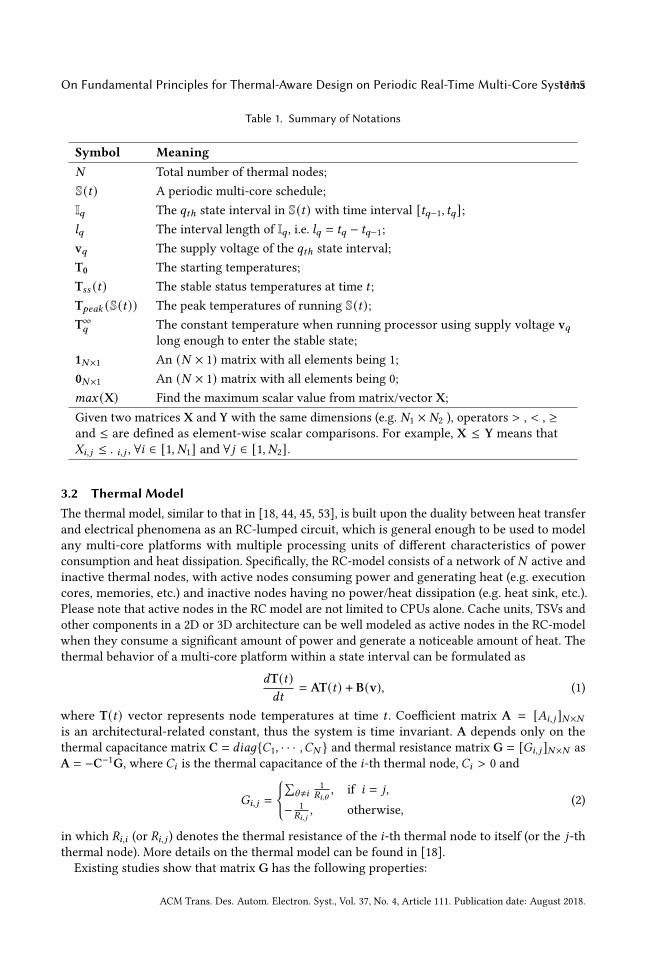
3.2 Thermal ModelThe thermal model, similar to that in [18, 44, 45, 53], is built upon the duality between heat transfer
and electrical phenomena as an RC-lumped circuit, which is general enough to be used to model
any multi-core platforms with multiple processing units of different characteristics of power
consumption and heat dissipation. Specifically, the RC-model consists of a network of 𝑁 active and
inactive thermal nodes, with active nodes consuming power and generating heat (e.g. execution
cores, memories, etc.) and inactive nodes having no power/heat dissipation (e.g. heat sink, etc.).
Please note that active nodes in the RC model are not limited to CPUs alone. Cache units, TSVs and
other components in a 2D or 3D architecture can be well modeled as active nodes in the RC-model
when they consume a significant amount of power and generate a noticeable amount of heat. The
thermal behavior of a multi-core platform within a state interval can be formulated as
𝑑T(𝑡)𝑑𝑡
= AT(𝑡) + B(v), (1)
where T(𝑡) vector represents node temperatures at time 𝑡 . Coefficient matrix A = [𝐴𝑖, 𝑗 ]𝑁×𝑁is an architectural-related constant, thus the system is time invariant. A depends only on the
thermal capacitance matrix C = 𝑑𝑖𝑎𝑔𝐶1, · · · ,𝐶𝑁 and thermal resistance matrix G = [𝐺𝑖, 𝑗 ]𝑁×𝑁 as
A = −C−1G, where 𝐶𝑖 is the thermal capacitance of the 𝑖-th thermal node, 𝐶𝑖 > 0 and
𝐺𝑖, 𝑗 =
∑\≠𝑖
1
𝑅𝑖,\, if 𝑖 = 𝑗,
− 1
𝑅𝑖,𝑗, otherwise,
(2)
in which 𝑅𝑖,𝑖 (or 𝑅𝑖, 𝑗 ) denotes the thermal resistance of the 𝑖-th thermal node to itself (or the 𝑗-th
thermal node). More details on the thermal model can be found in [18].
Existing studies show that matrix G has the following properties:
ACM Trans. Des. Autom. Electron. Syst., Vol. 37, No. 4, Article 111. Publication date: August 2018.

111:6 Sha and Bankar, et al.
Property 1. Matrix G has the following properties:(1) G is a quasi-positive matrix with all of its entries being non-negative except for those on the
main diagonal [18];(2) G is strictly diagonally dominant, real symmetric and nonsingular (Lemma 1 in [53]);
Both C and G are 𝑁 × 𝑁 square matrices. Since C only contains non-zero elements on the
diagonal, it is invertible. Moreover, G is also invertible, because it is nonsingular. Then, sinceA · A−1 = −C−1G · (−C−1G)−1 = C−1GG−1C = I, A is invertible. A is neither symmetric nor
diagonal dominant.
Coefficient vector B = [𝐵𝑖 ]𝑁×1, a power-related vector, depends on not only the thermal ca-
pacitances of the multi-core platform but also the running mode of each active thermal node. It
is reasonable to assume that ∀v1 ≥ v2 leads to B(v1) ≥ B(v2). The power-related vector B does
not make any assumption on power parameters, so it is general enough to adopt different power
models. In this paper, we take leakage-temperature dependency [18, 44] on the active processing
units into accounts in Section 7.
When running a multi-core processor under a constant supply voltage v long enough (i.e.
𝑡 → ∞), it will eventually reach a constant temperature T∞ (v) = −A−1B(v) as 𝑑T(∞)/𝑑𝑡 = 0. Forschedules that consist of multiple state intervals, the state intervals may not be long enough for
the temperature to be constant. As shown in [18], the transient temperature at time 𝑡 within a state
interval (e.g. the 𝑞-th interval [𝑡𝑞−1, 𝑡𝑞]) can be formulated as
T(𝑡) = 𝑒A(𝑡−𝑡𝑞−1)T(𝑡𝑞−1) + (I − 𝑒A(𝑡−𝑡𝑞−1) )T∞𝑞 , (3)
where 𝑡𝑞−1 ≤ 𝑡 ≤ 𝑡𝑞 and T(𝑡𝑞−1) is the temperature vectors at the beginning of the 𝑞-th interval.
T∞𝑞 is the constant temperature when running processor using supply voltage v𝑞 long enough to
enter the stable state and I is an identity matrix.
When repeating a periodic schedule with multiple state intervals long enough, the temperature
eventually enters the thermal stable status, in which the temperature trace exhibits a repeat pattern.
Specifically, for a periodic schedule S(𝑡) with 𝑧 state intervals and period 𝑡𝑝 , let 𝑡𝑞−1 and 𝑡𝑞 be the
starting time and ending time of the 𝑞-th state interval, respectively. The transient temperature in
the stable status can be formulated as [18]
T𝑠𝑠 (𝑡𝑞) = T(𝑡𝑞) + K𝑞 (I − K)−1 (T(𝑡𝑝 ) − T(0)), (4)
in which T(𝑡𝑞) and T𝑠𝑠 (𝑡𝑞) are the temperatures at time 𝑡𝑞 in the first period and that in the thermalstable status, respectively. T(0) is the starting temperature for the first period and equals to T0.
The \ -th state interval size 𝑙\ = 𝑡\ − 𝑡\−1, K𝑞 = 𝑒A∑𝑞
\=1𝑙\and K = 𝑒A
∑𝑧\=1
𝑙\ = 𝑒A𝑡𝑝. A more detailed
explanation of the notations and equations can be found in [18].
4 THE PROPERTIES OF THE THERMAL MODELIn this section, we focus on some inherent properties related to the multi-core RC thermal model
itself. We believe that a better understanding of the thermal models helps to develop more effective
thermal management policies in computing systems design.
The thermal model in (1) is a linear time-invariant (LTI) system, which captures the thermal
dynamics by 𝑁 first-order differential equations involving 𝑁 state variables. The system matrix Aplays a vital role in determining temperature dynamics according to the transient power dissipation
in runtime. Note that A affects how current temperature influences the future temperature change
in 𝑑T(𝑡)/𝑑𝑡 [18] and A also affects the stable state temperature in T∞. Moreover, the properties
of A determine the system stability [6], and its transformations, such as −A−1, 𝑒A𝑙
or (I − 𝑒A𝑙 )−1,etc, are closely related to other properties of a system. To better understand the properties related
ACM Trans. Des. Autom. Electron. Syst., Vol. 37, No. 4, Article 111. Publication date: August 2018.

On Fundamental Principles for Thermal-Aware Design on Periodic Real-Time Multi-Core Systems111:7
to matrix A, we present several important lemmas and theorems as follows. In this paper, all the
detailed proofs can be found in the Appendix, if otherwise specified.
Lemma 4.1. Matrix A has all negative real eigenvalues.
Lemma 4.2. Matrix A is diagonalizable.
Lemma 4.3. Matrix A is constant and all the entries of −A−1 = [A𝑖, 𝑗 ]𝑁×𝑁 are positive real numbersand A𝑖, 𝑗 > 0.
In control theory, a system is asymptotically stable [7], if all the eigenvalues of the system matrix
are strictly negative real values. An asymptotically stable system is bounded-input, bounded-output
(BIBO) stable, which means that the output will be bounded for every input to the system that is
bounded. Therefore, from Lemma 4.1, there always exists a peak temperature for any schedule
executed on a given platform, with its power supply stay below the maximal threshold.
Since A is diagonalizable (Lemma 4.2) and all of its eigenvalues are negative (Lemma 4.1), we
can easily calculate its eigenvalues. Let −_𝑖 be the i-th eigenvalue of A and _𝑖 > 0, we have
A = WDW−1, where D = 𝑑𝑖𝑎𝑔−_1, · · · ,−_𝑁 and W = [ ®𝑤1, · · · , ®𝑤𝑁 ]. ®𝑤𝑖 is the independent
eigenvectors associated with −_𝑖 . The matrix exponential of 𝑒A𝑙can be diagonalized as
𝑒A𝑙 =
∞∑ℎ=0
𝑙ℎ (WDW−1)ℎℎ!
= W( ∞∑ℎ=0
𝑙ℎDℎ
ℎ!
)W−1 = W𝑒D𝑙W−1, (5)
where 𝑒D𝑙 = 𝑑𝑖𝑎𝑔𝑒−_1𝑙 , · · · , 𝑒−_𝑁 𝑙 and 𝑒−_𝑖𝑙 is the 𝑖-th eigenvalue of 𝑒A𝑙.
In addition, since none of the eigenvalue ofA equal to zero (Lemma 4.1), matrixA is invertible. The
negative inverted matrix −A−1plays an important role in determining the stable state temperature
T∞ (v), which, in turn, impacts the thermal dynamics in (3). This attribute of −A−1in Lemma 4.3
also enables the comparison of the stable state temperatures of different constant running modes.
In particular, since power consumption is proportional to the supply voltages of different running
modes, i.e. ∀v1 ≥ v2 leads to B(v1) ≥ B(v2), we can readily conclude that T∞ (v1) ≥ T∞ (v2) asformulated in the following lemma.
Lemma 4.4. Given a multi-core platform running two constant modes long enough to enter the stablestate, if the supply voltages of the two running modes satisfy v1 ≥ v2, we have T∞ (v1) ≥ T∞ (v2).
Lemma 4.4 implies that when a multi-core platform executes multiple state intervals from the
same initial temperature, a higher speed results in higher transient temperature. We can also infer
that when a multi-core platform executes two (series of) state intervals of the same (series of) modes,
the one starting with higher initial temperature results in higher transient temperature. While
these observations are intuitive and straightforward, they serve as the foundation for comparing
the temperature in more complex schedules.
In thermal analyses, capturing the thermal dynamics is key to guarantee the maximal temperature
constraint. To this end, matrix K in (4) is used to determine the temperature dynamics in the first
period and the stable status as shown in [18]. Specifically, for matrix K, we have the followinglemma and theorem.
Lemma 4.5. All the elements in the matrix (I − K)−1 are positive and each entry monotonicallydecreases with 𝑙 , where K = 𝑒A𝑙 , 𝑙 > 0.
Theorem 4.6. Let 𝑙 > 0 and 0 ≤ T ≤ (T∞ (vmax) − T∞ (vmin)), then (I − K)T ≥ 0, where K = 𝑒A𝑙 ,vmax = [𝑣𝑚𝑎𝑥,𝑖 ]𝑁×1 and vmin = [𝑣𝑚𝑖𝑛,𝑖 ]𝑁×1. 𝑣𝑚𝑎𝑥,𝑖 and 𝑣𝑚𝑖𝑛,𝑖 denote the maximum and minimumavailable supply voltage on the 𝑖-th node, respectively.
ACM Trans. Des. Autom. Electron. Syst., Vol. 37, No. 4, Article 111. Publication date: August 2018.
111:8 Sha and Bankar, et al.
According to Theorem 4.6, as long as the temperatures of all thermal nodes (i.e. T) stay within the
feasible range for the given supply voltages (not by external factors), we always have (I − K)T > 0for any arbitrary T.For a multi-core system initially starting from the ambient temperature, its peak temperature
occurs when the temperature reaches a stable status [18]. However, with the help of Lemma 4.5
and Theorem 4.6, we can compare the peak temperatures of periodic schedules based on the
temperatures in their first periods rather than their temperatures in the stable status. To put our
discussions into perspective, consider two periodic schedules S(𝑡) and S′(𝑡) with the same intervals
(totally 𝑧 intervals) and period lengths 𝑡𝑝 but different speeds, and let T(𝑡ℎ) (or T𝑠𝑠 (𝑡ℎ)) and T′(𝑡ℎ)(or T′
𝑠𝑠 (𝑡ℎ)) represent the temperature at 𝑡ℎ in the first period (or in the stable status) of S(𝑡) andS′(𝑡), respectively. We can compare their stable state temperature at 𝑡ℎ by (4) as
T𝑠𝑠 (𝑡ℎ) − T′𝑠𝑠 (𝑡ℎ) = T(𝑡ℎ) − T′(𝑡ℎ) + Kℎ (I − K)−1 (T(𝑡𝑝 ) − T′(𝑡𝑝 )) . (6)
Since (I − K)−1 > 0 from Lemma 4.5 and Kℎ = 𝑒A∑ℎ
\=1𝑙\ > 0, we have T𝑠𝑠 (𝑡ℎ) ≥ T′
𝑠𝑠 (𝑡ℎ), ifT(𝑡ℎ) ≥ T′(𝑡ℎ) and T(𝑡𝑝 ) ≥ T′(𝑡𝑝 ). With the knowledge of these properties, we are ready to
introduce the peak temperature identification and bounding method.
Our thermal model is general enough to be widely adopted in solving a variety of 2D and
3D optimization problems. For example, under peak temperature constraints, 3D thermal-aware
task allocation strategies are proposed in [11] and 3D thermal-aware energy optimization with
memory-awarenesses are proposed in [31]. In these works, the thermal impact of the through-
silicon-vias (TSV) is treated as a homogeneous via distribution on the die, whose thermal resistivity
depends on TSV density [58]. Our thermal model has also been widely adopted in other thermal-
aware optimization problems including 3D floor-planning [24], TSV placement [1, 10], reliability
optimization [33], etc.. Note that the thermal model in this paper is valid for solving heat conduction
in solid materials, which cannot be applied on the liquid-cooling architectures [51], or phase-change
materials [16].
5 PEAK TEMPERATURE IDENTIFICATION AND BOUNDINGPeak temperature is one of the primary parameters for on-board thermal monitoring technologies.
For example, Intel Xeon Processor E5 v3 family, ranging from 4 to18-core used for embedded and
server domain, utilizes on-die Digital Thermal Sensors (DTS) to monitor the core’s temperature and
automatically trigger the DTM or even shut down the processors, when the runtime temperature
approaches the threshold. In the absence of an effective runtime peak temperature prediction and
bounding methodology, such a self-triggered thermal protection scheme may cause an unplanned
performance degradation at the risk of deadline violation for real-time tasks. The peak temperature
of a system is also closely related to other critical design metrics such as reliability [20].
On single-core platforms, it is easy to capture the peak temperature since it always occurs
at a scheduling point [9]. However, on multi-core platforms, identifying and bounding the peak
temperature becomes more complicated, because different components may follow different execu-
tion schedules and the power densities vary significantly in one chip, which may shift the peak
temperature away from a scheduling point.
There are a few approaches proposed to identify the peak temperature for a given schedule on
multi-core platforms. One approach is to search the peak temperature by splitting the execution
interval into smaller ones, and assuming each interval has the same power consumptions (e.g. [40,
47, 50]). This approach is computationally expensive and its accuracy heavily depends on the
checking granularity.
There are also some other approaches that intend to find the solution analytically. For example,
Pagani et al. [38] developed an analytical method to identify the transient peak temperature in a
ACM Trans. Des. Autom. Electron. Syst., Vol. 37, No. 4, Article 111. Publication date: August 2018.
On Fundamental Principles for Thermal-Aware Design on Periodic Real-Time Multi-Core Systems111:9
Core 1 Core 2 Core 3 Core 4
Core 5 Core 6 Core 7 Core 8
Core 9 Core 10 Core 11 Core 12
Core 13 Core 14 Core 15 Core 16
TILE 3 TILE 4
TILE 1 TILE 2
(a) A 16-core platform
0 0.5 1 1.5
Speed (V)
Time(S)
0.65V
0.95V
1.25V
TILE 1TILE 2TILE 3TILE 4
(b) A predefined periodic WCET-schedule.
0 0.5 1 1.5
Speed (V)
Time(S)
0.65V
0.95V
1.25V
TILE 1TILE 2TILE 3TILE 4
(c) A hypothetical “step-up execution trace”
for bounding the runtime peak temperature.
(d) WCET-schedule temperature trace and𝑇𝑝𝑒𝑎𝑘 = 78.61C (e) Step-up schedule temperature trace and𝑇𝑝𝑒𝑎𝑘 = 81.42C
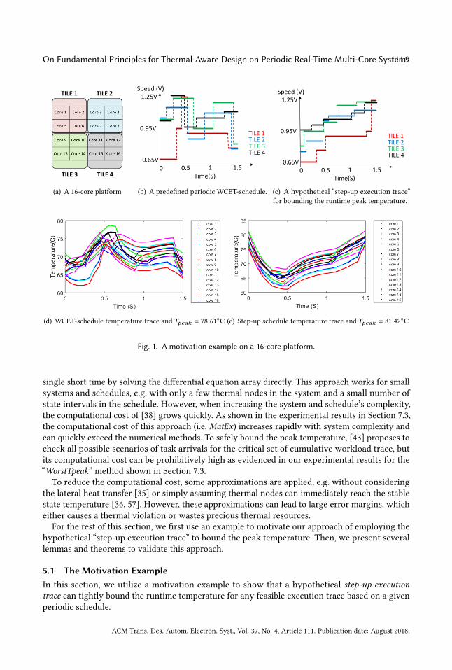
Fig. 1. A motivation example on a 16-core platform.
single short time by solving the differential equation array directly. This approach works for small
systems and schedules, e.g. with only a few thermal nodes in the system and a small number of
state intervals in the schedule. However, when increasing the system and schedule’s complexity,
the computational cost of [38] grows quickly. As shown in the experimental results in Section 7.3,
the computational cost of this approach (i.e. MatEx) increases rapidly with system complexity and
can quickly exceed the numerical methods. To safely bound the peak temperature, [43] proposes to
check all possible scenarios of task arrivals for the critical set of cumulative workload trace, but
its computational cost can be prohibitively high as evidenced in our experimental results for the
“WorstTpeak” method shown in Section 7.3.
To reduce the computational cost, some approximations are applied, e.g. without considering
the lateral heat transfer [35] or simply assuming thermal nodes can immediately reach the stable
state temperature [36, 57]. However, these approximations can lead to large error margins, which
either causes a thermal violation or wastes precious thermal resources.
For the rest of this section, we first use an example to motivate our approach of employing the
hypothetical “step-up execution trace” to bound the peak temperature. Then, we present several
lemmas and theorems to validate this approach.
5.1 The Motivation ExampleIn this section, we utilize a motivation example to show that a hypothetical step-up executiontrace can tightly bound the runtime temperature for any feasible execution trace based on a given
periodic schedule.
ACM Trans. Des. Autom. Electron. Syst., Vol. 37, No. 4, Article 111. Publication date: August 2018.
111:10 Sha and Bankar, et al.
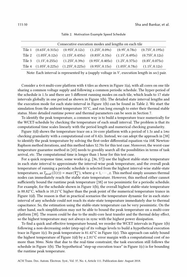
Table 2. Motivation Example Speed Schedule
Consecutive execution modes and lengths on each tile
Tile 1 (0.65𝑉 , 0.315𝑠) (0.95𝑉 , 0.12𝑠) (1.25𝑉 , 0.09𝑠) (0.9𝑉 , 0.78𝑠) (0.75𝑉 , 0.195𝑠)Tile 2 (1.05𝑉 , 0.12𝑠) (1.15𝑉 , 0.435𝑠) (0.85𝑉 , 0.33𝑠) (1.1𝑉 , 0.495𝑠) (0.75𝑉 , 0.12𝑠)Tile 3 (1.1𝑉 , 0.255𝑠) (1.25𝑉 , 0.39𝑠) (0.95𝑉 , 0.405𝑠) (1.2𝑉 , 0.375𝑠) (0.8𝑉 , 0.075𝑠)Tile 4 (1.05𝑉 , 0.225𝑠) (1.25𝑉 , 0.225𝑠) (0.95𝑉 , 0.15𝑠) (1.05𝑉 , 0.78𝑠) (1.1𝑉 , 0.12𝑠)Note: Each interval is represented by a (supply voltage in 𝑉 , execution length in 𝑠𝑒𝑐) pair.
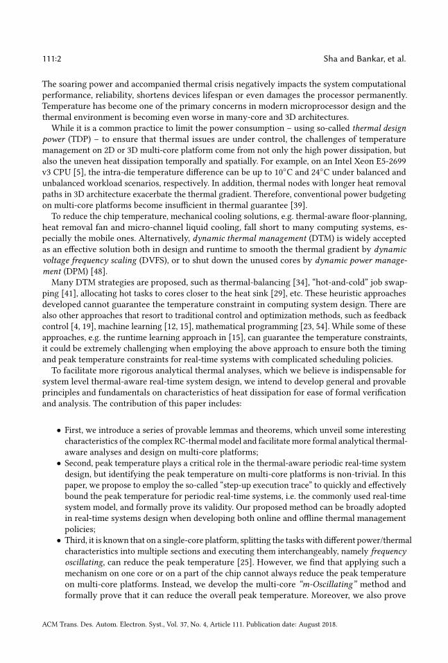
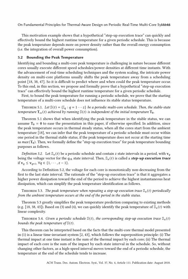
Consider a 4×4 multi-core platform with 4 tiles as shown in Figure 1(a), with all cores on one tile
sharing a common voltage supply and following a common periodic schedule. The hyper-period of
the schedule is 1.5𝑠 and there are 5 different running modes on each tile, which leads to 17 state
intervals globally in one period as shown in Figure 1(b). The detailed state interval lengths and
the execution mode for each state-interval in Figure 1(b) can be found in Table 2. We start the
simulation from the ambient temperature 35C, and run long enough to enter their thermal stable
status. More detailed runtime power and thermal parameters can be seen in Section 7.
To identify the peak temperature, a common way is to build a temperature trace numerically for
the WCET-schedule by checking the temperature of each small interval. The problem is that its
computational time scales linearly with the period length and numerical checking granularity.
Figure 1(d) shows the temperature trace on a 16-core platform with a period of 1.5𝑠 and a 1𝑚𝑠
checking granularity with a computational cost of 0.42𝑠 . Instead, we can adopt the approach in [38]
to identify the peak temperature by solving the first-order differential equation via 10𝐾 Newton-
Raphson method iterations, and this method takes 52.70𝑠 for this test case. Moreover, the worst-case
temperature guarantee method in [43] needs to greedily search all the possibilities in terms of task
arrival, etc. The computational time is longer than 1 hour for this test case.
For a quick response time, some works (e.g. [36, 57]) use the highest stable-state temperature
in each state interval to approximate the interval-wise peak temperature, and the overall peak
temperature of running a periodic schedule is selected from the highest interval-wise stable-state
temperatures, as𝑇𝑝𝑒𝑎𝑘 (S(𝑡)) =𝑚𝑎𝑥 (T∞𝑞 ), where 𝑞 = 1, · · · , 𝑧. This method simply assumes thermal
nodes can immediately reach the stable state temperature. However, this method either cannot
sufficiently bound the runtime peak temperature [38] or too pessimistic for a periodic schedule.
For example, for the schedule shown in Figure 1(b), the overall highest stable-state temperature
is 88.82C, which is 10.21C higher than the peak point of the numerical temperature trance in
Figure 1(d). The reason is that in practical scenarios the temperature dynamic for in each state-
interval of any schedule could not reach its state-state temperature immediately due to thermal
capacitance. So, the estimation using the stable-state temperature can be very pessimistic. On the
other hand, such simplification may not be able to bound the peak temperature on a multi-core
platform [38]. The reason could be due to the multi-core heat transfer and the thermal delay effect,
so the highest temperature may not always in sync with the highest power dissipation.
To find a quick and effective temperature bound, we reorder the WCET intervals in Figure 1(b)
following a non-decreasing order (step-up) of its voltage levels to build a hypothetical execution
trace in Figure 1(c). Its peak temperature is 81.42C in Figure 1(e). This approach can safely bound
the highest temperature of Figure 1(d) by a 2.81C error margin with a computational cost of no
more than 30𝑚𝑠 . Note that due to the real-time constraint, the task execution still follows the
schedule in Figure 1(b). The hypothetical “step-up execution trace” in Figure 1(c) is for bounding
the runtime peak temperature.
ACM Trans. Des. Autom. Electron. Syst., Vol. 37, No. 4, Article 111. Publication date: August 2018.
On Fundamental Principles for Thermal-Aware Design on Periodic Real-Time Multi-Core Systems111:11
This motivation example shows that a hypothetical “step-up execution trace” can quickly and
effectively bound the highest runtime temperature for a given periodic schedule. This is because
the peak temperature depends more on power density rather than the overall energy consumption
(i.e. the integration of overall power consumption).
5.2 Bounding the Peak TemperatureIdentifying and bounding a multi-core peak temperature is challenging in nature because different
cores usually execute different speed schedules/power densities at different time instants. With
the advancement of real-time scheduling techniques and the system scaling, the intricate power
density on multi-core platforms usually shifts the peak temperature away from a scheduling
point [18, 38, 47]. So it is difficult to predict where and when could the peak temperature occur.
To this end, in this section, we propose and formally prove that a hypothetical “step-up execution
trace” can effectively bound the highest runtime temperature for a given periodic schedule.
First, to bound the peak temperature for running a periodic schedule, we prove that the starting
temperature of a multi-core schedule does not influence its stable status temperature.
Theorem 5.1. Let S(𝑡) = I𝑞 : 𝑞 = 1 · · · 𝑧 be a periodic multi-core schedule. Then, the stable-statetemperature T𝑠𝑠 (𝑡) achieved by running S(𝑡) is independent of the initial temperature T0.
Theorem 5.1 shows that when identifying the peak temperature in the stable status, we can
assume T0 = 0 to ease the presentation in this paper, if otherwise specified. In addition, since
the peak temperature occurs in thermal steady status, when all the cores start from the ambient
temperature [18], we can infer that the peak temperature of a periodic schedule must occur within
one period in the thermal stable status, if the peak temperature does not occur at the starting time
as𝑚𝑎𝑥 (T0). Then, we formally define the “step-up execution trace” for peak temperature bounding
purposes as follows.
Definition 5.2. Let S𝑢 (𝑡) be a periodic schedule and contain 𝑧 state intervals in a period, with v𝑞being the voltage vector for the 𝑞𝑡ℎ state interval. Then, S𝑢 (𝑡) is called a step-up execution traceif v𝑞 ≤ v𝑞+1, ∀𝑞 ∈ 1, · · · , 𝑧 − 1.
According to Definition 5.2, the voltage for each core is monotonically non-decreasing from the
first to the last state interval. The rationale of the “step-up execution trace” is that it aggregates a
higher power dissipation toward the end of the period to achieve the highest instantaneous heat
dissipation, which can simplify the peak temperature identification as follows.
Theorem 5.3. The peak temperature when repeating a step-up execution trace S𝑢 (𝑡) periodicallyfrom the ambient temperature occurs at the end of the period in the stable status.
Theorem 5.3 greatly simplifies the peak temperature prediction comparing to existing methods
(e.g. [18, 38, 43]). Based on (3) and (4), we can quickly identify the peak temperature of S𝑢 (𝑡) withlinear complexity.
Theorem 5.4. Given a periodic schedule S(𝑡), the corresponding step-up execution trace S𝑢 (𝑡)bounds the peak temperature of S(𝑡).
This theorem can be interpreted based on the facts that the multi-core thermal model presented
in (1) is a linear time-invariant system [2, 43], which follows the superposition principle: (i) The
thermal impact at one time instant is the sum of the thermal impact by each core; (ii) The thermal
impact of each core is the sum of the impact by each state interval in the schedule. So, without
changing other factors, as a high-speed interval moves toward the end of a periodic schedule, the
temperature at the end of the schedule tends to increase.
ACM Trans. Des. Autom. Electron. Syst., Vol. 37, No. 4, Article 111. Publication date: August 2018.
111:12 Sha and Bankar, et al.
Based on Theorem 5.3 and 5.4, given a periodic schedule S(𝑡) and its corresponding step-up
execution trace S𝑢 (𝑡), as long as all tasks’ deadlines can be guaranteed by S(𝑡) and the peak
temperature constraints can be guaranteed by S𝑢 (𝑡), then both the timing and peak temperature
constraints are guaranteed if S(𝑡) is executed periodically.
6 PEAK TEMPERATURE MINIMIZATIONPeak temperature minimization is one of the primary design objectives in the IC industry. Nowadays,
the escalating software complexity can easily make heat generation exceed the capability of thermal
dissipation systems, which are often designed with narrow or even negative margins for cost reason.
In section 5, it has been proved that the runtime peak temperature can be effectively bounded
by using a hypothetical step-up execution trace. In this section, we discuss how to employ the m-Oscillating methods [45] to reduce the peak temperature bound and improve the real-time service
output on a multi-core platform.
The m-Oscillating scheduling method, as introduced in [25] for a single-processor platform,
frequently changes processor running modes between high and low voltage settings, while keeping
the same workload within the same period to reduce the peak temperature. In what follows, we
show that simply applying the m-Oscillating scheduling method for an individual core or part of
cores on a multicore platform cannot always reduce the peak temperature.
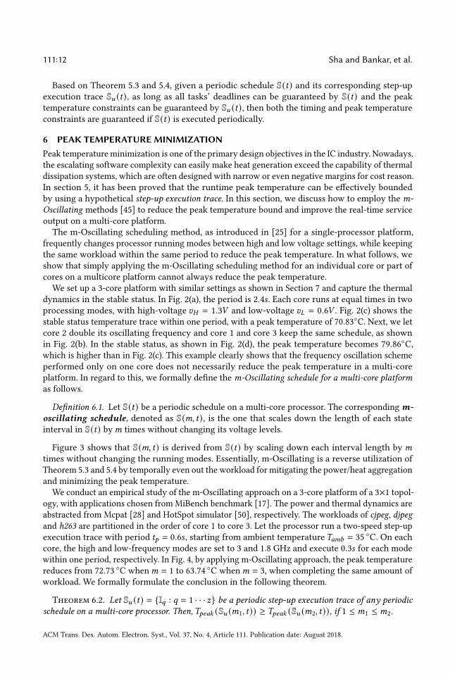
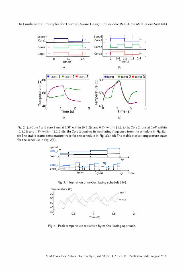
We set up a 3-core platform with similar settings as shown in Section 7 and capture the thermal
dynamics in the stable status. In Fig. 2(a), the period is 2.4𝑠 . Each core runs at equal times in two
processing modes, with high-voltage 𝑣𝐻 = 1.3𝑉 and low-voltage 𝑣𝐿 = 0.6𝑉 . Fig. 2(c) shows the
stable status temperature trace within one period, with a peak temperature of 70.83C. Next, we letcore 2 double its oscillating frequency and core 1 and core 3 keep the same schedule, as shown
in Fig. 2(b). In the stable status, as shown in Fig. 2(d), the peak temperature becomes 79.86C,which is higher than in Fig. 2(c). This example clearly shows that the frequency oscillation scheme
performed only on one core does not necessarily reduce the peak temperature in a multi-core
platform. In regard to this, we formally define the m-Oscillating schedule for a multi-core platformas follows.
Definition 6.1. Let S(𝑡) be a periodic schedule on a multi-core processor. The correspondingm-oscillating schedule, denoted as S(𝑚, 𝑡), is the one that scales down the length of each state
interval in S(𝑡) by𝑚 times without changing its voltage levels.
Figure 3 shows that S(𝑚, 𝑡) is derived from S(𝑡) by scaling down each interval length by 𝑚
times without changing the running modes. Essentially, m-Oscillating is a reverse utilization of
Theorem 5.3 and 5.4 by temporally even out the workload for mitigating the power/heat aggregation
and minimizing the peak temperature.
We conduct an empirical study of the m-Oscillating approach on a 3-core platform of a 3×1 topol-ogy, with applications chosen from MiBench benchmark [17]. The power and thermal dynamics are
abstracted from Mcpat [28] and HotSpot simulator [50], respectively. The workloads of cjpeg, djpegand h263 are partitioned in the order of core 1 to core 3. Let the processor run a two-speed step-up
execution trace with period 𝑡𝑝 = 0.6𝑠 , starting from ambient temperature 𝑇𝑎𝑚𝑏 = 35C. On each
core, the high and low-frequency modes are set to 3 and 1.8 GHz and execute 0.3𝑠 for each mode
within one period, respectively. In Fig. 4, by applying m-Oscillating approach, the peak temperature
reduces from 72.73 C when𝑚 = 1 to 63.74
C when𝑚 = 3, when completing the same amount of
workload. We formally formulate the conclusion in the following theorem.
Theorem 6.2. Let S𝑢 (𝑡) = I𝑞 : 𝑞 = 1 · · · 𝑧 be a periodic step-up execution trace of any periodicschedule on a multi-core processor. Then, 𝑇𝑝𝑒𝑎𝑘 (S𝑢 (𝑚1, 𝑡)) ≥ 𝑇𝑝𝑒𝑎𝑘 (S𝑢 (𝑚2, 𝑡)), if 1 ≤ 𝑚1 ≤ 𝑚2.
ACM Trans. Des. Autom. Electron. Syst., Vol. 37, No. 4, Article 111. Publication date: August 2018.
On Fundamental Principles for Thermal-Aware Design on Periodic Real-Time Multi-Core Systems111:13
…Core1
Core2
1.20 2.4
…
…
…
Speed
Time(s)
…
Core3
…
(a)
…Core1
Core2
1.20 2.4
…
…
…
Speed
Time(s)
…
Core3
…
0.6 1.8
(b)
0 1 2 340
60
80
Time (s)
Tem
pera
ture
(C)
core 1 core 2 core 3
Student Version of MATLAB
(c)
0 1 2 340
60
80
Time (s)
Tem
pera
ture
(C)
core 1 core 2 core 3
Student Version of MATLAB
(d)
Fig. 2. (a) Core 1 and core 3 run at 1.3𝑉 within [0, 1.2]𝑠 and 0.6𝑉 within [1.2, 2.4]𝑠 ; Core 2 runs at 0.6𝑉 within[0, 1.2]𝑠 and 1.3𝑉 within [1.2, 2.4]𝑠 . (b) Core 2 doubles its oscillating frequency from the schedule in Fig.2(a).(c) The stable status temperature trace for the schedule in Fig. 2(a). (d) The stable status temperature tracefor the schedule in Fig. 2(b).
tptp/m 2tp/m
…tp
core_i
core_ jcore_iSpeed
core_ jm
Time
Fig. 3. Illustration of m-Oscillating schedule [46].
0 0.5 1 1.5 23040506070
Student Version of MATLAB
Time (S)
Temperature (C)m=1
m = 3
Fig. 4. Peak temperature reduction by m-Oscillating approach.
ACM Trans. Des. Autom. Electron. Syst., Vol. 37, No. 4, Article 111. Publication date: August 2018.
111:14 Sha and Bankar, et al.
0
t’pt’i,Ht’i,L
ti,LA’
B
servicecapacity
A
bdf (Δ,ρ( A , B ), l( 0 , A ))
bdf (Δ,ρ( A’ , B’ ), l(0 , A’))guaranteed output service of S(m1, t)
guaranteed output service of S(m2,t)
B’
ti,H tptime
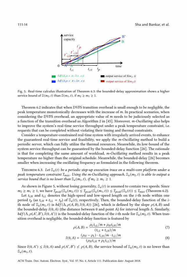
Fig. 5. Real-time calculus illustration of Theorem 6.3: the bounded-delay approximation shows a higherservice bound of S(𝑚2, 𝑡) than S(𝑚1, 𝑡), if𝑚2 ≥ 𝑚1 ≥ 1.
Theorem 6.2 indicates that when DVFS transition overhead is small enough to be negligible, the
peak temperature monotonically decreases with the increase of𝑚. In practical scenarios, when
considering the DVFS overhead, an appropriate value of 𝑚 needs to be judiciously selected as
a function of the transition overhead as Algorithm 2 in [45]. Moreover, m-Oscillating also helps
to improve the system’s real-time service throughput under a peak temperature constraint, i.e.
requests that can be completed without violating their timing and thermal constraints.
Consider a temperature-constrained real-time system with irregularly arrived events, to enhance
the guaranteed real-time service and feasibility, we apply the m-Oscillating method to build a
periodic server, which can fully utilize the thermal resources. Meanwhile, its low-bound of the
system service throughput can be guaranteed by the bounded-delay function [26]. The rationale
is that for completing the same amount of workload, m-Oscillating method results in a peak
temperature no higher than the original schedule. Meanwhile, the bounded-delay [26] becomes
smaller when increasing the oscillating frequency as formulated in the following theorem.
Theorem 6.3. Let S𝑢 (𝑡) be a periodic step-up execution trace on a multi-core platform under apeak temperature constraint 𝑇𝑚𝑎𝑥 . Using the m-Oscillating approach, S𝑢 (𝑚2, 𝑡) is able to output aservice bound that is no lower than S𝑢 (𝑚1, 𝑡), if𝑚2 ≥ 𝑚1 ≥ 1.
As shown in Figure 5, without losing generality, S𝑢 (𝑡) is assumed to contain two speeds. Since
𝑚2 ≥ 𝑚1 ≥ 1, we have 𝑇𝑝𝑒𝑎𝑘 (S𝑢 (𝑚2, 𝑡)) ≤ 𝑇𝑝𝑒𝑎𝑘 (S𝑢 (𝑚1, 𝑡)) ≤ 𝑇𝑝𝑒𝑎𝑘 (S𝑢 (𝑡)) ≤ 𝑇𝑚𝑎𝑥 (Theorem 6.2).
Let 𝑡𝑖,𝐻 and 𝑡𝑖,𝐿 denotes the high-speed and low-speed length on the 𝑖-th node within one
period 𝑡𝑝 (as 𝑡𝑖,𝐻 + 𝑡𝑖,𝐿 = 𝑡𝑝 ) of S𝑢 (𝑡), respectively. Then, the bounded-delay function of the 𝑖-
th node of S𝑢 (𝑚1, 𝑡) is 𝑏𝑑 𝑓 (Δ, 𝜌 (𝐴, 𝐵), 𝑙 (0, 𝐴)) [26], which is defined by the slope 𝜌 (𝐴, 𝐵) andthe bounded-delay 𝑙 (0, 𝐴) (the distance between 0 and point A) for interval length Δ. Similarly,
𝑏𝑑 𝑓 (Δ, 𝜌 (𝐴′, 𝐵′), 𝑙 (0, 𝐴′)) is the bounded-delay function of the 𝑖-th node for S𝑢 (𝑚2, 𝑡). When tran-
sition overhead is negligible, the bounded-delay function is featured by
𝜌 (𝐴, 𝐵) = 𝜌𝐿𝑡𝑖,𝐿/𝑚 + 𝜌𝐻 𝑡𝑖,𝐻/𝑚(𝑡𝑖,𝐿 + 𝑡𝑖,𝐻 )/𝑚
(7)
𝑙 (0, 𝐴) = (𝜌𝐻 − 𝜌𝐿) · 𝑡𝑖,𝐻/𝑚 · 𝑡𝑖,𝐿/𝑚(𝜌𝐻 𝑡𝑖,𝐻 + 𝜌𝐿𝑡𝑖,𝐿)/𝑚
(8)
Since 𝑙 (0, 𝐴′) ≤ 𝑙 (0, 𝐴) and 𝜌 (𝐴′, 𝐵′) ≮ 𝜌 (𝐴, 𝐵), the service bound of S𝑢 (𝑚2, 𝑡) is no lower than
S𝑢 (𝑚1, 𝑡).
ACM Trans. Des. Autom. Electron. Syst., Vol. 37, No. 4, Article 111. Publication date: August 2018.

On Fundamental Principles for Thermal-Aware Design on Periodic Real-Time Multi-Core Systems111:15
Theorem 6.3 implies that, when using the m-Oscillating approach, the larger the value of𝑚 is,
the higher the server capacity becomes. However, this conclusion is built upon the assumption that
the execution mode transition overhead is small and can be ignored.
When transition overhead is significant, service rates for 𝑆𝑢 (𝑚1, 𝑡) and 𝑆𝑢 (𝑚2, 𝑡) are differentwhen they adopt the same running mode. Therefore, increasing𝑚 does not necessarily always lead
to improved real-time service bound.
Let 𝜏 be the transition overhead on the given platform and let 𝑏𝑑 𝑓 (Δ, 𝜌 (, , 𝜏), 𝑙 (0, , 𝜏)) be thebounded-delay function of the 𝑖-th node of S𝑢 (𝑚, 𝑡) when considering the transition overhead 𝜏 . To
construct the m-Oscillating schedule, we need to compensate for the performance loss caused by
each DVFS transition stalls, i.e. (𝜌𝐻 + 𝜌𝐿)𝜏 . So, a small interval of 𝛿 =(𝜌𝐻 +𝜌𝐿)𝜏𝜌𝐻−𝜌𝐿 needs to be shifted
from low-speed to high-speed (as shown in [46] Figure 6a). To maximize the system performances,
we first find the “optimal m", which leads to the lowest peak temperature for a given schedule.
Then, we judiciously increase the high-speed interval lengths until approaching the maximally
allowed temperature [46]. When considering transition overhead, the bounded-delay function is
featured by
𝜌 (, , 𝜏) = 𝜌𝐿 (𝑡𝑖,𝐿/𝑚 − 𝛿) + 𝜌𝐻 (𝑡𝑖,𝐻/𝑚 + 𝛿)(𝑡𝑖,𝐿 + 𝑡𝑖,𝐻 )/𝑚 + 2𝜏
, (9)
and
𝑙 (0, , 𝜏) = 𝜌𝐻 (𝑡𝑖,𝐻/𝑚 + 𝛿) (𝑡𝑖,𝐿/𝑚 + 𝜏 − 𝛿) − 𝜌𝐿 (𝑡𝑖,𝐿/𝑚 − 𝛿) (𝑡𝑖,𝐻/𝑚 + 𝜏 + 𝛿)𝜌𝐿 (𝑡𝑖,𝐿/𝑚 − 𝛿) + 𝜌𝐻 (𝑡𝑖,𝐻/𝑚 + 𝛿) . (10)
In what follows, we conduct an empirical study under the same power and thermal configurations
as shown in Section 7. To validate Theorem 6.3, we set a two-speed schedule whose low-/high-
speeds are supported by 0.6𝑉 and 1.3𝑉 , respectively. The maximally allowed temperature is set to
70C. The period is 1.5𝑠𝑒𝑐 and high-/low- speed takes 80% and 20% of the period length without
considering overhead, respectively. Then, we incorporate DVFS transition overhead and conduct
m-Oscillating approach (Algorithm 2 in [45]). The system throughput is defined as the average
speed within one period, which is defined in Equation 5 of [45].
0.950.960.970.980.99
11.011.021.03
0 100 200 300 400 500 600
throughtput rho
rho andthroughput (V)
throughputm
(a) 𝜌 ( ˜(𝐴), , 𝜏) and throughput (V)
0
0.005
0.01
0.015
0.02
0.025
0.03
0 100 200 300 400 500 600
delay l
m
(b) 𝑙 (0, , 𝜏)
Fig. 6. Results for bounded-delay approximation when considering DVFS overhead
From Figure 6(a), we can see that the throughput performance is monotonically increasing
with𝑚 first and the maximal throughput is achieved when𝑚 = 161. Meanwhile, factor 𝜌 (, , 𝜏)in (9) reaches its maximum value. Then, both throughput and factor 𝜌 (, , 𝜏) decrease with𝑚.
ACM Trans. Des. Autom. Electron. Syst., Vol. 37, No. 4, Article 111. Publication date: August 2018.

111:16 Sha and Bankar, et al.
From Figure 6(b), we can see that 𝑙 (0, , 𝜏) in (10) monotonically decreases with𝑚. Overall, when
incorporating transition overhead, the m-Oscillating approach is able to output the maximum
service bound.
7 EXPERIMENTAL RESULTSIn this section, we focus on simulating a series of peak temperature bounding methodologies on 4
multi-core configurations, i.e. 2×3, 3×3, 3×4 and 4×4 corresponding to 6, 9, 12, 16-core, respectively.Each core size is 4 × 4𝑚𝑚2
and follows the Alpha 21264 floorplan and there are fifteen available
speed levels supported by discrete supply voltages from 0.6𝑉 to 1.3𝑉 with a 0.05𝑉 step-length.
The thermal and power parameters are abstracted from HotSpot 5.02 [27] and the McPAT
simulator [28]. The total power consumption (𝑃) is composed of dynamic power and leakage
power. Dynamic power is proportional to the cubic of supply voltage and leakage power depends
linearly on temperature 𝑇 as 𝑃𝑙𝑒𝑎𝑘 = 𝛼 (𝑣) + 𝛽𝑇 (𝑡). The total power of the ^-th core is 𝑃^ (𝑡) =
𝛼 (𝑣^) + 𝛽𝑇^ (𝑡) + 𝛾 (𝑣^)𝑣3^ , where 𝛼 and 𝛾 are positive constants within the interval that 𝑐𝑜𝑟𝑒^ runs
at supply voltage 𝑣^ . 𝛽 is a constant. In particular, we adopt the curve-fitting constants [18] in the
power model as: 1) 𝛼 = 0.84; 2) 𝛽 = 0.0163; and 3) 𝛾 = 7.2564. The ambient temperature was set
to be 𝑇𝑎𝑚𝑏 = 35C, unless otherwise specified. In this paper, we assume the WCET-schedules are
given, so there should be free of any deadline miss case.
There are five approaches in this experiment: (1) Numerical method (NM) splits each exe-
cution interval into small pieces and finds the peak temperature by checking each small step
length (e.g. [40, 47, 50]). (2) Stable State Temperature Check method (TssCheck) checks the
peak temperature interval-by-interval using a combination of the analytical and numerical ap-
proaches [18]. (3) Maximum Transient Temperature approach (MatEx) uses Newton-Raphsonmethod to solve the first-order derivative on each core in (1) as shown in [38]. (4) Worst-Case
Temperature Guarantees method (WorstTpeak) uses an analytical method to calculate the upper
bound via building the thermal critical instance under all possible scenarios of task executions
in [43]. (5) The last one is our proposed method, i.e. constructing a step-up execution trace (StepUp)to bound the peak temperature of different runtime execution traces, as defined in Definition 5.2.
In the following experiments, the checking step length used inNM, TssCheck andWorstTpeakare set as 1𝑚𝑠 , and the number of iterations used when applying the Newton-Raphson method
by MatEx is set as 10𝐾 , unless otherwise specified.
7.1 The step-up execution trace can bound the peak temperatureFirst, we utilize random schedules to validate that a hypothetical step-up execution trace can
effectively bound predefinedWCET-schedule. To put the runtime thermal dynamics into perspective,
we select a 3-core worst-case execution time schedule with a period of 3 seconds given in Figure 7(a).
Core 1 runs at the mode with the supply voltage of 1.5𝑉 for 1.26𝑠 , then turns to 0.9𝑉 for 0.36𝑠 and
executes at 1.5𝑉 again for 1.38𝑠 . Core 2 runs at 1.05𝑉 for 0.9𝑠 , then turns to 1.0𝑉 for 1.17𝑠 and
executes at 1.1𝑉 for 0.93𝑠 . Core 3 runs at 0.65𝑉 for 0.54𝑠 , then turns to 1.3𝑉 for 1.44𝑠 and executes
at 0.7𝑉 for 1.02𝑠 .
Figure 7(b) shows that the peak temperature for executing the schedule in Figure 7(a) is 68.2907C.If we reorder the WCET intervals in Figure 7(a) following the step-up execution trace (in Defini-
tion 5.2) as shown in Figure 7(c), the peak temperature is calculated as 68.8824C in Figure 7(d),
which is higher than the peak temperature in Figure 7(b) (conform to Theorem 5.4). In addition,
the peak temperature of a step-up execution trace occurs at the end of the period in Figure 7(d)
(conform to Theorem 5.3). We also profiled the temperature trace in the thermal stable status on 6,
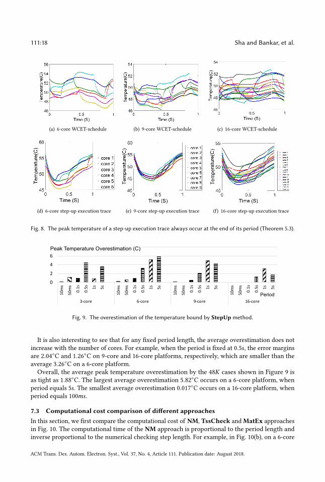
9 and 16-core architectures as shown in Figure 8. We can observe that all the peak temperatures in
the step-up execution trace must occur at the end of the period, which conforms to Theorem 5.3.
ACM Trans. Des. Autom. Electron. Syst., Vol. 37, No. 4, Article 111. Publication date: August 2018.

On Fundamental Principles for Thermal-Aware Design on Periodic Real-Time Multi-Core Systems111:17
0 1 2 3
Speed (V)
Time(S)0.65V
1.05V
1.30VCORE 1
CORE 2
CORE 3
(a) A predefined periodic WCET-schedule. (b) 𝑇𝑝𝑒𝑎𝑘 = 68.2907C
0 1 2 3
Speed (V)
Time(S)0.65V
1.05V
1.30VCORE 1
CORE 2
CORE 3
(c) A hypothetical “step-up execution trace”
for bounding the runtime peak temperature.
(d) 𝑇𝑝𝑒𝑎𝑘 = 68.8824C
Fig. 7. An illustration of Theorem 5.3 on a 3-core platform.
Meanwhile, we can also observe that the peak temperature of the step-up execution trace must be
higher than WCET-schedule, which conforms to Theorem 5.4. More intensive experiments are
shown in what follows regarding how effectively can a step-up execution trace bound the peak
temperature.
7.2 The tightness of the temperature bound by StepUp methodIn this section, we arbitrarily generate randomWCET-schedules for each configuration by a different
number of cores and different period lengths. Each schedule may contain up to 20 state intervals.
Then, we use the peak temperature differences between the step-up execution traces and WCET-
schedules to represent the bounding tightness of the StepUp methodology. In Figure 9, each bar
represents the average peak temperature overestimation for 2𝐾 random WCET-schedules under a
given configuration.
In general, the peak temperature overestimation is proportional to the period length. For example
in Figure 9, on a 6-core platform, the overestimation is 0.17C, 0.60C and 0.85C for the periods
equal to 10𝑚𝑠 , 50𝑚𝑠 and 100𝑚𝑠 , respectively. As the period becomes 0.5𝑠 , 1𝑠 and 5𝑠 , the overestima-
tion shows 3.26C, 5.22C and 5.82C, respectively, which has significantly larger margins than
those cases with smaller period lengths. The reason is that the larger the period, the more likely
those high-speed intervals may stack longer to the end of the period, and, thus, causes a higher
peak temperature in the hypothetical step-up schedule.
However, for 3-core, 9-core and 16-core cases, the overestimation may not strictly increase with
the period length. For example, on the 16-core platform, the overestimation is 1.73C when the
period equals 5𝑠 , which is smaller than 3.12C when the period equals 1𝑠 . The reason can be that
although the randomly generated WCET-schedules exhibit intricate power dissipation and heat
transfer, its corresponding hypothetical step-up schedule may not always significantly worsen the
power aggregation as periods become larger.
ACM Trans. Des. Autom. Electron. Syst., Vol. 37, No. 4, Article 111. Publication date: August 2018.
111:18 Sha and Bankar, et al.
(a) 6-core WCET-schedule (b) 9-core WCET-schedule (c) 16-core WCET-schedule
(d) 6-core step-up execution trace (e) 9-core step-up execution trace (f) 16-core step-up execution trace
Fig. 8. The peak temperature of a step-up execution trace always occur at the end of its period (Theorem 5.3).
0
2
4
6
8
10ms
50ms
0.1s
0.5s 1s 5s
10ms
50ms
0.1s
0.5s 1s 5s
10ms
50ms
0.1s
0.5s 1s 5s
10ms
50ms
0.1s
0.5s 1s 5s
3-core 6-core 9-core 16-core
Peak Temperature Overestimation (C)
Period Period
Fig. 9. The overestimation of the temperature bound by StepUp method.
It is also interesting to see that for any fixed period length, the average overestimation does not
increase with the number of cores. For example, when the period is fixed at 0.5𝑠 , the error margins
are 2.04C and 1.26C on 9-core and 16-core platforms, respectively, which are smaller than the
average 3.26C on a 6-core platform.
Overall, the average peak temperature overestimation by the 48𝐾 cases shown in Figure 9 is
as tight as 1.88C. The largest average overestimation 5.82C occurs on a 6-core platform, when
period equals 5𝑠 . The smallest average overestimation 0.017C occurs on a 16-core platform, when
period equals 100𝑚𝑠 .
7.3 Computational cost comparison of different approachesIn this section, we first compare the computational cost of NM, TssCheck andMatEx approaches
in Fig. 10. The computational time of the NM approach is proportional to the period length and
inverse proportional to the numerical checking step length. For example, in Fig. 10(b), on a 6-core
ACM Trans. Des. Autom. Electron. Syst., Vol. 37, No. 4, Article 111. Publication date: August 2018.
On Fundamental Principles for Thermal-Aware Design on Periodic Real-Time Multi-Core Systems111:19
0123
1 3 5 10 1 3 5 10 1 3 5 10
2-interval 3-interval 5-interval
Computational Cost (s)
Period(s)
(a) 3-core platform
0123
1 3 5 10 1 3 5 10 1 3 5 10
2-interval 3-interval 5-interval
Computational Cost (s)
Period(s)
(b) 6-core platform
01234
1 3 5 10 1 3 5 10 1 3 5 10
2-interval 3-interval 5-interval
NM TssCheck MatEx
Computational Cost (s)
Period(s)
(c) 9-core platform
0
20
40
60
1 3 5 10 1 3 5 10 1 3 5 10
2-interval 3-interval 5-interval
NM TssCheck MatEx
Computational Cost (s)
Period(s)
(d) 16-core platform
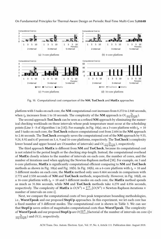
Fig. 10. Computational cost comparison of the NM, TssCheck and MatEx approaches
platformwith 5 tasks on each core, theNM computational cost increases from 0.272 to 2.848 seconds,
when 𝑡𝑝 increases from 1 to 10 seconds. The complexity of the NM approach is 𝑂 ( 𝑡𝑝
step length).
The second approach TssCheck can be seen as a refinedNM approach by eliminating the numer-
ical checking workloads on those intervals whose peak temperature must occur at the scheduling
points (Line 3 - 8 of Algorithm 1 in [18]). For example, in Fig. 10(a), on a 3-core platform with 𝑡𝑝 = 10
and 5 tasks on each core, the TssCheck reduces computational cost from 2.604 in theNM approach
to 2.46 seconds. The TssCheck averagely saves the computational cost of theNM approach by 9.55,
9.24, 8.92 and 6.47 percent on 3, 6, 9 and 16-core platforms, respectively. TheTssCheck’s complexity
lower bound and upper bound are 𝑂 (number of intervals) and 𝑂 ( 𝑡𝑝
step length), respectively.
The third approach MatEx is different from NM and TssCheck, because its computational cost
is not related to the period length or the checking step-length. Instead, the computational overhead
of MatEx closely relates to the number of intervals on each core, the number of cores, and the
number of iterations used when applying the Newton-Raphson method [38]. For example, on 3 and
6-core platforms, MatEx is significantly computational efficient comparing to NM and TssCheckmethods as shown in Fig. 10(a) and Fig. 10(b). In Fig. 10(b), on a 6-core platform with 𝑡𝑝 = 10 and
3 different modes on each core, the MatEx method only uses 0.464 seconds in comparison with
2.772 and 2.558 seconds of NM and TssCheck methods, respectively. However, in Fig. 10(d), on
a 16-core platform with 𝑡𝑝 = 10 and 3 different modes on each core, the MatEx method spends
as much as 31.866 seconds, while NM and TssCheck methods take 4.270 and 4.056 seconds,
respectively. The complexity of MatEx is 𝑂 (𝑁 3) +∑𝑁𝑖=1 [𝑂 (𝑁 2) × Newton-Raphson iterations ×
number of intervals on core i].
Next, we compare the computational costs of two peak temperature bounding methodologies,
i.e., WorstTpeak and our proposed StepUp approaches. In this experiment, we let each core has
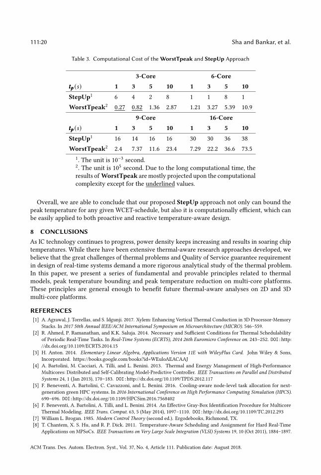
a fixed number of 3 different modes. The computational cost is shown in Table 3. We can see
that StepUp saves orders of magnitudes computational costs than WorstTpeak. The complexity
of WorstTpeak and our proposed StepUp are𝑂 (∏𝑁𝑖=1 [factorial of the number of intervals on core-i]×
𝑡𝑝
step length) and 𝑂 (1), respectively.
ACM Trans. Des. Autom. Electron. Syst., Vol. 37, No. 4, Article 111. Publication date: August 2018.
111:20 Sha and Bankar, et al.
Table 3. Computational Cost of theWorstTpeak and StepUp Approach
3-Core 6-Core𝑡𝑝𝑡𝑝𝑡𝑝 (𝑠) 1 3 5 10 1 3 5 10
StepUp1 6 4 2 8 1 1 8 1
WorstTpeak20.27 0.82 1.36 2.87 1.21 3.27 5.39 10.9
9-Core 16-Core𝑡𝑝𝑡𝑝𝑡𝑝 (𝑠) 1 3 5 10 1 3 5 10
StepUp1 16 14 16 16 30 30 36 38
WorstTpeak22.4 7.37 11.6 23.4 7.29 22.2 36.6 73.5
1. The unit is 10
−3second.
2. The unit is 10
5second. Due to the long computational time, the
results of WorstTpeak are mostly projected upon the computational
complexity except for the underlined values.
Overall, we are able to conclude that our proposed StepUp approach not only can bound the
peak temperature for any given WCET-schedule, but also it is computationally efficient, which can
be easily applied to both proactive and reactive temperature-aware design.
8 CONCLUSIONSAs IC technology continues to progress, power density keeps increasing and results in soaring chip
temperatures. While there have been extensive thermal-aware research approaches developed, we
believe that the great challenges of thermal problems and Quality of Service guarantee requirement
in design of real-time systems demand a more rigorous analytical study of the thermal problem.
In this paper, we present a series of fundamental and provable principles related to thermal
models, peak temperature bounding and peak temperature reduction on multi-core platforms.
These principles are general enough to benefit future thermal-aware analyses on 2D and 3D
multi-core platforms.
REFERENCES[1] A. Agrawal, J. Torrellas, and S. Idgunji. 2017. Xylem: Enhancing Vertical Thermal Conduction in 3D Processor-Memory
Stacks. In 2017 50th Annual IEEE/ACM International Symposium on Microarchitecture (MICRO). 546–559.[2] R. Ahmed, P. Ramanathan, and K.K. Saluja. 2014. Necessary and Sufficient Conditions for Thermal Schedulability
of Periodic Real-Time Tasks. In Real-Time Systems (ECRTS), 2014 26th Euromicro Conference on. 243–252. DOI:http://dx.doi.org/10.1109/ECRTS.2014.15
[3] H. Anton. 2014. Elementary Linear Algebra, Applications Version 11E with WileyPlus Card. John Wiley & Sons,
Incorporated. https://books.google.com/books?id=WEuloAEACAAJ
[4] A. Bartolini, M. Cacciari, A. Tilli, and L. Benini. 2013. Thermal and Energy Management of High-Performance
Multicores: Distributed and Self-Calibrating Model-Predictive Controller. IEEE Transactions on Parallel and DistributedSystems 24, 1 (Jan 2013), 170–183. DOI:http://dx.doi.org/10.1109/TPDS.2012.117
[5] F. Beneventi, A. Bartolini, C. Cavazzoni, and L. Benini. 2016. Cooling-aware node-level task allocation for next-
generation green HPC systems. In 2016 International Conference on High Performance Computing Simulation (HPCS).690–696. DOI:http://dx.doi.org/10.1109/HPCSim.2016.7568402
[6] F. Beneventi, A. Bartolini, A. Tilli, and L. Benini. 2014. An Effective Gray-Box Identification Procedure for Multicore
Thermal Modeling. IEEE Trans. Comput. 63, 5 (May 2014), 1097–1110. DOI:http://dx.doi.org/10.1109/TC.2012.293[7] William L. Brogan. 1985. Modern Control Theory (second ed.). Ergodebooks, Richmond, TX.
[8] T. Chantem, X. S. Hu, and R. P. Dick. 2011. Temperature-Aware Scheduling and Assignment for Hard Real-Time
Applications on MPSoCs. IEEE Transactions on Very Large Scale Integration (VLSI) Systems 19, 10 (Oct 2011), 1884–1897.
ACM Trans. Des. Autom. Electron. Syst., Vol. 37, No. 4, Article 111. Publication date: August 2018.
On Fundamental Principles for Thermal-Aware Design on Periodic Real-Time Multi-Core Systems111:21
DOI:http://dx.doi.org/10.1109/TVLSI.2010.2058873[9] Vivek Chaturvedi, Huang Huang, Shangping Ren, and Gang Quan. 2012. On the Fundamentals of Leakage Aware
Real-time DVS Scheduling for Peak Temperature Minimization. J. Syst. Archit. 58, 10 (Nov. 2012), 387–397. DOI:http://dx.doi.org/10.1016/j.sysarc.2012.08.002
[10] Y. Chen, E. Kursun, D. Motschman, C. Johnson, and Y. Xie. 2011. Analysis and mitigation of lateral thermal blockage
effect of through-silicon-via in 3D IC designs. In IEEE/ACM International Symposium on Low Power Electronics andDesign. 397–402. DOI:http://dx.doi.org/10.1109/ISLPED.2011.5993673
[11] A. K. Coskun, J. L. Ayala, D. Atienza, T. S. Rosing, and Y. Leblebici. 2009. Dynamic thermal management in 3D
multicore architectures. In 2009 Design, Automation Test in Europe Conference Exhibition. 1410–1415. DOI:http://dx.doi.org/10.1109/DATE.2009.5090885
[12] A. Das, R. A. Shafik, G. V. Merrett, B. M. Al-Hashimi, A. Kumar, and B. Veeravalli. 2014. Reinforcement learning-
based inter- and intra-application thermal optimization for lifetime improvement of multicore systems. In 2014 51stACM/EDAC/IEEE Design Automation Conference (DAC). 1–6. DOI:http://dx.doi.org/10.1145/2593069.2593199
[13] Songchun Fan, Seyed Majid Zahedi, and Benjamin C. Lee. 2016. The Computational Sprinting Game. SIGOPS Oper.Syst. Rev. 50, 2 (March 2016), 561–575. DOI:http://dx.doi.org/10.1145/2954680.2872383
[14] Nathan Fisher, Jian-Jia Chen, Shengquan Wang, and Lothar Thiele. 2011. Thermal-aware Global Real-time Scheduling
and Analysis on Multicore Systems. J. Syst. Archit. 57, 5 (May 2011), 547–560. DOI:http://dx.doi.org/10.1016/j.sysarc.2010.09.010
[15] Y. Ge and Q. Qiu. 2011. Dynamic thermal management for multimedia applications using machine learning. In DesignAutomation Conference (DAC), 2011 48th ACM/EDAC/IEEE. 95–100.
[16] C. E. Green, A. G. Fedorov, and Y. K. Joshi. 2012. Dynamic thermal management of high heat flux devices using
embedded solid-liquid phase change materials and solid state coolers. In 13th InterSociety Conference on Thermal andThermomechanical Phenomena in Electronic Systems. 853–862.
[17] M. R. Guthaus, J. S. Ringenberg, D. Ernst, T. M. Austin, T. Mudge, and R. B. Brown. 2001. MiBench: A free, commercially
representative embedded benchmark suite. In Proceedings of the Fourth Annual IEEE International Workshop onWorkloadCharacterization. WWC-4 (Cat. No.01EX538). 3–14. DOI:http://dx.doi.org/10.1109/WWC.2001.990739
[18] Q. Han, M. Fan, O. Bai, S. Ren, and G. Quan. 2016. Temperature-Constrained Feasibility Analysis for Multi-core
Scheduling. IEEE Transactions on Computer-Aided Design of Integrated Circuits and Systems PP, 99 (2016), 1–1. DOI:http://dx.doi.org/10.1109/TCAD.2016.2543020
[19] Vinay Hanumaiah, Digant Desai, Benjamin Gaudette, Carole-Jean Wu, and Sarma Vrudhula. 2014. STEAM: A Smart
Temperature and Energy Aware Multicore Controller. ACM Trans. Embed. Comput. Syst. 13, 5s, Article 151 (Oct. 2014),25 pages. DOI:http://dx.doi.org/10.1145/2661430
[20] V. Hanumaiah and S. Vrudhula. 2011. Reliability-aware thermal management for hard real-time applications on multi-
core processors. In 2011 Design, Automation Test in Europe. 1–6. DOI:http://dx.doi.org/10.1109/DATE.2011.5763032[21] V. Hanumaiah and S. Vrudhula. 2012. Temperature-Aware DVFS for Hard Real-Time Applications on Multicore
Processors. IEEE Trans. Comput. 61, 10 (Oct 2012), 1484–1494. DOI:http://dx.doi.org/10.1109/TC.2011.156[22] V. Hanumaiah and S. Vrudhula. 2014. Energy-Efficient Operation of Multicore Processors by DVFS, Task Migration,
and Active Cooling. IEEE Trans. Comput. 63, 2 (Feb 2014), 349–360. DOI:http://dx.doi.org/10.1109/TC.2012.213[23] V. Hanumaiah, S. Vrudhula, and K.S. Chatha. 2011. Performance Optimal Online DVFS and Task Migration Techniques
for Thermally Constrained Multi-Core Processors. Computer-Aided Design of Integrated Circuits and Systems, IEEETransactions on 30, 11 (Nov 2011), 1677–1690. DOI:http://dx.doi.org/10.1109/TCAD.2011.2161308
[24] M. Healy, M. Vittes, M. Ekpanyapong, C. S. Ballapuram, S. K. Lim, H. S. Lee, and G. H. Loh. 2007. Multiobjective
Microarchitectural Floorplanning for 2-D and 3-D ICs. IEEE Transactions on Computer-Aided Design of IntegratedCircuits and Systems 26, 1 (Jan 2007), 38–52. DOI:http://dx.doi.org/10.1109/TCAD.2006.883925
[25] Huang Huang, Vivek Chaturvedi, Gang Quan, Jeffrey Fan, and Meikang Qiu. 2014. Throughput Maximization for
Periodic Real-time Systems Under the Maximal Temperature Constraint. ACM Trans. Embed. Comput. Syst. 13, 2s,Article 70 (Jan. 2014), 22 pages. DOI:http://dx.doi.org/10.1145/2544375.2544390
[26] K. Huang, L. Santinelli, J. J. Chen, L. Thiele, and G. C. Buttazzo. 2009. Periodic power management schemes for
real-time event streams. In Proceedings of the 48h IEEE Conference on Decision and Control (CDC) held jointly with 200928th Chinese Control Conference. 6224–6231. DOI:http://dx.doi.org/10.1109/CDC.2009.5400034
[27] Wei Huang, S. Ghosh, S. Velusamy, K. Sankaranarayanan, K. Skadron, and M.R. Stan. 2006. HotSpot: a compact thermal
modeling methodology for early-stage VLSI design. Very Large Scale Integration (VLSI) Systems, IEEE Transactions on14, 5 (May 2006), 501–513. DOI:http://dx.doi.org/10.1109/TVLSI.2006.876103
[28] Sheng Li, Jung Ho Ahn, R.D. Strong, J.B. Brockman, D.M. Tullsen, and N.P. Jouppi. 2009. McPAT: An integrated power,
area, and timing modeling framework for multicore and manycore architectures. In Microarchitecture, 2009. MICRO-42.42nd Annual IEEE/ACM International Symposium on. 469–480.
ACM Trans. Des. Autom. Electron. Syst., Vol. 37, No. 4, Article 111. Publication date: August 2018.
111:22 Sha and Bankar, et al.
[29] C. H. Liao and C. H. P. Wen. 2015. Thermal-Constrained Task Scheduling on 3-D Multicore Processors for Throughput-
and-Energy Optimization. IEEE Transactions on Very Large Scale Integration (VLSI) Systems 23, 11 (Nov 2015), 2719–2723.DOI:http://dx.doi.org/10.1109/TVLSI.2014.2360802
[30] M. Marcus and H. Minc (Eds.). 1964. A Survey of Matrix Theory and Matrix Inequalities. Allyn and Bacon, Boston, MA,
USA.
[31] J. Meng, K. Kawakami, and A. K. Coskun. 2012. Optimizing energy efficiency of 3-D multicore systems with stacked
DRAM under power and thermal constraints. In DAC Design Automation Conference 2012. 648–655.[32] Carl D. Meyer (Ed.). 2000. Matrix Analysis and Applied Linear Algebra. Society for Industrial and Applied Mathematics,
Philadelphia, PA, USA.
[33] J. Minz, E. Wong, and Sung Kyu Lim. 2005. Reliability-aware floorplanning for 3D circuits. In Proceedings 2005 IEEEInternational SOC Conference. 81–82. DOI:http://dx.doi.org/10.1109/SOCC.2005.1554461
[34] F. Mulas, D. Atienza, A. Acquaviva, S. Carta, L. Benini, and G. De Micheli. 2009. Thermal Balancing Policy for
Multiprocessor Stream Computing Platforms. IEEE Transactions on Computer-Aided Design of Integrated Circuits andSystems 28, 12 (Dec 2009), 1870–1882. DOI:http://dx.doi.org/10.1109/TCAD.2009.2032372
[35] S. Murali, A. Mutapcic, D. Atienza, R. Gupta, S. Boyd, and G. De Micheli. 2007. Temperature-aware processor frequency
assignment for MPSoCs using convex optimization. In Hardware/Software Codesign and System Synthesis (CODES+ISSS),2007 5th IEEE/ACM/IFIP International Conference on. 111 –116.
[36] A. Mutapcic, S. Boyd, S. Murali, D. Atienza, G. De Micheli, and R. Gupta. 2009. Processor Speed Control With
Thermal Constraints. IEEE Transactions on Circuits and Systems I: Regular Papers 56, 9 (Sept 2009), 1994–2008. DOI:http://dx.doi.org/10.1109/TCSI.2008.2011589
[37] S. Pagani, J. Chen, and J. Henkel. 2015a. Energy and Peak Power EfficiencyAnalysis for the Single VoltageApproximation
(SVA) Scheme. IEEE Transactions on Computer-Aided Design of Integrated Circuits and Systems 34, 9 (Sept 2015), 1415–1428. DOI:http://dx.doi.org/10.1109/TCAD.2015.2406862
[38] Santiago Pagani, Jian-Jia Chen, Muhammad Shafique, and Jörg Henkel. 2015b. MatEx: Efficient Transient and Peak
Temperature Computation for Compact Thermal Models. In Proceedings of the 2015 Design, Automation & Test in EuropeConference & Exhibition (DATE ’15). EDA Consortium, San Jose, CA, USA, 1515–1520. http://dl.acm.org/citation.cfm?
id=2757012.2757162
[39] S. Pagani, H. Khdr, J. J. Chen, M. Shafique, M. Li, and J. Henkel. 2017. Thermal Safe Power (TSP): Efficient Power
Budgeting for Heterogeneous Manycore Systems in Dark Silicon. IEEE Trans. Comput. 66, 1 (Jan 2017), 147–162. DOI:http://dx.doi.org/10.1109/TC.2016.2564969
[40] R. Rao and S. Vrudhula. 2009. Fast and Accurate Prediction of the Steady-State Throughput of Multicore Processors
Under Thermal Constraints. IEEE Transactions on Computer-Aided Design of Integrated Circuits and Systems 28, 10 (Oct2009), 1559–1572. DOI:http://dx.doi.org/10.1109/TCAD.2009.2026361
[41] M. M. Sabry, A. K. Coskun, D. Atienza, T. Rosing, and T. Brunschwiler. 2011. Energy-Efficient Multiobjective Thermal
Control for Liquid-Cooled 3-D Stacked Architectures. IEEE Transactions on Computer-Aided Design of IntegratedCircuits and Systems 30, 12 (Dec 2011), 1883–1896. DOI:http://dx.doi.org/10.1109/TCAD.2011.2164540
[42] S. Saha, Y. Lu, and J. S. Deogun. 2012. Thermal-Constrained Energy-Aware Partitioning for Heterogeneous Multi-core
Multiprocessor Real-Time Systems. In 2012 IEEE International Conference on Embedded and Real-Time ComputingSystems and Applications. 41–50. DOI:http://dx.doi.org/10.1109/RTCSA.2012.15
[43] Lars Schor, I. Bacivarov, Hoeseok Yang, and L. Thiele. 2012. Worst-Case Temperature Guarantees for Real-Time
Applications on Multi-core Systems. In Real-Time and Embedded Technology and Applications Symposium (RTAS), 2012IEEE 18th. 87–96. DOI:http://dx.doi.org/10.1109/RTAS.2012.14
[44] Shi Sha, Wujie Wen, Gustavo A. Chaparro-Baquero, and Gang Quan. 2019. Thermal-constrained energy efficient
real-time scheduling on multi-core platforms. Parallel Comput. 85 (2019), 231 – 242. DOI:http://dx.doi.org/https://doi.org/10.1016/j.parco.2019.01.003
[45] S. Sha,W.Wen, M. Fan, S. Ren, and G. Quan. 2016. PerformanceMaximization via Frequency Oscillation on Temperature
Constrained Multi-core Processors. In 2016 45th International Conference on Parallel Processing (ICPP). 526–535. DOI:http://dx.doi.org/10.1109/ICPP.2016.67
[46] S. Sha, W. Wen, S. Ren, and G. Quan. 2018. M-Oscillating: Performance Maximization on Temperature-Constrained
Multi-Core Processors. IEEE Transactions on Parallel and Distributed Systems 29, 11 (Nov 2018), 2528–2539. DOI:http://dx.doi.org/10.1109/TPDS.2018.2835474
[47] S. Sharifi, D. Krishnaswamy, and T. Rosing. 2013. PROMETHEUS: A Proactive Method for Thermal Management of
Heterogeneous MPSoCs. IEEE Transactions on Computer-Aided Design of Integrated Circuits and Systems 32, 7 (July2013), 1110–1123. DOI:http://dx.doi.org/10.1109/TCAD.2013.2247656
[48] Hafiz Fahad Sheikh, Ishfaq Ahmad, Zhe Wang, and Sanjay Ranka. 2012. An overview and classification of thermal-
aware scheduling techniques for multi-core processing systems. Sustainable Computing: Informatics and Systems 2, 3(2012), 151 – 169. DOI:http://dx.doi.org/10.1016/j.suscom.2011.06.005
ACM Trans. Des. Autom. Electron. Syst., Vol. 37, No. 4, Article 111. Publication date: August 2018.
On Fundamental Principles for Thermal-Aware Design on Periodic Real-Time Multi-Core Systems111:23
[49] A. K. Singh, M. Shafique, A. Kumar, and J. Henkel. 2016. Analysis and Mapping for Thermal and Energy Efficiency of
3-D Video Processing on 3-D Multicore Processors. IEEE Transactions on Very Large Scale Integration (VLSI) Systems 24,8 (Aug 2016), 2745–2758.
[50] Kevin Skadron, Mircea R. Stan, Karthik Sankaranarayanan, Wei Huang, Sivakumar Velusamy, and David Tarjan. 2004.
Temperature-aware microarchitecture: Modeling and implementation. ACM Trans. Archit. Code Optim. 1, 1 (March
2004), 94–125. DOI:http://dx.doi.org/10.1145/980152.980157[51] A. Sridhar, A. Vincenzi, D. Atienza, and T. Brunschwiler. 2014. 3D-ICE: A Compact Thermal Model for Early-Stage
Design of Liquid-Cooled ICs. IEEE Trans. Comput. 63, 10 (Oct 2014), 2576–2589. DOI:http://dx.doi.org/10.1109/TC.2013.127
[52] I. Ukhov, P. Eles, and Z. Peng. 2015. Temperature-Centric Reliability Analysis and Optimization of Electronic Systems
Under Process Variation. IEEE Transactions on Very Large Scale Integration (VLSI) Systems 23, 11 (Nov 2015), 2417–2430.DOI:http://dx.doi.org/10.1109/TVLSI.2014.2371249
[53] Zhe Wang and S. Ranka. 2010. A simple thermal model for multi-core processors and its application to slack allocation.
In Parallel Distributed Processing (IPDPS), 2010 IEEE International Symposium on. 1–11. DOI:http://dx.doi.org/10.1109/IPDPS.2010.5470426
[54] Zhe Wang and S. Ranka. Aug. Thermal constrained workload distribution for maximizing throughput on multi-core
processors. In Green Computing Conference, 2010 International. 291–298. DOI:http://dx.doi.org/10.1109/GREENCOMP.
2010.5598302
[55] Q. Xie, J. Kim, Y. Wang, D. Shin, N. Chang, and M. Pedram. 2013. Dynamic thermal management in mobile devices
considering the thermal coupling between battery and application processor. In 2013 IEEE/ACM International Conferenceon Computer-Aided Design (ICCAD). 242–247. DOI:http://dx.doi.org/10.1109/ICCAD.2013.6691125
[56] J. Zhou, T. Wei, M. Chen, J. Yan, X. S. Hu, and Y. Ma. 2016. Thermal-Aware Task Scheduling for Energy Minimization
in Heterogeneous Real-Time MPSoC Systems. IEEE Transactions on Computer-Aided Design of Integrated Circuits andSystems 35, 8 (Aug 2016), 1269–1282. DOI:http://dx.doi.org/10.1109/TCAD.2015.2501286
[57] Junlong Zhou, Jianming Yan, Jing Chen, and Tongquan Wei. 2015. Peak Temperature Minimization via Task Allocation
and Splitting for Heterogeneous MPSoC Real-Time Systems. Journal of Signal Processing Systems (2015), 1–11. DOI:http://dx.doi.org/10.1007/s11265-015-0994-4
[58] C. Zhu, Z. Gu, L. Shang, R. P. Dick, and R. Joseph. 2008. Three-Dimensional Chip-Multiprocessor Run-Time Thermal
Management. IEEE Transactions on Computer-Aided Design of Integrated Circuits and Systems 27, 8 (Aug 2008), 1479–1492.DOI:http://dx.doi.org/10.1109/TCAD.2008.925793
ACM Trans. Des. Autom. Electron. Syst., Vol. 37, No. 4, Article 111. Publication date: August 2018.
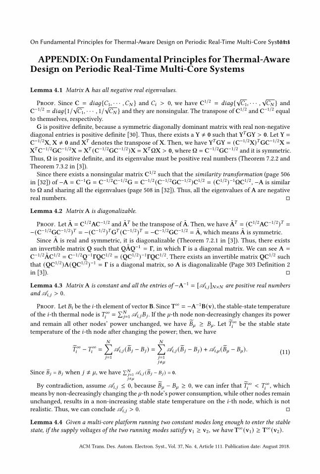
On Fundamental Principles for Thermal-Aware Design on Periodic Real-Time Multi-Core Systems111:1
APPENDIX:OnFundamental Principles for Thermal-AwareDesign on Periodic Real-Time Multi-Core Systems
Lemma 4.1 Matrix A has all negative real eigenvalues.
Proof. Since C = 𝑑𝑖𝑎𝑔𝐶1, · · · ,𝐶𝑁 and 𝐶𝑖 > 0, we have C1/2 = 𝑑𝑖𝑎𝑔√𝐶1, · · · ,
√𝐶𝑁 and
C−1/2 = 𝑑𝑖𝑎𝑔1/√𝐶1, · · · , 1/
√𝐶𝑁 and they are nonsingular. The transpose of C1/2
and C−1/2equal
to themselves, respectively.
G is positive definite, because a symmetric diagonally dominant matrix with real non-negative
diagonal entries is positive definite [30]. Thus, there exists a Y ≠ 0 such that Y𝑇 GY > 0. Let Y =
C−1/2X, X ≠ 0 and X𝑇denotes the transpose of X. Then, we have Y𝑇 GY = (C−1/2X)𝑇 GC−1/2X =
X𝑇 C−1/2GC−1/2X = X𝑇 (C−1/2GC−1/2)X = X𝑇 ΩX > 0, where Ω = C−1/2GC−1/2and it is symmetric.
Thus, Ω is positive definite, and its eigenvalue must be positive real numbers (Theorem 7.2.2 and
Theorem 7.3.2 in [3]).
Since there exists a nonsingular matrix C1/2such that the similarity transformation (page 506
in [32]) of −A = C−1G = C−1/2C−1/2G = C−1/2 (C−1/2GC−1/2)C1/2 = (C1/2)−1ΩC1/2, −A is similar
to Ω and sharing all the eigenvalues (page 508 in [32]). Thus, all the eigenvalues of A are negative
real numbers.
Lemma 4.2 Matrix A is diagonalizable.
Proof. Let A = C1/2AC−1/2and A𝑇
be the transpose of A. Then, we have A𝑇 = (C1/2AC−1/2)𝑇 =
−(C−1/2GC−1/2)𝑇 = −(C−1/2)𝑇 G𝑇 (C−1/2)𝑇 = −C−1/2GC−1/2 = A, which means A is symmetric.
Since A is real and symmetric, it is diagonalizable (Theorem 7.2.1 in [3]). Thus, there exists
an invertible matrix Q such that QAQ−1 = Γ, in which Γ is a diagonal matrix. We can see A =
C−1/2AC1/2 = C−1/2Q−1ΓQC1/2 = (QC1/2)−1ΓQC1/2. There exists an invertible matrix QC1/2
such
that (QC1/2)A(QC1/2)−1 = Γ is a diagonal matrix, so A is diagonalizable (Page 303 Definition 2
in [3]).
Lemma 4.3 Matrix A is constant and all the entries of −A−1 = [A𝑖, 𝑗 ]𝑁×𝑁 are positive real numbersand A𝑖, 𝑗 > 0.
Proof. Let 𝐵𝑖 be the 𝑖-th element of vector B. Since T∞ = −A−1B(v), the stable-state temperature
of the 𝑖-th thermal node is 𝑇∞𝑖 =
∑𝑁𝑗=1 A𝑖, 𝑗𝐵 𝑗 . If the `-th node non-decreasingly changes its power
and remain all other nodes’ power unchanged, we have 𝐵` ≥ 𝐵` . Let 𝑇∞𝑖 be the stable state
temperature of the 𝑖-th node after changing the power; then, we have
𝑇∞𝑖 −𝑇∞
𝑖 =
𝑁∑𝑗=1
A𝑖, 𝑗 (𝐵 𝑗 − 𝐵 𝑗 ) =𝑁∑𝑗=1𝑗≠`
A𝑖, 𝑗 (𝐵 𝑗 − 𝐵 𝑗 ) + A𝑖,` (𝐵` − 𝐵`).(11)
Since 𝐵 𝑗 = 𝐵 𝑗 when 𝑗 ≠ `, we have∑𝑁
𝑗=1𝑗≠`
A𝑖,𝑗 (𝐵 𝑗 − 𝐵 𝑗 ) = 0.
By contradiction, assume A𝑖, 𝑗 ≤ 0, because 𝐵` − 𝐵` ≥ 0, we can infer that 𝑇∞𝑖 < 𝑇∞
𝑖 , which
means by non-decreasingly changing the `-th node’s power consumption, while other nodes remain
unchanged, results in a non-increasing stable state temperature on the 𝑖-th node, which is not
realistic. Thus, we can conclude A𝑖, 𝑗 > 0.
Lemma 4.4 Given a multi-core platform running two constant modes long enough to enter the stablestate, if the supply voltages of the two running modes satisfy v1 ≥ v2, we have T∞ (v1) ≥ T∞ (v2).
ACM Trans. Des. Autom. Electron. Syst., Vol. 37, No. 4, Article 111. Publication date: August 2018.

111:2 Sha and Bankar, et al.
Proof. From (1), we have T∞ (v1) − T∞ (v2) = −A−1 [B(v1) − B(v2)]. Since B(v1) − B(v2) ≥ 0when v1 ≥ v2, and −A−1
contains all positive entries (Lemma 4.3), we have T∞ (v1) ≥ T∞ (v2).
Lemma 4.5 All the elements in matrix (I − K)−1 are positive and each entry monotonically decreaseswith 𝑙 , where K = 𝑒A𝑙 , 𝑙 > 0.
Proof. [Part 1]: Prove (I − K)−1 > 0.Let 𝜌 (𝑒A𝑙 ) denote the spectral radius of 𝑒A𝑙
, we have 𝜌 (𝑒A𝑙 ) = 𝑚𝑎𝑥 |𝑒_𝑖𝑙 | (page 497 in [32]).
Because for all _𝑖 > 0, we have for all 0 < 𝑒−_𝑖𝑙 < 1 and |𝑒_𝑖𝑙 | < 1, so 𝜌 (𝑒A𝑙 ) < 1. Since 𝜌 (𝑒A𝑙 ) < 1,
we have lim𝐻→∞ (𝑒A𝑙 )𝐻 = 0.We adopt the Neumann Series (page 618 in [32]) by geometric series formula for matrices
version, which can be proved similarly as the geometric series formula for numbers, i.e.
∑𝐻ℎ=0
Kℎ =
(I − K𝐻+1) (I − K)−1. Thus, we have (I − K)−1 = ∑∞ℎ=0
Kℎ.
Since all the elements of 𝑒A𝑙are positive (Lemma 1 in [18]), we can conclude (I − 𝑒A𝑙 )−1 only
contains positive elements.
[Part 2]: Prove each element in (I − K)−1 monotonically decreases with 𝑙 .
Let K𝑘,𝑗 , `𝑘,𝑗 and 𝜙𝑘,𝑗 be the element on the 𝑘-th row and 𝑗-th column of (I − K)−1, W and W−1,
respectively, 𝑘, 𝑗 ∈ 1, · · · , 𝑁 . Diagonalize (I − K)−1 by (5), we have
(I − 𝑒A𝑙 )−1 = (I − W · 𝑒D𝑙 · W−1)−1
=(W · W−1 − W · 𝑒D𝑙 · W−1)−1
=(W · (I − 𝑒D𝑙 ) · W−1)−1 = W · 𝑒 (I−D𝑙)−1 · W−1
=W · 𝑑𝑖𝑎𝑔(1 − 𝑒−_1𝑙 )−1, · · · , (1 − 𝑒−_𝑁 𝑙 )−1 · W−1.
(12)
Thus, we have K𝑘,𝑗 =∑𝑁
𝑖=1 `𝑘,𝑖 · 𝜙𝑖, 𝑗 · (1 − 𝑒−_𝑖𝑙 )−1. To prove K𝑘,𝑗 monotonically decreases with 𝑙
while `𝑘,𝑗 and 𝜙𝑘,𝑗 are constants, since K𝑘,𝑗 > 0, we need to prove each eigenvalue (1 − 𝑒−_𝑖𝑙 )−1monotonically decreases with 𝑙 .
Since −_𝑖 < 0 and 𝑙 > 0, 𝑒−_𝑖𝑙 monotonically decreases with 𝑙 and 0 < 𝑒−_𝑖𝑙 < 1. Then, (1− 𝑒−_𝑖𝑙 )monotonically increases with 𝑙 and 0 < 1 − 𝑒−_𝑖𝑙 < 1. Thus, (1 − 𝑒−_𝑖𝑙 )−1 > 0 and it monotonically
decreases with 𝑙 .
Theorem 4.6 Let 𝑙 > 0 and 0 ≤ T ≤ (T∞ (vmax) − T∞ (vmin)), then (I − K)T ≥ 0, where K = 𝑒A𝑙 ,vmax = [𝑣𝑚𝑎𝑥,𝑖 ]𝑁×1 and vmin = [𝑣𝑚𝑖𝑛,𝑖 ]𝑁×1. 𝑣𝑚𝑎𝑥,𝑖 and 𝑣𝑚𝑖𝑛,𝑖 denote the maximum and minimumavailable supply voltage on the 𝑖-th node, respectively.
Proof. Consider a state interval I𝑞 = [𝑡𝑞−1, 𝑡𝑞] starts at T0 = T∞ (vmax) and runs at the mode
with supply voltage v. Since v ≤ vmax, we have T∞ (vmax) − T∞ (v) ≥ 0 (Lemma 4.4). Because
given a multi-core platform and a state interval, the temperature on each core must monotonically
decrease if all the cores’ starting temperature is higher than the running mode’s stable state
temperature (Theorem 5 in [18]), we have ∀𝑡 ∈ [𝑡𝑞−1, 𝑡𝑞], T(𝑡) ≤ T∞ (vmax). Thus, from (3), T(𝑡)can be expressed as
𝑒A(𝑡−𝑡𝑞−1)T∞ (vmax) + (I − 𝑒A(𝑡−𝑡𝑞−1) )T∞ (v) ≤ T∞ (vmax)⇒ (I − 𝑒A(𝑡−𝑡𝑞−1) ) (T∞ (vmax) − T∞ (v)) ≥ 0
(13)
In contrary, if T0 = T∞ (vmin), and the system executes at v with v ≥ vmin, the temperature must
monotonically increase (Theorem 5 in [18]). Thus, we have
𝑒A(𝑡−𝑡𝑞−1)T∞ (vmin) + (I − 𝑒A(𝑡−𝑡𝑞−1) )T∞ (v) ≥ T∞ (vmin)⇒ (I − 𝑒A(𝑡−𝑡𝑞−1) ) (T∞ (v) − T∞ (vmin)) ≥ 0
(14)
ACM Trans. Des. Autom. Electron. Syst., Vol. 37, No. 4, Article 111. Publication date: August 2018.
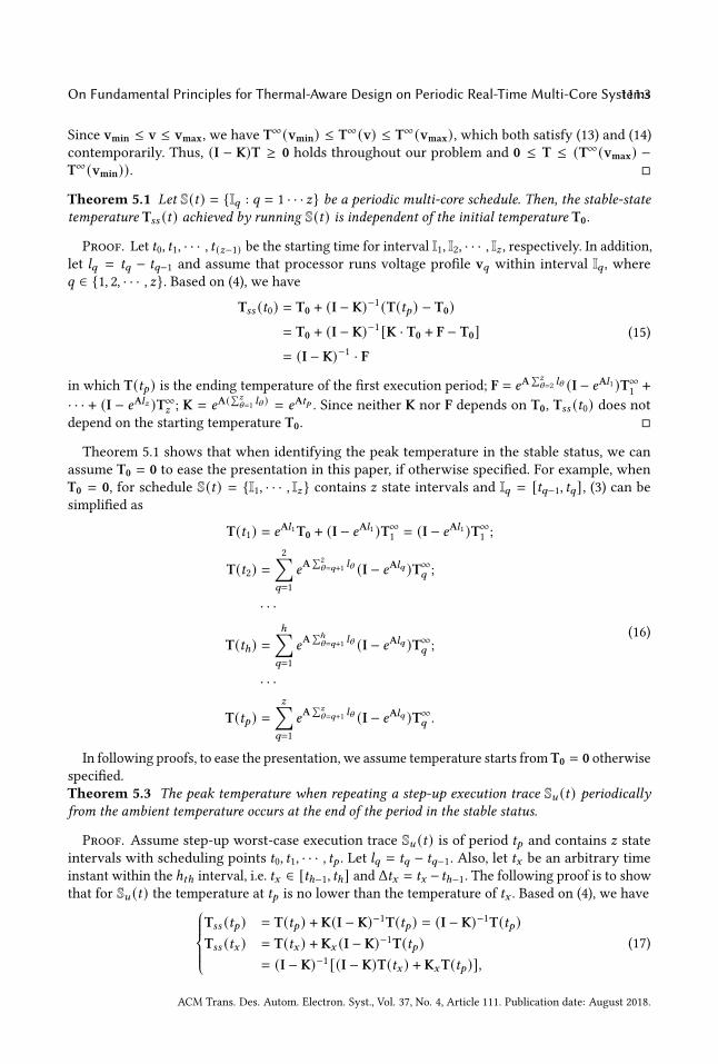
On Fundamental Principles for Thermal-Aware Design on Periodic Real-Time Multi-Core Systems111:3
Since vmin ≤ v ≤ vmax, we have T∞ (vmin) ≤ T∞ (v) ≤ T∞ (vmax), which both satisfy (13) and (14)
contemporarily. Thus, (I − K)T ≥ 0 holds throughout our problem and 0 ≤ T ≤ (T∞ (vmax) −T∞ (vmin)).
Theorem 5.1 Let S(𝑡) = I𝑞 : 𝑞 = 1 · · · 𝑧 be a periodic multi-core schedule. Then, the stable-statetemperature T𝑠𝑠 (𝑡) achieved by running S(𝑡) is independent of the initial temperature T0.
Proof. Let 𝑡0, 𝑡1, · · · , 𝑡 (𝑧−1) be the starting time for interval I1, I2, · · · , I𝑧 , respectively. In addition,
let 𝑙𝑞 = 𝑡𝑞 − 𝑡𝑞−1 and assume that processor runs voltage profile v𝑞 within interval I𝑞 , where𝑞 ∈ 1, 2, · · · , 𝑧. Based on (4), we have
T𝑠𝑠 (𝑡0) = T0 + (I − K)−1 (T(𝑡𝑝 ) − T0)= T0 + (I − K)−1 [K · T0 + F − T0]= (I − K)−1 · F
(15)
in which T(𝑡𝑝 ) is the ending temperature of the first execution period; F = 𝑒A∑𝑧
\=2𝑙\ (I − 𝑒A𝑙1 )T∞
1+
· · · + (I − 𝑒A𝑙𝑧 )T∞𝑧 ; K = 𝑒A(∑𝑧
\=1𝑙\ ) = 𝑒A𝑡𝑝
. Since neither K nor F depends on T0, T𝑠𝑠 (𝑡0) does notdepend on the starting temperature T0.
Theorem 5.1 shows that when identifying the peak temperature in the stable status, we can
assume T0 = 0 to ease the presentation in this paper, if otherwise specified. For example, when
T0 = 0, for schedule S(𝑡) = I1, · · · , I𝑧 contains 𝑧 state intervals and I𝑞 = [𝑡𝑞−1, 𝑡𝑞], (3) can be
simplified as
T(𝑡1) = 𝑒A𝑙1T0 + (I − 𝑒A𝑙1 )T∞1= (I − 𝑒A𝑙1 )T∞
1;
T(𝑡2) =2∑
𝑞=1
𝑒A∑
2
\=𝑞+1 𝑙\ (I − 𝑒A𝑙𝑞 )T∞𝑞 ;
· · ·
T(𝑡ℎ) =ℎ∑
𝑞=1
𝑒A∑ℎ
\=𝑞+1 𝑙\ (I − 𝑒A𝑙𝑞 )T∞𝑞 ;
· · ·
T(𝑡𝑝 ) =𝑧∑
𝑞=1
𝑒A∑𝑧
\=𝑞+1 𝑙\ (I − 𝑒A𝑙𝑞 )T∞𝑞 .
(16)
In following proofs, to ease the presentation, we assume temperature starts from T0 = 0 otherwise
specified.
Theorem 5.3 The peak temperature when repeating a step-up execution trace S𝑢 (𝑡) periodicallyfrom the ambient temperature occurs at the end of the period in the stable status.
Proof. Assume step-up worst-case execution trace S𝑢 (𝑡) is of period 𝑡𝑝 and contains 𝑧 state
intervals with scheduling points 𝑡0, 𝑡1, · · · , 𝑡𝑝 . Let 𝑙𝑞 = 𝑡𝑞 − 𝑡𝑞−1. Also, let 𝑡𝑥 be an arbitrary time
instant within the ℎ𝑡ℎ interval, i.e. 𝑡𝑥 ∈ [𝑡ℎ−1, 𝑡ℎ] and Δ𝑡𝑥 = 𝑡𝑥 − 𝑡ℎ−1. The following proof is to showthat for S𝑢 (𝑡) the temperature at 𝑡𝑝 is no lower than the temperature of 𝑡𝑥 . Based on (4), we have
T𝑠𝑠 (𝑡𝑝 ) = T(𝑡𝑝 ) + K(I − K)−1T(𝑡𝑝 ) = (I − K)−1T(𝑡𝑝 )T𝑠𝑠 (𝑡𝑥 ) = T(𝑡𝑥 ) + K𝑥 (I − K)−1T(𝑡𝑝 )
= (I − K)−1 [(I − K)T(𝑡𝑥 ) + K𝑥T(𝑡𝑝 )],(17)
ACM Trans. Des. Autom. Electron. Syst., Vol. 37, No. 4, Article 111. Publication date: August 2018.

111:4 Sha and Bankar, et al.
core_N
core_N
v1 v2 vh… …
v2…
core_N
……
vzcore_1
core_1
v1 v2 …
0 tpth… …tx
…core_1
t(h-1)
vh
Time
Speed
v1 vh
Fig. 11. Proof illustration for Theorem 5.3
in whichK = 𝑒A𝑡𝑝andK𝑥 = 𝑒A(Δ𝑡𝑥+
∑𝑞−1\=1
𝑙\ ). Since (I−K)−1 contains all positive elements (Lemma 4.5),
to prove T𝑠𝑠 (𝑡𝑝 ) ≥ T𝑠𝑠 (𝑡𝑥 ), we want to prove T(𝑡𝑝 ) − [(I − K)T(𝑡𝑥 ) + K𝑥T(𝑡𝑝 )] ≥ 0, which is
equivalent to prove
T(𝑡𝑝 ) − [(I − K)T(𝑡𝑥 ) + K𝑥T(𝑡𝑝 )] = (I − K𝑥 ) (I − K) [(I − K)−1T(𝑡𝑝 ) − (I − K𝑥 )−1T(𝑡𝑥 )] ≥ 0. (18)
Since (I − K𝑥 ) (I − K)T ≥ 0, if T ≥ 0 (Theorem 4.6), we need to prove that (I − K)−1T(𝑡𝑝 ) − (I −K𝑥 )−1T(𝑡𝑥 ) ≥ 0. From (4), (I − K)−1T(𝑡𝑝 ) is the stable status temperature at time 𝑡𝑝 of schedule
S𝑢 (𝑡), and (I − K𝑥 )−1T(𝑡𝑥 ) is the stable status temperature at time 𝑡𝑥 for the S′𝑢 (𝑡) that consists ofall state intervals of S𝑢 (𝑡) within interval [0, 𝑡𝑥 ].To prove S𝑢 (𝑡) has a higher peak temperature than S′𝑢 (𝑡), we define an intermediate schedule
S𝑢 (𝑡) with period 𝑡𝑝 , which consists of all the state intervals of S′𝑢 (𝑡) within interval [0, 𝑡ℎ−1],and keeps constant voltage vℎ within [𝑡ℎ−1, 𝑡𝑝 ], as shown in Figure 11. Then we need to prove
T𝑠𝑠 (S𝑢 (𝑡𝑝 )) ≥ T𝑠𝑠 (S𝑢 (𝑡𝑝 )) ≥ T𝑠𝑠 (S′𝑢 (𝑡𝑥 )).First, we prove T𝑠𝑠 (S𝑢 (𝑡𝑝 )) ≥ T𝑠𝑠 (S𝑢 (𝑡𝑝 )), in which T𝑠𝑠 (S𝑢 (𝑡𝑝 )) = (I − K)−1T(S𝑢 (𝑡𝑝 )) and
T𝑠𝑠 (S𝑢 (𝑡𝑝 )) = (I−K)−1T(S𝑢 (𝑡𝑝 )) from (4). K is identical for both schedule S𝑢 (𝑡) and S𝑢 (𝑡) becausetheir periods are the same. Then, we need to prove T(S𝑢 (𝑡𝑝 )) ≥ T(S𝑢 (𝑡𝑝 )), which are the ending
temperatures of the first period.
Let v𝑞 and v𝑞 be the supply voltage of the 𝑞-th interval of schedule S𝑢 (𝑡) and S𝑢 (𝑡), respectively.Let T∞
𝑞 = T∞ (v𝑞) and T∞𝑞 = T∞ (v𝑞). We know v𝑞 = v𝑞 and T∞
𝑞 = T∞𝑞 when 𝑞 ∈ 1, · · · , ℎ; v𝑞 ≥ v𝑞
and T∞𝑞 ≥ T∞
𝑞 when 𝑞 ∈ ℎ + 1, · · · , 𝑧, since S𝑢 (𝑡) is in a step-up pattern (Definition 5.2). Then,
from (16), we have
T(S𝑢 (𝑡𝑝 )) − T(S𝑢 (𝑡𝑝 ))
=
ℎ∑𝑞=1
(𝑒
A∑𝑧
\=𝑞+1 𝑙\ (I − 𝑒A𝑙𝑞 ) (T∞𝑞 − T∞
𝑞 ))+
𝑧∑𝑞=ℎ+1
(𝑒
A∑𝑧
\=𝑞+1 𝑙\ (I − 𝑒A𝑙𝑞 ) (T∞𝑞 − T∞
𝑞 ))
=0 +𝑧∑
𝑞=ℎ+1
(𝑒
A∑𝑧
\=𝑞+1 𝑙\ (I − 𝑒A𝑙𝑞 ) (T∞𝑞 − T∞
𝑞 )).
(19)
Since 𝑒A∑𝑧
\=𝑞+1 𝑙\contains all positive elements (Lemma 1 in [18]), we need to prove (I−𝑒A𝑙𝑞 ) (T∞
𝑞 −T∞𝑞 ) ≥ 0 when 𝑞 ∈ ℎ + 1, · · · , 𝑧. Since T∞
𝑞 ≥ T∞𝑞 when 𝑞 ∈ ℎ + 1, · · · , 𝑧, the conclusion is
proved (Theorem 4.6).
Next, we prove T𝑠𝑠 (S𝑢 (𝑡𝑝 )) ≥ T𝑠𝑠 (S′𝑢 (𝑡𝑥 )). Starting from the same temperature, if we can prove
that for each consecutive period the ending temperature of S𝑢 (𝑡) is greater than that of S′𝑢 (𝑡),
ACM Trans. Des. Autom. Electron. Syst., Vol. 37, No. 4, Article 111. Publication date: August 2018.
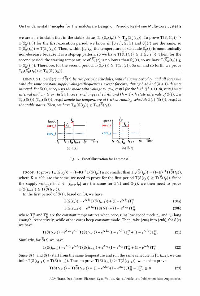
On Fundamental Principles for Thermal-Aware Design on Periodic Real-Time Multi-Core Systems111:5
we are able to claim that in the stable status T𝑠𝑠 (S𝑢 (𝑡𝑝 )) ≥ T𝑠𝑠 (S′𝑢 (𝑡𝑥 )). To prove T(S𝑢 (𝑡𝑝 )) ≥T(S′𝑢 (𝑡𝑥 )) for the first execution period, we know in [0, 𝑡𝑥 ], S𝑢 (𝑡) and S′𝑢 (𝑡) are the same, so
T(S𝑢 (𝑡𝑥 )) = T(S′𝑢 (𝑡𝑥 )). Then, within [𝑡𝑥 , 𝑡𝑝 ] the temperature of schedule S𝑢 (𝑡) is monotonically
non-decrease because it is a step-up pattern, so we have T(S𝑢 (𝑡𝑝 )) ≥ T(S𝑢 (𝑡𝑥 )). Then, for thesecond period, the starting temperature of S𝑢 (𝑡) is no lower than S′𝑢 (𝑡), so we have T(S𝑢 (𝑡𝑥 )) ≥T(S′𝑢 (𝑡𝑥 )). Therefore, for the second period, T(S𝑢 (𝑡)) ≥ T(S𝑢 (𝑡)). So on and so forth, we prove
T𝑠𝑠 (S𝑢 (𝑡𝑝 )) ≥ T𝑠𝑠 (S′𝑢 (𝑡𝑥 )).
Lemma 8.1. Let S(𝑡) and S(𝑡) be two periodic schedules, with the same period 𝑡𝑝 , and all cores runwith the same constant supply voltages/frequencies, except for 𝑐𝑜𝑟𝑒𝑖 during ℎ-th and (ℎ + 1)-th stateinterval. For S(𝑡), 𝑐𝑜𝑟𝑒𝑖 uses the mode with voltage 𝑣𝐿 (𝑣𝐻 , resp.) for the ℎ-th ((ℎ + 1)-th, resp.) stateinterval and 𝑣𝐻 ≥ 𝑣𝐿 . In S(𝑡), 𝑐𝑜𝑟𝑒𝑖 exchanges the ℎ-th and (ℎ + 1)-th state intervals of S(𝑡). LetT𝑠𝑠 (S(𝑡)) (T𝑠𝑠 (S(𝑡)), resp.) denote the temperature at 𝑡 when running schedule S(𝑡) (S(𝑡)), resp.) inthe stable status. Then, we have T𝑠𝑠 (S(𝑡𝑝 )) ≥ T𝑠𝑠 (S(𝑡𝑝 )).
core_iSpeed
core_j
t0 Timetpth-1 th th+1
lHlL
(a) S(𝑡 )
core_iSpeed
core_j
t0 Timetp~th-1th th+1
lHlL
(b) S(𝑡 )
Fig. 12. Proof illustration for Lemma 8.1
Proof. To proveT𝑠𝑠 (S(𝑡𝑝 )) = (I−K)−1T(S(𝑡𝑝 )) is no smaller thanT𝑠𝑠 (S(𝑡𝑝 )) = (I−K)−1T(S(𝑡𝑝 )),where K = 𝑒A𝑡𝑝
are the same, we need to prove for the first period T(S(𝑡𝑝 )) ≥ T(S(𝑡𝑝 )). Sincethe supply voltage in 𝑡 ∈ [𝑡ℎ+1, 𝑡𝑝 ] are the same for S(𝑡) and S(𝑡), we then need to prove
T(S(𝑡ℎ+1)) ≥ T(S(𝑡ℎ+1)).In the first period of S(𝑡), based on (3), we have
T(S(𝑡ℎ)) = 𝑒A·𝑙𝐿T(S(𝑡ℎ−1)) + (I − 𝑒A·𝑙𝐿 )T∞𝐿 (20a)
T(S(𝑡ℎ+1)) = 𝑒A·𝑙𝐻 T(S(𝑡ℎ)) + (I − 𝑒A·𝑙𝐻 )T∞𝐻 , (20b)
where T∞𝐿and T∞
𝐻are the constant temperatures when 𝑐𝑜𝑟𝑒𝑖 runs low-speed mode 𝑣𝐿 and 𝑣𝐻 long
enough, respectively, while other cores keep constant mode. Then, take (20a) into (20b), for S(𝑡)we have
T(S(𝑡ℎ+1)) =𝑒A·𝑙𝐻 𝑒A·𝑙𝐿T(S(𝑡ℎ−1)) + 𝑒A·𝑙𝐻 (I − 𝑒A𝑙𝐿 )T∞𝐿 + (I − 𝑒A·𝑙𝐻 )T∞
𝐻 . (21)
Similarly, for S(𝑡) we have
T(S(𝑡ℎ+1)) =𝑒A·𝑙𝐻 𝑒A·𝑙𝐿T(S(𝑡ℎ−1)) + 𝑒A·𝑙𝐿 (I − 𝑒A𝑙𝐻 )T∞𝐻 + (I − 𝑒A·𝑙𝐿 )T∞
𝐿 . (22)
Since S(𝑡) and S(𝑡) start from the same temperature and run the same schedule in [0, 𝑡ℎ−1], we caninfer T(S(𝑡ℎ−1)) = T(S(𝑡ℎ−1)). Thus, to prove T(S(𝑡ℎ+1)) ≥ T(S(𝑡ℎ+1)), we need to prove
T(S(𝑡ℎ+1)) − T(S(𝑡ℎ+1)) = (I − 𝑒A𝑙𝐻 ) (I − 𝑒A𝑙𝐿 ) (T∞𝐻 − T∞
𝐿 ) ≥ 0 (23)
ACM Trans. Des. Autom. Electron. Syst., Vol. 37, No. 4, Article 111. Publication date: August 2018.
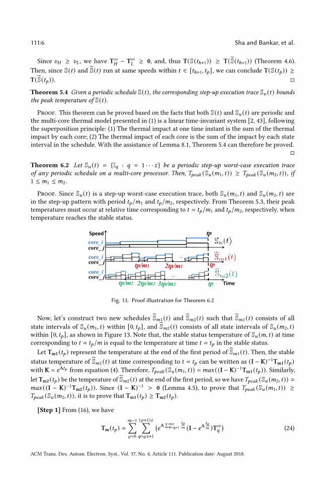
111:6 Sha and Bankar, et al.
Since 𝑣𝐻 ≥ 𝑣𝐿 , we have T∞𝐻
− T∞𝐿
≥ 0, and, thus T(S(𝑡ℎ+1)) ≥ T(S(𝑡ℎ+1)) (Theorem 4.6).
Then, since S(𝑡) and S(𝑡) run at same speeds within 𝑡 ∈ [𝑡ℎ+1, 𝑡𝑝 ], we can conclude T(S(𝑡𝑝 )) ≥T(S(𝑡𝑝 )).
Theorem 5.4 Given a periodic schedule S(𝑡), the corresponding step-up execution trace S𝑢 (𝑡) boundsthe peak temperature of S(𝑡).
Proof. This theorem can be proved based on the facts that both S(𝑡) and S𝑢 (𝑡) are periodic andthe multi-core thermal model presented in (1) is a linear time-invariant system [2, 43], following
the superposition principle: (1) The thermal impact at one time instant is the sum of the thermal
impact by each core; (2) The thermal impact of each core is the sum of the impact by each state
interval in the schedule. With the assistance of Lemma 8.1, Theorem 5.4 can therefore be proved.
Theorem 6.2 Let S𝑢 (𝑡) = I𝑞 : 𝑞 = 1 · · · 𝑧 be a periodic step-up worst-case execution traceof any periodic schedule on a multi-core processor. Then, 𝑇𝑝𝑒𝑎𝑘 (S𝑢 (𝑚1, 𝑡)) ≥ 𝑇𝑝𝑒𝑎𝑘 (S𝑢 (𝑚2, 𝑡)), if1 ≤ 𝑚1 ≤ 𝑚2.
Proof. Since S𝑢 (𝑡) is a step-up worst-case execution trace, both S𝑢 (𝑚1, 𝑡) and S𝑢 (𝑚2, 𝑡) arein the step-up pattern with period 𝑡𝑝/𝑚1 and 𝑡𝑝/𝑚2, respectively. From Theorem 5.3, their peak
temperatures must occur at relative time corresponding to 𝑡 = 𝑡𝑝/𝑚1 and 𝑡𝑝/𝑚2, respectively, when
temperature reaches the stable status.
tptp/m1core_ j 2tp/m1
Time
…
…core_ jcore_i
tp
core_icore_ jcore_iSpeed
tp/m2 2tp/m2 3tp/m2 tp
Fig. 13. Proof illustration for Theorem 6.2
Now, let’s construct two new schedules S𝑚1 (𝑡) and S𝑚2 (𝑡) such that S𝑚1 (𝑡) consists of allstate intervals of S𝑢 (𝑚1, 𝑡) within [0, 𝑡𝑝 ], and S𝑚2 (𝑡) consists of all state intervals of S𝑢 (𝑚2, 𝑡)within [0, 𝑡𝑝 ], as shown in Figure 13. Note that, the stable status temperature of S𝑢 (𝑚, 𝑡) at time
corresponding to 𝑡 = 𝑡𝑝/𝑚 is equal to the temperature at time 𝑡 = 𝑡𝑝 in the stable status.
Let Tm1 (𝑡𝑝 ) represent the temperature at the end of the first period of S𝑚1 (𝑡). Then, the stablestatus temperature of S𝑚1 (𝑡) at time corresponding to 𝑡 = 𝑡𝑝 can be written as (I − K)−1Tm1 (𝑡𝑝 )with K = 𝑒A𝑡𝑝
from equation (4). Therefore, 𝑇𝑝𝑒𝑎𝑘 (S𝑢 (𝑚1, 𝑡)) =𝑚𝑎𝑥 ((I − K)−1Tm1 (𝑡𝑝 )). Similarly,
let Tm2 (𝑡𝑝 ) be the temperature of S𝑚2 (𝑡) at the end of the first period, so we have𝑇𝑝𝑒𝑎𝑘 (S𝑢 (𝑚2, 𝑡)) =𝑚𝑎𝑥 ((I − K)−1Tm2 (𝑡𝑝 )). Since (I − K)−1 > 0 (Lemma 4.5), to prove that 𝑇𝑝𝑒𝑎𝑘 (S𝑢 (𝑚1, 𝑡)) ≥𝑇𝑝𝑒𝑎𝑘 (S𝑢 (𝑚2, 𝑡)), it is to prove that Tm1 (𝑡𝑝 ) ≥ Tm2 (𝑡𝑝 ).
[Step 1] From (16), we have
Tm (𝑡𝑝 ) =𝑚−1∑𝜚=0
(𝜚+1)𝑧∑𝑞=𝜚𝑧+1
(𝑒
A∑𝑚𝑧
\=𝑞+1𝑙\𝑚 (I − 𝑒A
𝑙𝑞
𝑚 )T∞𝑞
)(24)
ACM Trans. Des. Autom. Electron. Syst., Vol. 37, No. 4, Article 111. Publication date: August 2018.

On Fundamental Principles for Thermal-Aware Design on Periodic Real-Time Multi-Core Systems111:7
in which𝑚 =𝑚1 for S𝑚1 (𝑡) or𝑚 =𝑚2 for S𝑚2 (𝑡) schedule.Let Tm1 (𝑡𝑝 ) and Tm2 (𝑡𝑝 ) denote the 𝑞-th element when𝑚 =𝑚1 and𝑚 =𝑚2 in (24), respectively.
To prove Tm1 (𝑡𝑝 ) − Tm2 (𝑡𝑝 ) ≥ 0, we need to prove fro each 𝑞, there exsists Tm1 (𝑡𝑝 ) ≥ Tm2 (𝑡𝑝 ),where
Tm (𝑡𝑝 ) =𝑚−1∑𝜚=0
𝑒A∑𝑚𝑧
\=𝜚𝑧+𝑞+1𝑙\𝑚 (I − 𝑒A
𝑙𝜚𝑧+𝑞𝑚 )T∞
𝜚𝑧+𝑞 (25)
Since S𝑢 (𝑚1, 𝑡) and S𝑢 (𝑚2, 𝑡) are both periodical, for all positive integer 𝜚 , we have 𝑙𝜚𝑧+𝑞 = 𝑙𝑞 and
T∞𝜚𝑧+𝑞 = T∞
𝑞 . Then, (25) indeed is the sum of a geometric matrices series [32], which are constituted
by the first term as 𝑒A∑𝑚𝑧
\=(𝑚−1)𝑧+𝑞+1𝑙\𝑚 (I−𝑒A
𝑙𝑞
𝑚 )T∞𝑞 , equal ratio as 𝑒A𝑡𝑝/𝑚
, and totally contains𝑚 terms.
Using the sum of geometric matrices series [32], we have
Tm (𝑡𝑝 ) = 𝑒A∑𝑚𝑧
\=(𝑚−1)𝑧+𝑞+1𝑙\𝑚 (I − 𝑒A
𝑚𝑡𝑝
𝑚 ) (I − 𝑒A𝑡𝑝
𝑚 )−1 (I − 𝑒A𝑙𝑞
𝑚 )T∞𝑞
=𝑒A∑𝑧
\=𝑞+1𝑙\𝑚 (I − 𝑒A𝑡𝑝 ) (I − 𝑒A
𝑡𝑝
𝑚 )−1 (I − 𝑒A· 𝑙𝑞𝑚 )T∞
𝑞
=Θ(𝑚) (I − 𝑒A𝑡𝑝 )T∞𝑞
(26)
where
Θ(𝑚) = 𝑒A 𝜛𝑚 (I − 𝑒A
𝑡𝑝
𝑚 )−1 (I − 𝑒A𝑙𝑞
𝑚 ). (27)
and 𝜛 =∑𝑧
\=𝑞+1 𝑙\ .
[Step 2] To compare Tm1 (𝑡𝑝 ) and Tm2 (𝑡𝑝 ) from (26) by different𝑚, essentially, it can be suffi-
ciently proved by showing that each eigenvalue of (27) monotonically decreases with𝑚. From (5),
we can diagonalize Θ(𝑚) as
Θ(𝑚) = W𝑑𝑖𝑎𝑔Υ1 (𝑚), · · · , Υ𝑁 (𝑚)W−1. (28)
where
Υ𝑖 (𝑚) = 𝑒−_𝑖𝜛𝑚 (1 − 𝑒−_𝑖
𝑙𝑞
𝑚 )1 − 𝑒−_𝑖
𝑡𝑝
𝑚
. (29)
We then prove Υ𝑖 (𝑚) monotonically decreases with 𝑚 as follows. Note that _𝑖 , 𝜛 𝑙𝑞 and 𝑡𝑝 are
constants. Since 𝑒−_𝑖𝜛/𝑚monotonically decreases with𝑚, we then need to prove
1−𝑒−_𝑖𝑙𝑞/𝑚
1−𝑒−_𝑖𝑡𝑝 /𝑚 mono-
tonically decreases with𝑚 too.
Let 𝐹 (𝜑) = 1−𝑒−_𝑖𝑙𝑞/𝑚
1−𝑒−_𝑖𝑡𝑝 /𝑚 = 1−𝑒−𝜎1𝜑1−𝑒−𝜎2𝜑 , where 𝜎1 = _𝑖𝑙𝑞 , 𝜎2 = _𝑖𝑡𝑝 and 𝜑 = 1/𝑚. To prove 𝐹 (𝑚)
monotonically decrease with𝑚, we need to prove 𝐹 (𝜑) = 1−𝑒−𝜑𝜎1
1−𝑒−𝜑𝜎2monotonically increase with 𝜑 ,
where 𝜑 > 0 and 𝜎2 > 𝜎1 > 0, which is equivalent to prove
𝐹 ′(𝜑) = (𝜎2 − 𝜎1)𝑒−(𝜎1+𝜎2)𝜑 + 𝜎1𝑒−𝜎1𝜑 − 𝜎2𝑒−𝜎2𝜑(1 − 𝑒−𝜎2𝜑 )2 > 0. (30)
Let
𝐹 ′(𝜑)𝐹 (𝜑) =
𝜎1𝑒−𝜎1𝜑
1 − 𝑒−𝜎1𝜑 − 𝜎2𝑒−𝜎2𝜑
1 − 𝑒−𝜎2𝜑 = b (𝜎1) − b (𝜎2) (31)
in which b (𝜎) = 𝜎𝑒−𝜎𝜑
1−𝑒−𝜎𝜑 . Since 𝐹 (𝜑) > 0, we need to prove b (𝜎) monotonically decreases with 𝜎 ,
i.e. b ′(𝜎) =𝑒−𝜎𝜑 (1−𝜎𝜑−𝑒−𝜎𝜑 )
(1−𝑒−𝜎𝜑 )2 < 0. Let 𝐻 (𝜑) = 1 − 𝜎𝜑 − 𝑒−𝜎𝜑 , we can see 𝐻 (0) = 0 and 𝐻 ′(𝜑) =
𝜎 (−1 + 𝑒−𝜎𝜑 ) < 0 when 𝜑 > 0. Thus, we can infer b ′(𝜎) < 0.
ACM Trans. Des. Autom. Electron. Syst., Vol. 37, No. 4, Article 111. Publication date: August 2018.
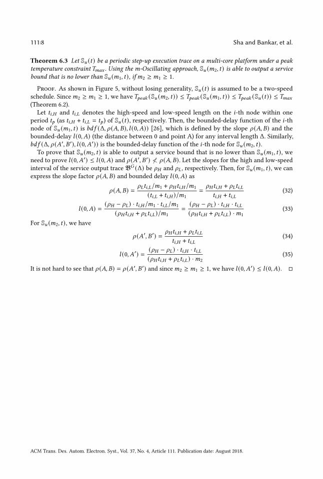
111:8 Sha and Bankar, et al.
Theorem 6.3 Let S𝑢 (𝑡) be a periodic step-up execution trace on a multi-core platform under a peaktemperature constraint 𝑇𝑚𝑎𝑥 . Using the m-Oscillating approach, S𝑢 (𝑚2, 𝑡) is able to output a servicebound that is no lower than S𝑢 (𝑚1, 𝑡), if𝑚2 ≥ 𝑚1 ≥ 1.
Proof. As shown in Figure 5, without losing generality, S𝑢 (𝑡) is assumed to be a two-speed
schedule. Since𝑚2 ≥ 𝑚1 ≥ 1, we have 𝑇𝑝𝑒𝑎𝑘 (S𝑢 (𝑚2, 𝑡)) ≤ 𝑇𝑝𝑒𝑎𝑘 (S𝑢 (𝑚1, 𝑡)) ≤ 𝑇𝑝𝑒𝑎𝑘 (S𝑢 (𝑡)) ≤ 𝑇𝑚𝑎𝑥
(Theorem 6.2).
Let 𝑡𝑖,𝐻 and 𝑡𝑖,𝐿 denotes the high-speed and low-speed length on the 𝑖-th node within one
period 𝑡𝑝 (as 𝑡𝑖,𝐻 + 𝑡𝑖,𝐿 = 𝑡𝑝 ) of S𝑢 (𝑡), respectively. Then, the bounded-delay function of the 𝑖-th
node of S𝑢 (𝑚1, 𝑡) is 𝑏𝑑 𝑓 (Δ, 𝜌 (𝐴, 𝐵), 𝑙 (0, 𝐴)) [26], which is defined by the slope 𝜌 (𝐴, 𝐵) and the
bounded-delay 𝑙 (0, 𝐴) (the distance between 0 and point A) for any interval length Δ. Similarly,
𝑏𝑑 𝑓 (Δ, 𝜌 (𝐴′, 𝐵′), 𝑙 (0, 𝐴′)) is the bounded-delay function of the 𝑖-th node for S𝑢 (𝑚2, 𝑡).To prove that S𝑢 (𝑚2, 𝑡) is able to output a service bound that is no lower than S𝑢 (𝑚1, 𝑡), we
need to prove 𝑙 (0, 𝐴′) ≤ 𝑙 (0, 𝐴) and 𝜌 (𝐴′, 𝐵′) ≮ 𝜌 (𝐴, 𝐵). Let the slopes for the high and low-speed
interval of the service output trace 𝔅𝐺 (Δ) be 𝜌𝐻 and 𝜌𝐿 , respectively. Then, for S𝑢 (𝑚1, 𝑡), we canexpress the slope factor 𝜌 (𝐴, 𝐵) and bounded delay 𝑙 (0, 𝐴) as
𝜌 (𝐴, 𝐵) = 𝜌𝐿𝑡𝑖,𝐿/𝑚1 + 𝜌𝐻 𝑡𝑖,𝐻/𝑚1
(𝑡𝑖,𝐿 + 𝑡𝑖,𝐻 )/𝑚1
=𝜌𝐻 𝑡𝑖,𝐻 + 𝜌𝐿𝑡𝑖,𝐿𝑡𝑖,𝐻 + 𝑡𝑖,𝐿
(32)
𝑙 (0, 𝐴) = (𝜌𝐻 − 𝜌𝐿) · 𝑡𝑖,𝐻/𝑚1 · 𝑡𝑖,𝐿/𝑚1
(𝜌𝐻 𝑡𝑖,𝐻 + 𝜌𝐿𝑡𝑖,𝐿)/𝑚1
=(𝜌𝐻 − 𝜌𝐿) · 𝑡𝑖,𝐻 · 𝑡𝑖,𝐿(𝜌𝐻 𝑡𝑖,𝐻 + 𝜌𝐿𝑡𝑖,𝐿) ·𝑚1
(33)
For S𝑢 (𝑚2, 𝑡), we have
𝜌 (𝐴′, 𝐵′) = 𝜌𝐻 𝑡𝑖,𝐻 + 𝜌𝐿𝑡𝑖,𝐿𝑡𝑖,𝐻 + 𝑡𝑖,𝐿
(34)
𝑙 (0, 𝐴′) = (𝜌𝐻 − 𝜌𝐿) · 𝑡𝑖,𝐻 · 𝑡𝑖,𝐿(𝜌𝐻 𝑡𝑖,𝐻 + 𝜌𝐿𝑡𝑖,𝐿) ·𝑚2
(35)
It is not hard to see that 𝜌 (𝐴, 𝐵) = 𝜌 (𝐴′, 𝐵′) and since𝑚2 ≥ 𝑚1 ≥ 1, we have 𝑙 (0, 𝐴′) ≤ 𝑙 (0, 𝐴).
ACM Trans. Des. Autom. Electron. Syst., Vol. 37, No. 4, Article 111. Publication date: August 2018.


![Open Archive TOULOUSE Archive Ouverte ( OATAO ) · Many papers have studied thermal-aware scheduling in data-centers with ... [30] studied thermal-aware load balancing with fan management](https://img.pdfslide.net/doc/110x75/603ea546b704da0962121441/open-archive-toulouse-archive-ouverte-oatao-many-papers-have-studied-thermal-aware.jpg)


![Thermal-aware job scheduling in data centers [0.2em] An](https://img.pdfslide.net/doc/110x75/62017c32bb030a5ca906db33/thermal-aware-job-scheduling-in-data-centers-02em-an-.jpg)