Embed Size (px)
Citation preview

On Higher Dimensional Interlacing Fibonacci Sequences,
Continued Fractions and Chebyshev Polynomials.
M. W Coffey (Mines), J. L Hindmarsh, ∗M. C. Lettingtonand J. Pryce (Cardiff)
June 25, 2015
Abstract
We study higher-dimensional interlacing Fibonacci sequences and their cor-responding multi-dimensional continued fractions, generated via both Cheby-shev type functions andm-dimensional recurrence relations. For each integerm,there exist both rational and integer versions of these sequences, where the un-derlying p-adic structure of the rational sequence enables the integer sequenceto be recovered. In particular, for the positive index sequences, one can clearfractions if one knows the prime divisors of 2m+ 1; in the negative index casethe “excess” prime factors can be removed using Weisman’s congruence. When2m+ 1 is a prime these two processes come into alignment.
From either the rational or the integer sequences we can construct a contin-ued fraction vector in Qm, which converges to an irrational algebraic point inRm. The sequence terms can be expressed as simple recurrences, trigonometricsums, binomial polynomials and as sums over ratios of powers of the diagonalsof the regular unit n-gon. These sequences also exhibit a “rainbow type” quality,corresponding to the Fleck numbers at negative indices and the m-dimensionalFibonacci numbers at positive indices.
It is shown that the families of orthogonal generating polynomials definingthe recurrence relations employed, are divisible by the minimal polynomialsof certain algebraic numbers, and the three-term recurrences and differentialequations for these polynomials are derived. Further results relating to theChristoffel-Darboux formula, Rodrigues’ formula and raising and lowering oper-ators are also discussed. Furthermore, it is shown that the Mellin transforms ofthese polynomials satisfy a functional equation of the form pn(s) = ±pn(1− s),and have zeros only on the critical line Re s = 1/2.
1 Introduction
Let F0 = 1, F1 = 1, L0 = 2 and L1 = 1 and define the nth Fibonacci number, Fn,
and the nth Lucas number, Ln, in the usual fashion [21], so that Fn+2 = Fn+1 + Fn
and the same recurrence for the Lucas numbers. Then Ln+1 = Fn+1 + 2Fn, and for
2010 Mathematics Subject Classification: 11B83, 11B39, 11J70, 33C45, 41A28.Key words and phrases: Special Sequences and Polynomials, Generalised Fibonacci Numbers, Or-thogonal Polynomials, Generalised Continued Fractions.
∗M, C. Lettington, School of Mathematics, Cardiff University, Wales, UK, CF24 4AG.Email: [email protected] Tel: +44 (0)2920 875670.
1
2
integer n ≥ 1, equivalent definitions of the Fibonacci and Lucas numbers in terms
of sums of binomial coefficients [15] are given by
Fn+1 =
[n/2]∑k=0
(n− k
k
), Ln =
[n/2]∑k=0
n
n− k
(n− k
k
). (1.1)
The first sum is often referred to as the shallow diagonal sum of the Pascal triangle.
For n a non-negative integer, and 0 ≤ θ ≤ π, let Tn(x) and Un(x) be respectively
the Chebyshev polynomials of the first and second kinds, defined by
Tn(cos θ) = cosnθ, Un(cos θ) =sin (n+ 1)θ
sin θ. (1.2)
Then setting Cn(x) = 2Tn(x/2), Sn(x) = Un(x/2), and i =√−1, we can express the
Fibonacci and Lucas numbers in terms of Chebyshev polynomials such that
Fn+1 =Sn(i)
in, Ln =
Cn(i)in
, n = 0, 1, 2, . . . (1.3)
In fact, one can deduce the binomial sums in (1.1) from (1.3) (see pages 60-64 of
[15]), along with many other identities such as Binet’s formula for the Fibonacci
sequence, and the Lucas sequence analogue, given by Fn =
(−1)n√5
(ϕn2 2 − ϕn2 1) =2∑
k=1
(−1)k+n
√5
ϕn2 k, and Ln = (−1)n (ϕn2 2 + ϕn2 1) =2∑
k=1
(−ϕ2 k)n.
(1.4)
Here ϕmk and ψmk, µm,k, νm,k (used later) are defined by
ϕmk = 2 cos(
2π k2m+1
), ψmk = 2 cos
((2k−1)π2m+1
), k ∈ Z.
and µm,k = ϕm,k − 2, νm,k = ψm,k − 2, so that −ψm (k+m+1) = ϕmk (mod 2m+1)
the subscripts. We note that −ϕ2 2 = (1 +√5)/2, is the Golden Ratio, from which
it can be seen that −ϕ2 1 = (1−√5)/2 = 1/ϕ2 2.
Connections between the fifth roots of unity and the Fibonacci sequence were
discussed by Grzymkowski and Witula in [4], which in our notation becomes
(1 + ϕ2 k)n = Fn+1 + ϕ2 kFn, k ∈ {1, 2}, (1.5)
where we have used e(x) = e2πix = cos (2πx) + i sin (2πx), so that e(k/n) is an nth
root of unity, and
ϕmk = e(
k2m+1
)+ e
(−k
2m+1
), ψmk = e
(2k−14m+2
)+ e
(−2k+14m+2
).
From the relations given in (1.3), (1.4) and (1.5) one can deduce a multitude of
identities of which a few are given below
Fm+n+1 = Fm+1Fn+1 + FmFn,
n∑k=1
F 2k = FnFn+1, (1.6)
Fn+1Fn−1 − F 2n = (−1)n, Ln+1Ln−1 − L2
n = (−1)n−15,

3
and
Fm+n = LmFn+1 − Fm−1Ln, Lm+n = 5FmFn+1 − Lm−1Ln.
The last pair of relations highlight the interconnectedness that exists between the
two sequences and lead to the question as to the best way to categorise them. Do
the Fibonacci and Lucas sequences form a natural pair of sequences or should we
consider them individually? In order to try and answer this question and to also help
introduce the higher-dimensional sequences, we now briefly outline the main results
of this paper before describing the two-dimensional interlacing case, which forms a
basis for our reasoning.
In this paper we describe a methodology, which for a given natural number m
and corresponding odd number n = 2m + 1, generates two sets of m-dimensional
rational sequences. These sequences can be expressed as m-dimensional Toeplitz de-
terminants, as described in Section 6 of [9], and so have a direct interpretation as
Lebsegue measure or m-dimensional volume in the Euclidean space Em. These ratio-
nal sequences also have a p-adic symmetry, expressible in terms of the sequence term
index r, and the prime factorisation of n. We give two methods for generating these
m-dimensional geometric sequences; one using the cosine functions similar to those
given in (1.4), and one employing recurrence relations derived from Chebyshev-type
recurrence polynomials, similar to those given at the beginning of the introduction.
The trigonometric, binomial and Chebyshev expressions for these polynomials are
introduced in Theorem 1, along with some connecting identities. Related minimal
polynomials are considered in Theorem 2, with the corresponding polynomial fac-
torisation properties given in the Corollary. In Theorem 3, three-term recurrences,
differential equations, orthogonality and Mellin transforms are established, where
the polynomial factors of the Mellin transforms satisfy a functional equation of the
form pn(s) = ±pn(1 − s), and have zeros only on the critical line Re s = 1/2. This
recurrence method is analogous to the continued fraction algorithm and can be con-
structed via an initial value matrix formed from binomial coefficients and divided
binomial coefficients.
Theorem 4 details the generating functions and trigonometric polynomial ex-
pressions for our m sequences F(r)j (and G
(r)j ), with sequence index 1 ≤ j ≤ m, and
sequence term index r = 1, 2, 3, . . . (defined after Theorem 4). This yields a number
of ways to express F(r)j (and G
(r)j ), such as
F(r)j+1 =
m∑t=1
(µmt)1−r
j∏k=1
(ϕmt − ϕj k) =
m∑t=1
(µmt)1−r S2j
(2 cos
(πt
2m+ 1
)).
The convergence properties of the ratios of these sequences are then outlined in The-
orem 5, resulting in an m dimensional continued fraction with rational convergents
in Qm, whose limit as r → ∞ is an algebraic (irrational) number Ψm ∈ Rm.
In Theorem 6 we prove that the sequences F(r)j (and G
(r)j ) are “rainbow se-
quences”, consisting of a simple multiple of the Fleck Numbers (alternating sums
of binomial coefficients modulo 2m + 1), for r at negative integer values, and the
interlacing Fibonacci numbers of dimension m for r at positive integers.

4
Geometric representations of the sequence terms F(r)j (and G
(r)j ) enter the picture
in Theorem 7, and we show that
F(r)j+1 = (−1)r−1
m∑t=1
2 sin(π(2j+1)t
n
)(2 sin
(πtn
))2r−1 = (−1)r−1m∑t=1
dn (2j+1)t
d2r−1n t
.
Here, n = 2m+ 1 is odd, and dn r is the distance from vertex vn 0, to vertex vn r, in
the regular n-gon Hn, inscribed in the unit circle. In this notation, the side length
of Hn is given by dn 1 = 2 sin (π/n), and dnk = 2 sin ((πk)/n) is the length of the
kth diagonal of Hn. The sum is over (mod n) the subscripts, where dnn = 0.
In Theorem 8, we define the integer interlacing Fibonacci sequences of dimension
m, using the p-adic structure of the positive rth sequence terms of F(r)j (and G
(r)j ).
The main result of Theorem 8 states that when n = 2m+ 1 is a prime number,
so that n = p, multiplying the rth term in the rational sequence F(r)j by p[(r−1)/m],
with ⌊.⌋ the floor function, yields the integer sequence f(r)j for r ∈ (−∞,+∞). The
negative index sequences then correspond to the Fleck quotients discussed in [18],
and defined by
p−⌊N−1p−1
⌋ ∑q≡a (mod p)
(−1)q(N
q
),
whilst the positive index sequences are defined to be the integer interlacing Fibonacci
sequence of dimension m. In general, for the positive index sequences, one can clear
fractions if one knows the prime divisors of 2m + 1, whereas in the negative index
case the “excess” prime factors can be removed using Weisman’s congruence. When
p = 2m + 1 is a prime number, these two processes come into alignment, and the
case n = p is the only time that this happens.
Theorem 9 uses the Christoffel-Darboux formula and raising and lowering op-
erators in order to derive some of the numerous identities which exist between the
generating polynomials. These identities hint at a myriad of relations for the se-
quence terms F(r)j and G
(r)j , as is the case with the Fibonacci and Lucas numbers.
In Section 4 we examine further geometric representations of these sequences in
two dimensions, related to the continued fraction algorithm. Section 5 then considers
the general perspective of multi-dimensional continued fractions, converging to a
point in Rm, in the context of the methodologies discussed in this paper.
All of the results detailed here are fundamentally linked to the properties of
binomial coefficients, and in the final section we briefly consider how these might
relate to higher-dimensional Pascal triangles.
We begin by introducing a two-dimensional interlacing Fibonacci sequence N(r)j ,
obtained from the numerators of the rational sequence X(r)j , in which many of the
divisibility characteristics of the Fibonacci and Lucas sequences are preserved.
Example (An interlacing Fibonacci divisibility sequence from a rational sequence).
Let X(r)1 be the rth term of the first sequence and X
(r)2 be the rth term of the second
sequence, r = 0, 1, 2, 3, . . ., where X(0)1 = 2, X
(1)1 = −1, and X
(0)2 = 0, X
(1)2 = 1, and

5
thereafter
X(r)j = −X(r−1)
j − 1
5X
(r−2)j , j ∈ {1, 2},
which in matrix notation can be written as(X
(r+1)1 X
(r)1
X(r+1)2 X
(r)2
)=
(−1 21 0
)(−1 1−1
5 0
)r
.
Using standard techniques, one obtains the generating functions, which are given
below, along with the first few terms of the two sequences.
X(r)1 :
5(x+ 2)
x2 + 5x+ 5,
{2,−1,
3
5,−2
5,7
25,− 5
25,18
125,− 13
125,47
625,− 34
625,123
3125. . .
}
X(r)2 :
5x
x2 + 5x+ 5,
{0, 1,−1,
4
5,−3
5,11
25,− 8
25,29
125,− 21
125,76
625,− 55
625. . .
},
so that X(r)1 obeys the recurrence
X(r)1 = 2X
(r+1)2 +X
(r)2 .
Comparing these sequences with the Fibonacci and Lucas sequences, we see that the
numerators of each sequence consists of alternating negative Fibonacci and positive
Lucas numbers. The 5-adic structure of the denominators is clearly visible, with
the powers of 5 incrementing every two terms. In order to preserve the sequence
structure, it is important not to cancel common factors between numerator and
denominator such as in 5/25 in the sequence X(r)1 .
In the general m-dimensional setting outlined in Section 2, we find that the
natural trigonometric polynomial representations of these sequences brings the p-
adic structure of the denominators into alignment. However in the above example we
leave the “step” between the denominators of the two sequences, in order to simplify
the divisibility properties described below.
With the sequences and generating functions thus defined, we can obtain closed
forms for these sequences by applying Cauchy’s Residue Theorem. For the generating
function of X(r)2 this yields
f(z) =5
z2 + 5z + 5, so that
∫C
5
zr+1(z2 + 5z + 5)dz,
has poles at z = 0 and z = −5±√5
2 , say z = µ2 1 =√5ϕ2 1 and z = µ2 2 =
√5ϕ2 2.
The residue at 0 gives the term X(r)2 , and as the sum of the residues is 0, one obtains
X(r)2 = − 5
µr+12 1 (µ2 1 − µ2 2)
− 5
µr+12 2 (µ2 2 − µ2 1)
,
Then the above closed forms for the sequences X(r)1 and X
(r)2 can be expressed in
terms of ϕ2 1 and ϕ2 2, such that
X(r)1 =
(ϕ2 2√5
)r
+ (−1)r(ϕ2 1√5
)r
, X(r)2 = −
√5
((ϕ2 2√5
)r
+ (−1)r−1
(ϕ2 1√5
)r).
6
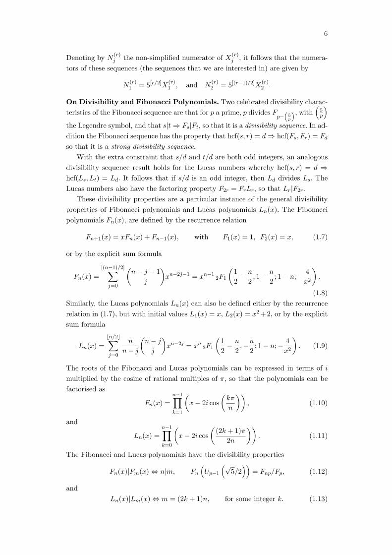
Denoting by N(r)j the non-simplified numerator of X
(r)j , it follows that the numera-
tors of these sequences (the sequences that we are interested in) are given by
N(r)1 = 5[r/2]X
(r)1 , and N
(r)2 = 5[(r−1)/2]X
(r)2 .
On Divisibility and Fibonacci Polynomials. Two celebrated divisibility charac-
teristics of the Fibonacci sequence are that for p a prime, p divides Fp−
(5p
), with (5p
)the Legendre symbol, and that s|t⇒ Fs|Ft, so that it is a divisibility sequence. In ad-
dition the Fibonacci sequence has the property that hcf(s, r) = d⇒ hcf(Fs, Fr) = Fd
so that it is a strong divisibility sequence.
With the extra constraint that s/d and t/d are both odd integers, an analogous
divisibility sequence result holds for the Lucas numbers whereby hcf(s, r) = d ⇒hcf(Ls, Lt) = Ld. It follows that if s/d is an odd integer, then Ld divides Ls. The
Lucas numbers also have the factoring property F2r = FrLr, so that Lr|F2r.
These divisibility properties are a particular instance of the general divisibility
properties of Fibonacci polynomials and Lucas polynomials Ln(x). The Fibonacci
polynomials Fn(x), are defined by the recurrence relation
Fn+1(x) = xFn(x) + Fn−1(x), with F1(x) = 1, F2(x) = x, (1.7)
or by the explicit sum formula
Fn(x) =
[(n−1)/2]∑j=0
(n− j − 1
j
)xn−2j−1 = xn−1
2F1
(1
2− n
2, 1− n
2; 1− n;− 4
x2
).
(1.8)
Similarly, the Lucas polynomials Ln(x) can also be defined either by the recurrence
relation in (1.7), but with initial values L1(x) = x, L2(x) = x2+2, or by the explicit
sum formula
Ln(x) =
⌊n/2⌋∑j=0
n
n− j
(n− j
j
)xn−2j = xn 2F1
(1
2− n
2,−n
2; 1− n;− 4
x2
). (1.9)
The roots of the Fibonacci and Lucas polynomials can be expressed in terms of i
multiplied by the cosine of rational multiples of π, so that the polynomials can be
factorised as
Fn(x) =n−1∏k=1
(x− 2i cos
(kπ
n
)), (1.10)
and
Ln(x) =
n−1∏k=0
(x− 2i cos
((2k + 1)π
2n
)). (1.11)
The Fibonacci and Lucas polynomials have the divisibility properties
Fn(x)|Fm(x) ⇔ n|m, Fn
(Up−1
(√5/2))
= Fnp/Fp, (1.12)
and
Ln(x)|Lm(x) ⇔ m = (2k + 1)n, for some integer k. (1.13)

7
The Fibonacci sequence is then obtained by setting x = 1, so that Fn = Fn(1),
and similarly for the Lucas sequence with Ln = Ln(1). Taking x ∈ {2, 3, 4, . . . },then produces one possible definition of higher dimensional Fibonacci and Lucas
sequences which obey the divisibility properties as stated.
For the interlacing Fibonacci sequences of dimension two, and r ≥ 0, we have
N(2r)1 = L2r, N
(2r+1)1 = −F2r+1, N
(2r+1)2 = L2r+1 and N
(2r)2 = −F2r.
Using the methodology of [21] (Chapter VI), it can be shown that many of the
divisibility properties of the Fibonacci and Lucas sequences transfers to our inter-
lacing sequences, such as if s/d and t/d are both odd integers, then hcf(s, t) = d⇒hcf(N
(s)1 , N
(t)1
)= |N (d)
1 |, and N(2r)2 = N
(r)1 N
(r)2 , and that the sequence N
(r)2 also
forms a divisibility sequence.
2 The Main Results
In order that we may fully state our results we now introduce the polynomials that
are central to our theories.
Definition (Of generating function polynomials). For natural number m, we define
Pm(x), Qm(x), Pm(x), Qm(x) and Vm(x), to be the polynomials of degree m given
by
Pm(x) =
m∑k=0
2m+ 1
2k + 1
(m+ k
2k
)xk, Qm(x) =
m∑k=0
m
k
(m+ k − 1
2k − 1
)xk, (2.1)
Pm(x) =
m∑k=0
(m+ k
2k
)xk, Qm(x) =
m∑k=0
(m+ k + 1
2k + 1
)xk, (2.2)
and
Vm(x) =
m∑k=0
(−1)m+[ k2+m2 ]([k
2 + m2
]k
)xk, (2.3)
where the identity
limk→0
j
k
(j + k − 1
2k − 1
)= 2, (2.4)
ensures that Qm(x) is well defined.
We label the roots of Pm(x), ordered in terms of increasing absolute value, by
µm1, µm2, . . . , µmm, and similarly νm1, νm2, . . . , νmm the ordered m roots of Qm(x),
so that we may write
Pm(x) =
m∏i=1
(x− µmi), Qm(x) =
m∏i=1
(x− νmi), (2.5)
where for i < j, we have |µmi| ≤ |µmj |, and |νmi| ≤ |νmj |.
In Theorem 1 we give simple expressions for the polynomials Pm(x), Qm(x),
Pm(x), Qm(x) and Vm(x), in terms of Chebyshev Sm(x) and Cm(x) polynomials,
and Fibonacci and Lucas polynomials, as well as detailing some of the identities that
exist between them.

8
THEOREM 1. The roots of the equations Pm(x) = 0 and Qm(x) = 0 are real,
simple, negative, contained within the interval [−4, 0], and with the above definitions
for µm,k and νm,k, 1 ≤ k ≤ m, we have
µm,k = ϕm,k−2 = 2 cos
(2πk
2m+ 1
)−2, νm,k = ψm,k−2 = 2 cos
(π(2k − 1)
2m+ 1
)−2.
(2.6)
so that Pm(x) =
m∏k=1
(x+ 2− 2 cos
(2πk
2m+ 1
))=
1√xL2m+1
(√x)=
1√x
(F2m+2(
√x) + F2m(
√x)),
(2.7)
= U2m
(√1 +
x
4
)= S2m
(√x+ 4
)= S2m (2 cos y) , with x = 2 cos 2y−2, (2.8)
and
Qm(x) =
m∏k=1
(x+ 2− 2 cos
(π(2k − 1)
2m
))= L2m
(√x)= F2m+1(
√x)+F2m−1(
√x)
(2.9)
= 2T2m
(√1 +
x
4
)= C2m
(√x+ 4
)= C2m (2 cos y) , with x = 2 cos 2y − 2.
(2.10)
We also have the expressions
Pm(x) =
m∏k=1
(x+ 2 + 2 cos
(2πk
2m+ 1
))= F2m+1
(√x), (2.11)
= U2m
(√−x4
)= S2m
(√−x)= S2m (2i cos y) , with x = 2 cos 2y + 2, (2.12)
Qm(x) =1√xF2m+2
(√x)
(2.13)
and
Vm(x) =m∏k=1
(x− 2 cos
(2πk
2m+ 1
))=
m∑k=0
(−1)m+[ k2+m2 ]([k
2 + m2
]k
)xk (2.14)
= U2m
(√1 + x/2
2
)= S2m
(√x+ 2
)= S2m (2 cos y) , with x = 2 cos 2y,
(2.15)
the relations
Pm(x) = (−1)mPm(−x− 4), (2.16)
Vm(x) = Pm(x− 2), (2.17)
xPm(−x2) = (−1)m−1Q2m+1(−x− 2), (2.18)
Qm(−x2) = (−1)mQ2m(−x− 2), (2.19)

9
and
Qm(x) =
{Pm1(x)Pm1(x) if m = 2m1 is even,
Qm1+1(x)Qm1(x) if m = 2m1 + 1 is odd(2.20)
along with the integral identity∫ √x
0Pm(t2)dt =
√xPm(x), (2.21)
which yields
Pm(x) = Pm(x) + 2xP ′m(x). (2.22)
THEOREM 2. With Cn(x), the minimal polynomial of 2 cos(πn
), and Θn(x), the
minimal polynomial of 2 cos(2πn
), we have
Pm(x− 2)
Θ2m+1(x)=
{= 1 if 2m+ 1 is a prime number,
∈ Z[x] otherwise.
(2.23)
Qm(x− 2)
C2m(x)=
= 1 if m is a power of 2,
= x if m is an odd prime number,
∈ Z[x] otherwise.
(2.24)
−2Q2m+1(−x− 2)
xC4m+2(x)=
(−1)mPm(−x2)C4m+2(x)
=
{= 1 if 2m+ 1 is a prime number,
∈ Z[x] otherwise.
(2.25)
Qm(−x− 2)
C4m(x)=
(−1)mQm(−x2)C4m(x)
=
{= 1 if m is a power of 2,
∈ Z[x] otherwise.(2.26)
(−1)mPm(−x− 2)
C2m+1(x)=
Vm(x)
C2m+1(x)=
{= 1 if 2m+ 1 is a prime number,
∈ Z[x] otherwise.
(2.27)
COROLLARY. Let ρn(x), be the minimal polynomial of 2 cos(2πn
)− 2, τn(x), be
the minimal polynomial of 2 cos(πn
)− 2, and φn(x), be the minimal polynomial of
−2 cos(2πn
)− 2. Then
Pm(x) =∏
d|2m+1
d≥3
ρd(x), Qm(x) =∏d|m
m/d is odd
τ2d(x), Pm(x) =∏
d|2m+1
d≥3
φd(x),
(2.28)
and
Qm(x) = Pm1(x)Pm1(x) =∏
d|2m1+1
d≥3
ρd(x)φd(x), (2.29)
if m = 2m1, is even, and
Qm(x) = Q2mr(x)r−1∏j=1
Qmj+1(x) = Pm1(x)Pm1(x)r−1∏j=1
Qmj+1(x), (2.30)

10
if m = 2m1 + 1 = 2r+1(2mr + 1)− 1, is odd.
Here we mean that for 1 ≤ j ≤ r− 2, mj = 2mj+1 + 1 and mr−1 = 2mr, so that
m1 + 1
m2 + 1=m2 + 1
m3 + 1= . . . =
mr−2 + 1
mr−1 + 1= 2. (2.31)
THEOREM 3. With P0(x) = 1, P1(x) = 1 + x/3, Q1(x) = 1 + x/2 and Q2(x) =
x2/4+x+1/2, the polynomials Pm(x) and Qm(x) respectively satisfy the three-term
recurrences
Pm+1(x) = (x+ 2)Pm(x)− Pm−1(x), (2.32)
Qm+1(x) = (x+ 2)Qm(x)−Qm−1(x), (2.33)
the ordinary differential equations
x(4 + x)P ′′m(x) + 2(x+ 3)P ′
m(x)−m(m+ 1)Pm(x) = 0, (2.34)
x(4 + x)Q′′m(x) + (2 + x)Q′
m(x) +m2Qm(x) = 0, (2.35)
and for integers k, ℓ, the explicit orthogonality condition∫ 0
−4Pℓ(x)Pk(x)
x1/2
(4 + x)1/2dx = 2πiδℓ k, ℓ, k ≥ 0 (2.36)
∫ 0
−4
Qℓ(x)Qk(x)
x1/2(4 + x)1/2dx = −2πiδℓ k, k = 0, (2.37)
where δℓ k is the Kronecker symbol.
Let
MPm(s) ≡
∫ 0
−4
Pm(x)xs−3/4
(4 + x)3/4dx, Re s > −1/4, (2.38)
MQm(s) ≡
∫ 0
−4
Qm(x)xs−5/4
x3/4(4 + x)3/4dx. (2.39)
Then up to normalization, these Mellin transforms have the form
MPm(s) = (−1)s+5/44s4−m−1Γ(1/4)pm(s)
Γ(s+ 1
4
)Γ(s+ 2m+1
2
) , (2.40)
MQm(s) = (−1)s+3/44s−1Γ(5/4)qm(s)
Γ(s− 1
4
)Γ(s+m)
. (2.41)
COROLLARY. Closed form expressions for the polynomials Pm(x) and Qm(x)
are given by Pm(x− 2) =
2−m−1
((1−
√x+ 2√x− 2
)(x−
√x2 − 4
)m+
(1 +
√x+ 2√x− 2
)(x+
√x2 − 4
)m),
(2.42)
and
Qm(x− 2) = 2−m((x−
√x2 − 4
)m+(x+
√x2 − 4
)m), (2.43)
where for r ≤ [m/2] we have
Pm(x) =r∑
j=0
(−1)r(r
j
)(x+ 2)r−jPm−r−j(x), (2.44)

11
and
Qm(x) =
r∑j=0
(−1)r(r
j
)(x+ 2)r−jQm−r−j(x). (2.45)
We have the orthogonal polynomial relations∫ 0
−4x1/2(4 + x)−1/2Pk(x)(any polynomial of degree < k)dx = 0. (2.46)
∫ 0
−4x−1/2(4 + x)−1/2Qk(x)(any polynomial of degree < k)dx = 0. (2.47)
The polynomial factors of MPm(s) and MQ
m(s) satisfy the functional equations
pn(s) = ±pn(1− s), qn(s) = ±qn(1− s) (2.48)
and have zeros only on the critical line Re s = 1/2.
There has been interest in generalised Fibonacci number sequences for some time
(see for example [24]). We give our interlacing definition below.
Definition (Ofm-dimensional interlacing Fibonacci sequences). Denote by by F(r)j ,
1 ≤ j ≤ m, the rth term in the jth rational interlacing Fibonacci sequence of
dimension m. For the case m = 2, apart from an index shift of one place for the
sequence X(r)1 , these rational sequence terms are identical to those given in the
example of the introduction, so that
F(r+1)1 = X
(r)1 , F
(r)2 = X
(r)2 .
This index shift ensures that in the ratio F(r)2 /F
(r)1 , the powers of 5 cancel.
In the general setting of dimension m, due to the natural representation of the
trigonometric and polynomial formulae (derived later), this alignment of denomina-
tor powers of 2m+1 then holds in all the m dimensional sequences, simplifying the
convergence properties of Theorem 5. In particular, denoting by f(r)j the numerator
of the un-simplified rational sequence term F(r)j , we have
F(r)j
F(r)k
=f(r)j
f(r)k
,
with f(r)j an integer sequence. For a given natural number m, it is the set of m
integer sequences f(r)j , which we refer to as the interlacing Fibonacci sequences of
dimension m. We now give the recurrence definition for the rational interlacing
Fibonacci sequences F(r)j .
Let the matrices of binomial coefficients Bodd and Beven be defined such that
Bodd = (bi,j)m×m, with bi,j = (−1)i+j−1
(2j − 1
j − i
),
and
Beven = (bi,j)m×m, with bi,j = (−1)i+j
(2j
j − i
),
12
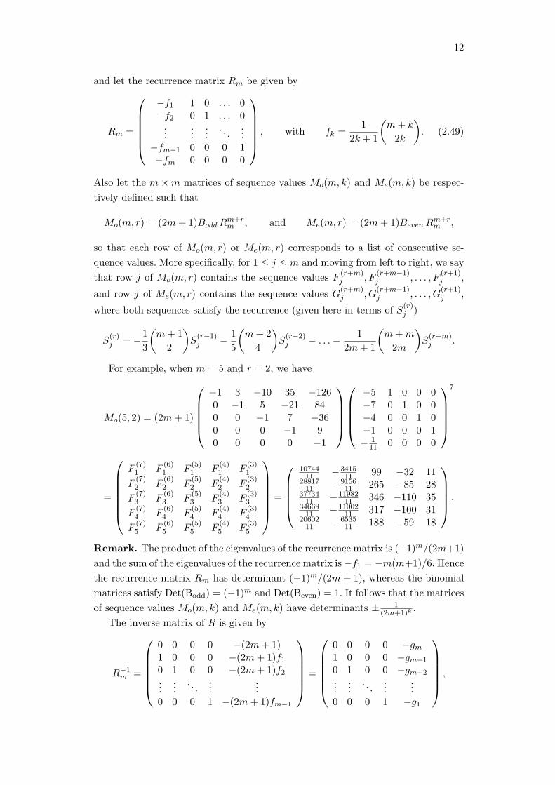
and let the recurrence matrix Rm be given by
Rm =
−f1 1 0 . . . 0−f2 0 1 . . . 0...
......
. . ....
−fm−1 0 0 0 1−fm 0 0 0 0
, with fk =1
2k + 1
(m+ k
2k
). (2.49)
Also let the m ×m matrices of sequence values Mo(m, k) and Me(m, k) be respec-
tively defined such that
Mo(m, r) = (2m+ 1)BoddRm+rm , and Me(m, r) = (2m+ 1)BevenR
m+rm ,
so that each row of Mo(m, r) or Me(m, r) corresponds to a list of consecutive se-
quence values. More specifically, for 1 ≤ j ≤ m and moving from left to right, we say
that row j of Mo(m, r) contains the sequence values F(r+m)j , F
(r+m−1)j , . . . , F
(r+1)j ,
and row j of Me(m, r) contains the sequence values G(r+m)j , G
(r+m−1)j , . . . , G
(r+1)j ,
where both sequences satisfy the recurrence (given here in terms of S(r)j )
S(r)j = −1
3
(m+ 1
2
)S(r−1)j − 1
5
(m+ 2
4
)S(r−2)j − . . .− 1
2m+ 1
(m+m
2m
)S(r−m)j .
For example, when m = 5 and r = 2, we have
Mo(5, 2) = (2m+ 1)
−1 3 −10 35 −1260 −1 5 −21 840 0 −1 7 −360 0 0 −1 90 0 0 0 −1
−5 1 0 0 0−7 0 1 0 0−4 0 0 1 0−1 0 0 0 1− 1
11 0 0 0 0
7
=
F
(7)1 F
(6)1 F
(5)1 F
(4)1 F
(3)1
F(7)2 F
(6)2 F
(5)2 F
(4)2 F
(3)2
F(7)3 F
(6)3 F
(5)3 F
(4)3 F
(3)3
F(7)4 F
(6)4 F
(5)4 F
(4)4 F
(3)4
F(7)5 F
(6)5 F
(5)5 F
(4)5 F
(3)5
=
1074411 −3415
11 99 −32 112881711 −9156
11 265 −85 283773411 −11982
11 346 −110 353466911 −11002
11 317 −100 312060211 −6535
11 188 −59 18
.
Remark. The product of the eigenvalues of the recurrence matrix is (−1)m/(2m+1)
and the sum of the eigenvalues of the recurrence matrix is−f1 = −m(m+1)/6. Hence
the recurrence matrix Rm has determinant (−1)m/(2m + 1), whereas the binomial
matrices satisfy Det(Bodd) = (−1)m and Det(Beven) = 1. It follows that the matrices
of sequence values Mo(m, k) and Me(m, k) have determinants ± 1(2m+1)k
.
The inverse matrix of R is given by
R−1m =
0 0 0 0 −(2m+ 1)1 0 0 0 −(2m+ 1)f10 1 0 0 −(2m+ 1)f2...
.... . .
......
0 0 0 1 −(2m+ 1)fm−1
=
0 0 0 0 −gm1 0 0 0 −gm−1
0 1 0 0 −gm−2
......
. . ....
...0 0 0 1 −g1
,

13
where
gk =2m+ 1
2m+ 1− 2k
(2m− k
k
), so that gk = (2m+ 1)fm−k, (2.50)
and due to the divisibility properties of binomial coefficients, it follows that the
matrices of the first m sequence values,Mo(m, 0) andMe(m, 0), are integer matrices
if and only if 2m+ 1 is a prime number.
Denoting by Rm(x) and R(−1)m (x) the respective characteristic polynomials of Rm
and R−1m , we see that
Rm(x) = −m∑j=0
fm−jxj , R(−1)
m (x) = −(2m+ 1)
m∑j=0
fjxj = −Pm(x),
so that the eigenvalues of the inverse recurrence matrix R−1 are the roots of the
generating function Pm(x) and similarly that the eigenvalues of the recurrence matrix
Rm are the roots of the generating function P (−1)(x) (say) for the inverse recurrence.
THEOREM 4. For natural number m, and 1 ≤ k ≤ m, let F(r)k and G
(r)k be defined
as above. Then for 0 ≤ j ≤ m− 1, we have
F(r)m−j =
j∑k=0
(j + k + 1
2k + 1
)F (r−k)m , G
(r)m−j = −
j∑k=0
(j + k
2k
)F (r−k)m , (2.51)
so that for 1 ≤ k ≤ m, each of the sequence terms in the sequence {F (r)k }∞r=1 can
be expressed as a linear combination of terms from the sequence {F (r)m }∞r=1, whose
coefficients are binomial coefficients, where we note that F(r)m = −G(r)
m for all r ∈ Z.The generating functions for F
(r)m−j and G
(r)m−j are given by
∞∑r=0
F(r)m−jx
r =(2m+ 1)Qj(x)
Pm(x),
∞∑r=0
G(r)m−jx
r = −(2m+ 1)Pj(x)
Pm(x), (2.52)
so that the sum of the numerator coefficients of each generating function is a Fi-
bonacci number.
Inverting the expressions for F(r)j and G
(r)j in (2.51), we obtain
F(r)j+1 =
j∑k=0
2j + 1
2k + 1
(j + k
2k
)F
(r−k)1 , 0 ≤ j ≤ m− 1, (2.53)
and
G(r)j =
j∑k=0
j
k
(j + k − 1
2k − 1
)F
(r−k)1 , 1 ≤ j ≤ m− 1. (2.54)
COROLLARY. With the r index shifted one place to agree with the sequence def-
inition, we have
F (r)m = −G(r)
m = −m∑k=1
2m+ 1
µrmk
∏j =k(µmk − µmj)
(2.55)

14
= −(2m+1)m∑k=1
(2 cos
(2πk
2m+ 1
)− 2
)−r∏j =k
(2 cos
(2πk
2m+ 1
)− 2 cos
(2πj
2m+ 1
))−1
,
(2.56)
F(r)1 = µ1−r
m 1 + . . .+ µ1−rmm =
m∑k=1
(2 cos
(2πk
2m+ 1
)− 2
)1−r
, (2.57)
and
F(r)j+1 =
m∑t=1
(µmt)1−r Pj (µmt) =
m∑t=1
(µmt)1−r
j∏k=1
(µmt − µj k)
=m∑t=1
(µmt)1−r
j∏k=1
(ϕmt − ϕj k) =m∑t=1
(µmt)1−r S2j
(2 cos
(πt
2m+ 1
))(2.58)
= (−1)r−1m∑t=1
2 sin(π(2j+1)t2m+1
)(2 sin
(πt
2m+1
))2r−1 =m∑t=1
(µmt)1−r Vj (ϕmt) ,
and
G(r)j =
m∑t=1
(µmt)1−rQj (µmt) =
m∑t=1
(µmt)1−r
j∏k=1
(µmt − νj k)
=
m∑t=1
(µmt)1−r C2j
(2 cos
(πt
2m+ 1
))= (−1)r−1
m∑t=1
2 cos(π(2j)t2m+1
)(2 sin
(πt
2m+1
))2r−2 . (2.59)
Remark (To Theorem 4). In the setting of [9], there exists an additional sequence
G(r)0 , thus bringing the total number of sequences F
(r)j and G
(r)j to n = 2m+1, and
which satisfies the relation
G(r)0 = 2F
(r)1 = −2
m∑k=1
G(r)k . (2.60)
Hence, this sequence G(r)0 also obeys the recurrence relation Rm, and we can write
2G(r)j = −
j∑k=0
j
k
(j + k − 1
2k − 1
)2G
(r−k)0 , 1 ≤ j ≤ m− 1. (2.61)
We also note the link to Toeplitz determinants, described in Lemma 6.1 of [9], which
enables us to write
F (r)m = −G(r)
m = −r−1∑k=0
fr−kF(k)m (2.62)
= (−1)r
∣∣∣∣∣∣∣∣∣∣∣∣∣
f1 1 0 0 . . . 0f2 f1 1 0 . . . 0f3 f2 f1 1 . . . 0...
......
.... . .
...fr−1 fr−2 fr−3 fr−4 . . . 1fr fr−1 fr−2 fr−3 . . . f1
∣∣∣∣∣∣∣∣∣∣∣∣∣, (2.63)

15
so that by (2.51) the F(r)j can be written as linear combinations of Toeplitz deter-
minants. For example F(r)1 has the determinant form
F(r)1 = (−1)r+m−1
∣∣∣∣∣∣∣∣∣∣∣∣∣∣∣∣
(m1
)1 0 0 0 . . . 0(
m+13
)f1 1 0 0 . . . 0(
m+25
)f2 f1 1 0 . . . 0(
m+37
)f3 f2 f1 1 . . . 0
......
......
.... . .
...(m+r−12r−1
)fr−1 fr−2 fr−3 fr−4 . . . 1(
m+r2r+1
)fr fr−1 fr−2 fr−3 . . . f1
∣∣∣∣∣∣∣∣∣∣∣∣∣∣∣∣.
Hence for r ∈ N, the sequence terms F(r)j , 1 ≤ j ≤,m, are rational numbers corre-
sponding to a rational multiple of either the r or the (r + 1)-dimensional volume of
the simplex with vertex coordinates given by the row entries of the determinant.
Example (Three-dimensional interlacing case). Let F(r)1 , F
(r)2 and F
(r)3 be the rth
terms of the three rational interlacing Fibonacci sequences, with r = 1, 2, 3, 4, . . .,
and F(1)1 = 3, F
(2)1 = −2, and F
(3)1 = 2, etc, as detailed below, and thereafter
F(r)j = −2F
(r−1)j − F
(r−2)j − 1
7F
(r−3)j .
Then the generating functions and first few terms of these three rational series are
given by:
F(r)1 :
7(x2 + 4x+ 3
)x3 + 7x2 + 14x+ 7
{3,−2, 2,−17
7,22
7,−29
7,269
49,−−357
49,474
49,−4406
343. . .
},
F(r)2 :
7(x+ 2)
x3 + 7x2 + 14x+ 7
{2,−3, 4,−37
7,49
7,−65
7,604
49,−802
49,1065
49,−9900
343. . .
},
F(r)3 :
7
x3 + 7x2 + 14x+ 7
{1,−2, 3,−29
7,39
7,−52
7,484
49,−643
49,854
49,−7939
343. . .
}.
The corresponding integer interlacing Fibonacci sequence terms of dimension 3, f(r)1 ,
f(r)2 and f
(r)3 , can then be obtained from the un-simplified numerators of the rational
sequence terms.
THEOREM 5 (Convergence theorem). Define the m-dimensional vectors F(r)m and
Ψm such that F(r)m =F (r)
m−1
F(r)m
,F
(r)m−3
F(r)m−1
, . . . ,F
(r)m−2r+1
F(r)m−r+1
, . . .−F (r)
1
F(r)[m/2]+1
, . . . ,−F (r)
2r−m
F(r)m−r+1
, . . . ,−F (r)
m
F(r)1
=
f (r)m−1
f(r)m
,f(r)m−3
f(r)m−1
, . . . ,f(r)m−2r+1
f(r)m−r+1
, . . .−f (r)1
f(r)[m/2]+1
, . . . ,−f (r)2r−m
f(r)m−r+1
, . . . ,−f (r)m
f(r)1
, (2.64)
and
Ψm = (ϕm1, ϕm2, ϕm3, . . . , ϕmm) .

16
We have limr→∞F(r)m =(
µm (m−1) − µm (m−2)
µmm − µm (m−1), . . . ,
µm (m−2r+1) − µm (m−2r)
µm (m−r+1) − µm (m−r), . . .
−(µm 1 − µm 0)
µm ([m/2]+1) − µm [m/2], . . .
. . . ,−(µm (2r−m) − µm (2r−m−1)
)µm (m−r+1) − µm (m−r)
, . . . ,−(µmm − µm (m−1)
)µm 1 − µm 0
)= Ψm, (2.65)
or equivalently limr→∞F(r)m =(
ϕm (m−1) − ϕm (m−2)
ϕmm − ϕm (m−1), . . . ,
ϕm (m−2r+1) − ϕm (m−2r)
ϕm (m−r+1) − ϕm (m−r), . . .
−(ϕm 1 − ϕm 0)
ϕm ([m/2]+1) − ϕm [m/2], . . .
. . . ,−(ϕm (2r−m) − ϕm (2r−m−1)
)ϕm (m−r+1) − ϕm(m−r)
, . . . ,−(ϕmm − ϕm (m−1)
)ϕm 1 − ϕm 0
)= Ψm, (2.66)
so that the entries in the vector F(r)m are rational convergents to 2 cos
(2πkn
), and
limr→∞
(x2 −
F(r)m−1
F(r)m
x+ 1
)× . . .×
(x2 +
F(r)m
F(r)1
x+ 1
)
= limr→∞
(x2 −
f(r)m−1
f(r)m
x+ 1
)× . . .×
(x2 +
f(r)m
f(r)1
x+ 1
)= x2m + x2m−1 + . . .+ x+ 1.
Example. When m = 3, so that n = 7, then
limr→∞
F(r)2
F(r)3
= limr→∞
f(r)2
f(r)3
=µ3 2 − µ3 1µ3 3 − µ3 2
=ϕ3 2 − ϕ3 1ϕ3 3 − ϕ3 2
= ϕ3 1 = 2 cos2π
7.
Or from a cyclotomic perspective, in consideration of the Euclidean distance regard-
ing the 20th convergent when m = 5, we have∣∣∣F(20)5 −Ψ5
∣∣∣ = ∣∣∣∣∣(f(20)4
f(20)5
,f(20)2
f(20)4
,−f(20)1
f(20)3
,−f(20)3
f(20)2
,−f(20)5
f(20)1
)− (ϕ5 1, ϕ5 2, ϕ5 3, ϕ5 4, ϕ5 5)
∣∣∣∣∣=∣∣( 42951850444254470
25528481467235249, 3568568702151113342951850444254470
,− 443437005607040815579436796165461
,− 4673831038849638335685687021511133
,− 2552848146723524913303110168211224)
−(2 cos
(2π
11
), 2 cos
(4π
11
), 2 cos
(6π
11
), 2 cos
(8π
11
), 2 cos
(10π
11
))∣∣∣∣< 9.99226× 10⁻¹⁴.
This yields(x2 − F
(20)4
F(20)5
x+ 1
)(x2 − F
(20)2
F(20)4
x+ 1
)(x2 +
F(20)1
F(20)3
x+ 1
)(x2 +
F(20)3
F(20)2
x+ 1
)(x2 +
F(20)5
F(20)1
x+ 1
)−(x10 + x9 + x8 + x7 + x6 + x5 + x4 + x3 + x2 + x+ 1
)= −1.4820×10⁻¹³x+1.1038×10−20x2−2.9641×10−13x3+2.2074×10−20x4−2.9641×10−13x5
+2.2074× 10−20x6 − 2.9641× 10−13x7 + 1.1038× 10−20x8 − 1.4820× 10−13x9.
With this example in mind, the question of the rates of convergence achieved with
these sequences could well be of interest.

17
Definition (Of Fleck’s and Weisman’s congruences). Let p be a prime and a be an
integer. In 1913 A. Fleck discovered that∑q≡a (mod p)
(−1)q(N
q
)≡ 0
(mod p
⌊N−1p−1
⌋), (2.67)
for all positive integers N > 0. In 1977 C. S. Weisman [23] extended Fleck’s congru-
ence to obtain
∑q≡a (mod pα)
(−1)q(N
q
)≡ 0
(mod p
⌊N−pα−1
ϕ(pα)
⌋), (2.68)
where α, N are positive integers ≥ 0, N ≥ pα−1, ϕ denotes the Euler totient function
and ⌊.⌋ is the usual floor function. When α = 1 it is clear that (2.68) reduces to
(2.67).
We define the Fleck numbers, F(N, a (mod n)), to be the numbers generated by
the generalised sum in (2.67) and (2.68), such that
F(N, a (mod n)) =∑
q≡a (mod n)
(−1)q(N
q
). (2.69)
These sums have many well known properties [18] such as
nF(N, a (mod n)) =
N∑k=0
(−1)k(N
k
) ∑γn=1
γk−a =∑γn=1
γ−a(1− γ)N , (2.70)
from which we can deduce the recurrence relation
F(N + 1, a (mod n)) = F(N, a (mod n))−F(N, (a− 1) (mod n)). (2.71)
By the modular definition of the sum in (2.69) we can also deduce that
F(N, a (mod n)) = F(N, (a+ n) (mod n)). (2.72)
THEOREM 6. Let r be a non-negative integer and m be a natural number, so that
n = 2m + 1, is odd. Then the numbers in the sequences F(−r)j and G
(−r)j are given
by the alternating binomial sums
F(−r)j = n
∞∑a=−∞
(−1)r+j+a
(2r + 1
r + j + an
)= nF(2r + 1, (r + j) (mod n)), (2.73)
G(−r)j = n
∞∑a=−∞
(−1)r+j+1+a
(2r + 2
r + j + 1 + an
)= nF(2r + 2, (r + j + 1) (mod n)),
(2.74)
and so satisfy Weisman’s Congruence, when n is a prime power.

18
COROLLARY. With gr defined as in (2.50), the sequence terms F(−r)j , r ≥ 0,
1 ≤ j ≤ m, can also be expressed as linear combinations of Toeplitz determinants,
so that F(−r)m = (−1)r(2m+ 1)×∣∣∣∣∣∣∣∣∣∣∣∣∣
g1 1 0 0 . . . 0g2 g1 1 0 . . . 0g3 g2 g1 1 . . . 0...
......
.... . .
...gr1−1 gr−2 gr−3 gr−4 . . . 1gr gr−1 gr−2 gr−3 . . . g1
∣∣∣∣∣∣∣∣∣∣∣∣∣= −nF(2r + 1, (r +m) (mod n)).
In the terminology of Lemma 3.1 of [10], each sequence term F(−r)j can be expressed
as either a minor corner lattice (MCL) determinant or a half-weighted MCL deter-
minant. This is an analogous result for the determinant expressions of F(r)j , r ≥ 0,
described in the Remark to Theorem 4, and it follows that for allr ∈ Z, the sequence
terms F(r)j , 1 ≤ j ≤,m, relate to the d-dimensional volume of some simplex.
The Fleck numbers can be written as −nF(2r + 1, (r + j) (mod n)) =
m∑t=1
(µmt)r+1 Pj−1 (µmt) =
m∑t=1
(µmt)r+1
j−1∏k=1
(µmt − µ(j−1) k
)(2.75)
=
m∑t=1
(µmt)r+1
j−1∏k=1
(ϕmt − ϕ(j−1) k
)=
m∑t=1
(µmt)r+1 Vj−1 (ϕmt) . (2.76)
Similar expressions exist relating the sequence terms G(−r)j to the Fleck numbers
F(2r + 2, (r + j + 1) (mod n)), formed from the even rows of Pascals triangle.
Example. When m = 5, so n = 11, and r = 8, we have
F(−8)5 = 11
∞∑a=−∞
(−1)8+5+a
(17
8 + 5 + 11a
)= 11
∞∑a=−∞
(−1)a(
17
2 + 11a
)= −(2m+1)×
∣∣∣∣∣∣∣∣2m+ 1 1 0 0
(m− 1)(2m+ 1) 2m+ 1 1 013(m− 2)(2m− 3)(2m+ 1) (m− 1)(2m+ 1) 2m+ 1 1
16(m− 3)(m− 2)(2m− 5)(2m+ 1) 1
3(m− 2)(2m− 3)(2m+ 1) (m− 1)(2m+ 1) 2m+ 1
∣∣∣∣∣∣∣∣m=5
= −1
6(m+ 3)(m+ 4)(2m+ 1)2(2m+ 7)
∣∣∣∣m=5
= −11∗2244 = 11F(17, 2 ( mod 11)) = −112×204
=
5∑t=1
(µ5 t)9 P4 (µ5 t) =
5∑t=1
(µ5 t)9
4∏k=1
(µ5 t − µ4 k)
=
5∑t=1
(µ5 t)9
4∏k=1
(ϕ5 t − ϕ4 k) =
5∑t=1
(µ5 t)9 V4 (ϕ5 t) .
Remark. The relations here all fundamentally stem from the recurrence polynomial
Pm(x) and its inverse recurrence, where the powers of xk are replaced with xm−k.

19
The sequence terms at negative indices then correspond to (2m + 1) times the
Fleck numbers using the odd modulus (2m + 1). It is worth noting that we can
construct a similar family of sequences using the recurrence Qm(x), and its inverse
recurrence, resulting in sequences terms which at negative indices correspond to
(2m) times the Fleck numbers obtained using the even modulus (2m).
In Theorem 7 we establish geometric relations between the sequence terms F(r)j
and G(r)j and the side lengths and ratios of side lengths of the regular n-gon inscribed
in the unit circle.
THEOREM 7. For natural number m, let n = 2m+1 be odd, and vn 0, . . . vn (n−1)
be the n vertices of the regular n-gon Hn, inscribed in the unit circle. Let dn r be the
distance from vertex vn 0, to vertex vn r, so that dn 1 = 2 sin (π/n) is the side length
of Hn, dnk = 2 sin ((πk)/n) is the length of the kth diagonal of Hn, and dnn = 0, so
that we may work (mod n) the subscripts.
Define ∇nk to be the ratio of the kth diagonal to the side length, so that ∇nk =
dnk/dn 1. Then we have
∇n (k+1) −∇n (k−1) = Sk
(2 cos
(πn
))= 2 cos
(kπ
n
)(2.77)
∇nk∇n ℓ =
ℓ−1∑j=0
∇n (k−ℓ+2j+1), dnkdn ℓ = dn 1
ℓ−1∑j=0
dn (k−ℓ+2j+1), (2.78)
where we take (k − ℓ+ 2j + 1) (mod n). Hence
F(r)j+1 = (−1)r−1
m∑t=1
dn (2j+1)t
d2r−1n t
= (−1)r−1m∑t=1
∇n (2j+1)t
d2r−2n t
, (2.79)
and
G(r)j = (−1)r−1
m∑t=1
dn (2j+1)t − dn (2j−1)t
d2r−1n t
(2.80)
= (−1)r−1m∑t=1
∇n (2j+1)t −∇n (2j−1)t
d2r−2n t
= F(r)j+1 − F
(r)j . (2.81)
COROLLARY. For n = 2m + 1 an odd integer with m ≥ 1, the numbers defined
by the sum over t = 1, 2, . . . ,m of the (2jt+ t)th diagonal (mod n) of the unit n-gon
Hn, divided by the (2r − 1)th power of the side length of Hn, can be written as a
rational number, with denominator n([(r−1)/m]), r ∈ Z.These numbers are the sequence numbers F
(r)j+1 of the higher-dimensional inter-
lacing Fibonacci sequences described in this paper, and so obey an m-term recurrence
and at negative values of r, correspond to integers which are the Fleck numbers mul-
tiplied by n. Their ratios, as ordered in Theorem 5, will also converge to the cosines
ϕmk, with k = 1, 2, . . .m.
We now define the integer interlacing Fibonacci sequences of dimension m

20
THEOREM 8 (Integer sequence theorem). Let p1, p2, . . . pt be all the prime factors
of n = 2m + 1, so that the number p1 × p2 × . . . × pt is the radical rad(n), of the
integer n. Then for 1 ≤ j ≤ m, and r > 0, the sequences defined by
f(r)j =
(t∏
i=1
p⌊ r−1
m ⌋i
)F
(r)j = (rad(n))⌊
r−1m ⌋ F (r)
j ,
are integer sequences, which we refer to as the integer interlacing Fibonacci sequences
of dimension m.
For F(r)j with r ≤ 0, and n a composite number, define f
(r)j = F
(r)j , and when
n = pα is a prime power, define
f(r)j =
(p−α−
⌊−2r+1−pα−1
pα−pα−1
⌋)F
(r)j .
Then for n a composite number we have that the sequence terms f(r)j , r = 0,−1,−2,−3, . . .,
are the Fleck numbers, and when n = pα is a prime power, we have that the sequence
terms f(r)j are the Fleck quotients discussed in [18].
COROLLARY. We have that any expressions involving ratios of the rational se-
quence terms F(r)j , for different values of j, can be replaced with the ratios of the
integer sequence terms f(r)j .
We also have that when n = p, a prime number, then{p⌊
r−1m ⌋F (r)
j
}+∞
r=−∞={f(r)j
}+∞
r=−∞.
Example.
j/r −6 −5 −4 −3 −2 −1 0 1 2 3 4 5 6 7 8
1 −35 66 −18 5 −10 3 −1 3 −2 2 −17 22 −29 269 −3572 26 −47 12 −3 5 −1 0 2 −3 4 −37 49 −65 604 −8023 −13 22 −5 1 −1 0 0 1 −2 3 −29 39 −52 484 −643
We give the table for the integer sequence f(r)j , when m = 3, and r ∈ [−6, 8].
Remark (to Theorem 8). It is the case that the p-adic structure of the rational
sequence terms F(r)j , at negative indices, follows a very different pattern to the one
at positive indices. In particular, to clear fractions at positive indices we simply use
powers of the radical given by [(r− 1)/m], whereas for negative indices we can only
remove “excess” powers of n when n is a prime power pα. This discrepancy poses
the question as to whether there is a pattern involving the positive index sequence
terms if n contains prime powers and leads us to the following conjecture.
CONJECTURE. If n = 2m+ 1 = p2, for some odd prime p, then the normalised
integer sequences {f(r)m+1+nk
}∞
r=1, 0 ≤ k ≤ 2m2,
are divisible by further powers of p, with the power increasing with the index r.
Similar pattern seem to hold for higher powers of p.

21
Furthermore, when n = p21p2, with p1 = 2m1 + 1 and p2 = 2m2 + 1 then it
appears to be the case that the terms f(r)m1+m2+nk, (or similar) with k = 0, 1, 2, . . .
have further divisibility properties by the prime p1. It may well be the case that there
exists a concise formula, obtained from the prime powers (≥ 2) which divide n, that
generalises to all the prime powers dividing n, and describing the extra prime factors
contained in these specific sequence terms.
THEOREM 9. The polynomials Pm(x) obey the Christoffel-Darboux formula
n∑m=0
Pm(y)Pm(x) =Pn+1(x)Pn(y)− Pn+1(y)Pn(x)
x− y, (2.82)
the confluent form of which (i.e., for y → x) is
n∑k=0
P 2k (x) = P ′
n+1(x)Pn(x)− Pn+1(x)P′n(x). (2.83)
They also satisfy the relation
dPm(x)
dx=
1
x(4 + x){−(2m− 1)Pm−1(x) + [m(x+ 2)− 1]Pm(x)} , (2.84)
and have the raising and lowering operators
Rm = x(x+ 4)d
dx+m(x+ 2) + x+ 3, (2.85)
Lm = −x(x+ 4)d
dx+m(x+ 2)− 1, (2.86)
such that RmPm(x) = (2m + 3)Pm+1(x), and LmPm(x) = (2m − 1)Pm−1(x). The
ordinary differential equation for Pm(x) can then be written in terms of these oper-
ators.
The polynomials Qm(x) obey the quadratic identity
Q2m(x) =
1
mQ2m(x) +
1
2m2, (2.87)
have the generating function
∞∑m=0
(1/2)m(m− 1)!
Qm(x)rm =1
2R−1(1− r +R)1/2(1 + r +R)1/2, (2.88)
where R = (1− 2r − xr + r2)1/2, and satisfy the differential relation
d
dxQm(x) =
sin[m cos−1(1 + x/2)]√−x(4 + x)
. (2.89)
Remark 1 (to Theorem 9 - Generalized raising operator and Rodrigues’ formula).
It is possible to obtain a generalized Rodrigues’ formula for the polynomials Pm(x),
as we now present. Following the procedure of [2] we put Rm = f1ddxg2 + h, where
h is an arbitrary function and f1 and g2 are functions to be determined. We find
g2(x) = exp
[−∫
h(x)
x(x+ 4)dx
]x(m+3/2)/2(x+ 4)(m+1/2)/2,

22
and
f1(x) =x(x+ 4)
g2(x)= exp
[∫h(x)
x(x+ 4)dx
]x−m/2+1/4(x+ 4)−m/2+3/4.
By way of the iteration Pm+1(x) =1
(2m+3)1
(2m+1) · · ·15 · 1
3 · 11RmRm−1 · · ·R1R0P0(x)
for h = 0 we obtain a generalized Rodrigues’ formula
Pm+1(x) =1
(2m+ 3)!!x−m/2+3/4(x+4)−m/2+5/4 d
dx
(x3/2(x+ 4)3/2
d
dx
)m−1
x3/4(4+x)1/4,
where (2n+ 1)!! = (2n+ 1)(2n− 1) · · · 3 · 1.
Remark 2. The higher-dimensional interlacing Fibonacci numbers F(r)j and their
counterparts G(r)j , appear to obey many identities identities such as
F(r)j+1 − F
(r)j = G
(r)j , G
(r)j+1 −G
(r)j = F
(r−1)j ,
the first of which follows from (2.81) of Theorem 7, with the second deduced in a
similar fashion.
We conjecturally state without proof a number of similar relations, including two
quadratic relations for the cases m = 2 and m = 3. Empirically, it appears to be the
case that for r ≥ 1 we have
m∑j=1
(F
(r)j
)2= ±(2m+ 1)F
(2r)1 ,
(G
(r)0
)2+ 2
m∑j=1
(G
(r)j
)2= ±(2m+ 1)G
(2r)0 ,
F(r)j = −
m∑k=j
G(r)k , G
(r)j =
−2
2m+ 1
m∑k=1
(m+ 1− k)F(r−1)k +
j∑k=1
F(r−1)k ,
F(r)j =
−(m+ 1− j)
2m+ 1
m∑k=1
(2k − 1)F(r−1)k +
m−j∑k=1
k F(r−1)j+k ,
with G(r)0 defined as in the remark to Theorem 4. We also appear to have
G(r)j =
−1
2m+ 1
m∑k=1
k2G(r−1)k +
m−j∑k=1
k G(r−1)j+k ,
as well as quadratic sequence relations
F(r)j =
−1
5F
(1)j F
(r−2)2 + F
(2)j F
(r−1)2 ,
when m = 2, and
F(r)j =
−1
7
(F
(1)j F
(r−3)3 − F
(2)j F
(r−4)3
)− F
(2)j F
(r−3)3 − F
(3)j F
(r−2)3 ,
when m = 3.
These identities can be re-stated in terms of the un-simplified integer numerators
f(r)j of F
(r)j and g
(r)j of G
(r)j , and so the integer interlacing Fibonacci sequences.

23
3 Proof of the Theorems
LEMMA 3.1 (Chebyshev identities). With Tn(x) the Chebyshev polynomial of the
first kind, Un(x) the Chebyshev polynomial of the second kind, as defined in (1.2),
we have
Tn(x) = 2n−1n∏
k=1
(x− cos
((2k − 1)π
2n
)), (3.1)
Un(x) = 2nn∏
k=1
(x− cos
(kπ
n+ 1
)), (3.2)
Un(x) = 2
n∑j odd
Tj(x), n odd, Un(x) = 2
n∑j even
Tj(x)− 1, n even, (3.3)
Un(x) =
[n/2]∑r=0
(−1)r(n− r
r
)(2x)n−2r =
[n/2]∑r=0
(n+ 1
2r + 1
)xn−2r(x2 − 1)r, (3.4)
and
Tn+1(x) = 2xTn(x)− Tn−1(x), 2Tm(x)Tn(x) = Tm+n(x) + T|m−n|(x). (3.5)
Proof of Lemma 2.1. For proofs of the above identities we refer the reader to chap-
ters one and two of [15].
Proof of Theorem 1. For k = 1, 2, . . . ,m, the function cos(
2πk2m+1
)is a decreasing
function of k. It follows that ϕmk is a decreasing function of k, and so in terms of
absolute values we have, µm1 > µm2 > . . . > µmm. A similar argument holds for the
νmk, 1 ≤ k ≤ m, and hence (2.5).
Although it follows from (2.6) that the roots of Pm(x) are simple and lie in the
interval [−4, 0], we demonstrate this by two other methods in order to highlight the
links that exist between Pm(x) and the Legendre and Chebyshev functions .
Method 1. By using manipulations with Pochhammer symbols which we omit,
Pm(x) may be written in terms of the Gauss hypergeometric function 2F1. Letting
Pmn (x) denote the associated Legendre function, in turn Pm(x) may be expressed as
Pm(x) =(2m+ 1)
√π
2
(x+ 4)1/4
(−x)1/4P−1/2m
(1 +
x
2
). (3.6)
The functions P−1/2m (z) are orthogonal on the interval [−1, 1]. With x = 2(z − 1),
it follows from a standard result in the theory of orthogonal polynomials [20] that
the zeros of P−1/2m
(1 + x
2
)are contained in [−4, 0] and simple and hence for Pm(x)
too.
Method 2 It is known that (e.g., [11], p. 64)
P−1/2ν (cosφ) =
√2
π sinφ
sin[(ν + 1/2)φ]
(ν + 1/2).
Then with φ replaced by cos−1 φ and x = 2(φ− 1) it again follows that the zeros of
Pm(x) are in [−4, 0] and simple.

24
Remark. It is then possible to write
P−1/2ν (φ) =
√2
π
(1− φ2)1/4
(ν + 1/2)Uν−1/2(φ),
where Uν−1/2 is the Chebyshev function of the second kind.
To see (2.14) and the first part of (2.7), we have
n∏k=1
(x− 2 cos
(2πk
2n+ 1
))= 2n
n∏k=1
(x
2− cos
(2πk
2n+ 1
))
= 1 + 2
n∑k=1
Tk
(x2
)= Un
(x2
)+ Un−1
(x2
)
= U2n
(√1 + x/2
2
)= Pn(x− 2) = Vn(x), (3.7)
where we have used the relations (3.2), (3.3) and (3.4), of Lemma 2.1.
Hencen∏
k=1
(x+ 2− 2 cos
(2πk
2n+ 1
))
= 1 + 2n∑
k=1
Tk
(x2+ 1)= Un
(x2+ 1)+ Un−1
(x2+ 1)
= U2n
(√1 +
x
4
)= Pn(x), (3.8)
and the result follows. Similar arguments can be used to obtain the first statements
of (2.9) and (2.11).
The latter statements in (2.7), (2.9), (2.11), and that of (2.13), concerning ex-
pressions for Pm(x), Qm(x),Pm(x) and Qm(x) in terms of Fibonacci and Lucas poly-
nomials, can be deduced via binomial relations as follows. We have
1√xL2m+1(
√x) =
1√x
m∑j=0
2m+ 1
2m+ 1− j
(2m+ 1− j
j
)(√x)2m+1−2j
=
m∑j=0
2m+ 1
2m+ 1− j
(2m+ 1− j
j
)xm−j =
m∑j=0
2m+ 1
2j + 1
(m+ j
m− j
)xj
=
m∑j=0
2m+ 1
2j + 1
(m+ j
2j
)xj = Pm(x).
Similarly
L2m(√x) =
m∑j=0
2m
2m− j
(2m− j
j
)(√x)2m−2j
=
m∑j=0
2m
2m− j
(2m− j
j
)xm−j =
m∑j=0
m
j
(m+ j − 1
2j − 1
)xj = Qm(x).

25
For the Fibonacci polynomials we have
F2m+1(√x) =
m∑j=0
(2m− j
j
)(√x)2m−2j
=m∑j=0
(2m− j
j
)xm−j =
m∑j=0
(m+ j
2j
)xj = Pm(x),
and1√xF2m+2(
√x) =
1√x
m∑j=0
(2m+ 1− j
j
)(√x)2m+1−2j
=m∑j=0
(2m+ 1− j
j
)xm−j =
m∑j=0
(m+ j + 1
m− j
)xj
=m∑j=0
(m+ j + 1
2j + 1
)xj = Qm(x).
The generating functions for the Lucas and Fibonacci polynomials are respectively
given by
GL(x, t) =∞∑n=0
Ln(x)tn =
1 + t2
1− t2 − tx, GF (x, t) =
∞∑n=0
Fn(x)tn =
t
1− t2 − tx,
so that tGL(x, t) = (1 + t2)GF (x, t). Hence we have that
Ln(x) = Fn+1(x) + Fn−1(x),
giving
Pm(x) =1√x
[F2m+2(
√x) + F2m(
√x)],
and
Qm(x) = F2m+1(√x) + F2m−1(
√x).
Combining the above expressions with the relation
F2m(x) = Fm(x)Lm(x),
we then obtain
Pm(x)Pm(x) =1√xL2m+1(
√x)F2m+1(
√x) =
1√xF4m+2(
√x) = Q2m(x),
and
Qm+1(x)Qm(x) =1√xL2m+2(
√x)F2m+2(
√x) =
1√xF4m+4(
√x) = Q2m+1(x).
The Chebyshev identities in (2.8), (2.10), (2.12) and (2.15) can be derived directly
from the definition (1.2), with further connections to the Chebyshev polynomials
established via the expression for Pm(x) given by
Pm(x) = Tm(1 + x/2) +√
1 + 4/x sinh[2m csch−1(2/√x)].

26
Substituting −(x+ 2) in the product formula for Pm(x) in (2.7) and comparing
with (2.14), gives us the identity (2.17), and writing
Q2m+1(−(x+ 2)) =
2m+1∏k=1
(−x− 2 cos
(π(2k − 1)
4m+ 2
))
=(−x− 2 cos
(π2
)) m∏k=1
(−x− 2 cos
(π(2k − 1)
4m+ 2
))(−x+ 2 cos
(π(2k − 1)
4m+ 2
))
= (−x)m∏k=1
(x2 − 4 cos2
(π(2k − 1)
4m+ 2
))= (−x)
m∏k=1
(x2 − 2
(1 + cos
(π(2k − 1)
2m+ 1
)))
= (−x)m∏k=1
(x2 − 2− ψmk
)= (−1)m−1 x
m∏k=1
(−x2 + 2− ϕmk
)= (−1)m−1xPm(−x2),
we obtain (2.18). Similar arguments produce (2.16), (2.17), (2.19) and (2.20).
Considering (2.21) we have
∫ √x
0
m∑k=0
(m+ k
2k
)t2kdt = t
m∑k=0
(m+k2k
)t2k
2k + 1
∣∣∣∣∣√x
t=0
=√xPm(x),
and differentiating we obtain (2.22).
Proof of Theorem 2. We recall that the minimal polynomial of an algebraic number
β, is defined to be the monic polynomial of minimal degree, with rational coefficients,
which has β as one of its roots. Such polynomials often exhibit structural properties,
such as Φn(x), the minimal polynomial of a primitive nth root of unity, e(k/n), with
(k, n) = 1, which satisfies
xn − 1 =∏d|n
Φd(x). (3.9)
It was shown in [19] that when n is a prime number p, then the minimal polynomial
Θn(x) of 2 cos (2π/n) is given by Θn(x) = fn(x), with
fn(x) =
[n2]∑
k=0
(−1)k(n− k
k
)xn−2k −
[n+12
]∑k=0
(−1)k(n− k
k − 1
)xn−2k+1,
and that Θn(x)|fn(x) for all n ∈ N. By algebraic manipulation we have
Pm(x− 2) = fm(x),
and hence (2.23). In fact, for p a prime number, we can write
Θp(2x) = 2(p−1)/2Ψp(x),
whereΨn(x) denotes the minimal polynomial of the algebraic number β(n) = cos (2π/n).

27
It was shown by Watkins and Zeitlin [22] that analogous formulae to (3.9) for
Ψn(x) are given by
Tn1+1(x)− Tn1(x) = 2n1∏d|n
Ψd(x), n = 2n1 + 1 is odd, (3.10)
Tn1+1(x)− Tn1−1(x) = 2n1∏d|n
Ψd(x), n = 2n1 is even, (3.11)
from which we can establish the explicit formula
Ψn(x) =
[n/2]∏k=1
(n,k)=1
(x− cos
(2πk
n
)),
so that deg Ψn(x) = 1 if n = 1, 2 and ϕ(n)/2 if n ≥ 3. From this one deduces that
Cn(x), the minimal polynomial of 2 cosπ/n, is given by
C1 = 2Ψ2
(x2
), Cn(x) = 2ϕ(2n)/2Ψ2n
(x2
), n ≥ 2.
It follows that deg Cn(x) = 1 if n = 1 and ϕ(2n)/2 if n ≥ 2, the zeros of Cn(x), n ≥ 2,
are 2 cos(πk/n), with k = 1, ..., n− 1 and (k, 2n) = 1. Hence each of the expressions
in (2.24), (2.25), (2.26) and (2.27) are in Z[x] and equal to 1 for the prime conditions
stated. In fact, for n an odd integer, we have Θn(−x) = (−1)ϕ(2n)/2Cn(x).
When n is a power of 2 we use the identity
22m−2
Ψ2m(x) = 2T2m−2(x),
and the result follows.
For completeness we state the case that n is an odd prime power pm, with
p = 2q + 1, for which we have
2pm−1(p−1)/2Ψpm(x) = 2
q∑j=1
Tpm−1j(x)
+ 1
The Corollary can be deduced either from the relations (2.23), (2.24), (2.25), (2.26)
and (2.27), with x−2 replaced by x, in conjunction with (2.16), (2.17), (2.18), (2.19)
and (2.20), or directly from the properties of Fibonacci and Lucas polynomials. In
particular, for p a prime number, the p th Fibonacci and Lucas polynomials are
irreducible and so their roots are respectively 2i times the real and imaginary parts
of the pth cyclotomic polynomial, except for the root 0 in the Lucas polynomial case
(see for example Koshy [8] 2001, p462).
Proof of Theorem 3. The three term recurrences for Pm(x) and Qm(x) in (2.32) and
(2.33) follow from the Legendre function expression for Pm(x) given in (3.6), and
using [1] [p. 99 or 247 or 295] with α = β = −1/2 the Jacobi polynomial P(α,β)n (x)
relation
Qm(x) =(2m)(m− 1)!
(1/2)mP (−1/2,−1/2)m
(1 +
x
2
).
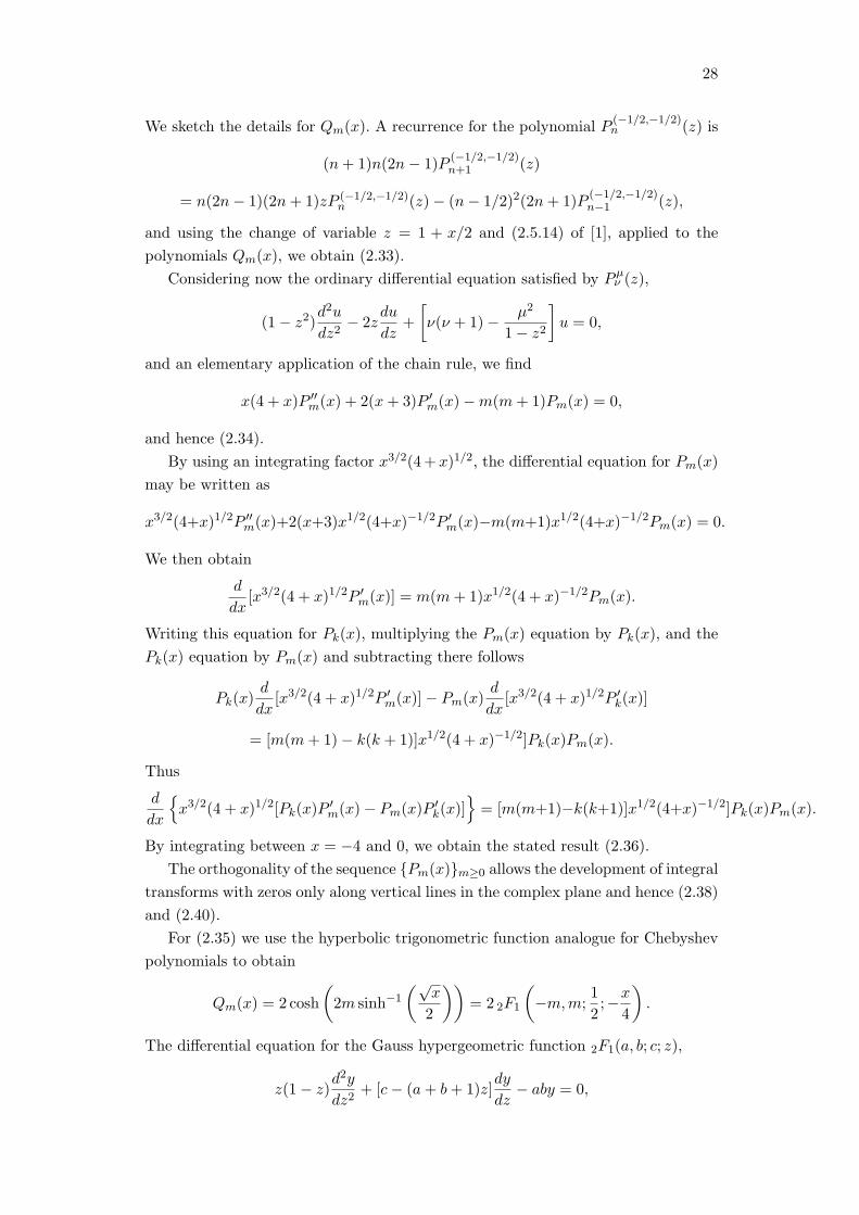
28
We sketch the details for Qm(x). A recurrence for the polynomial P(−1/2,−1/2)n (z) is
(n+ 1)n(2n− 1)P(−1/2,−1/2)n+1 (z)
= n(2n− 1)(2n+ 1)zP (−1/2,−1/2)n (z)− (n− 1/2)2(2n+ 1)P
(−1/2,−1/2)n−1 (z),
and using the change of variable z = 1 + x/2 and (2.5.14) of [1], applied to the
polynomials Qm(x), we obtain (2.33).
Considering now the ordinary differential equation satisfied by Pµν (z),
(1− z2)d2u
dz2− 2z
du
dz+
[ν(ν + 1)− µ2
1− z2
]u = 0,
and an elementary application of the chain rule, we find
x(4 + x)P ′′m(x) + 2(x+ 3)P ′
m(x)−m(m+ 1)Pm(x) = 0,
and hence (2.34).
By using an integrating factor x3/2(4+ x)1/2, the differential equation for Pm(x)
may be written as
x3/2(4+x)1/2P ′′m(x)+2(x+3)x1/2(4+x)−1/2P ′
m(x)−m(m+1)x1/2(4+x)−1/2Pm(x) = 0.
We then obtain
d
dx[x3/2(4 + x)1/2P ′
m(x)] = m(m+ 1)x1/2(4 + x)−1/2Pm(x).
Writing this equation for Pk(x), multiplying the Pm(x) equation by Pk(x), and the
Pk(x) equation by Pm(x) and subtracting there follows
Pk(x)d
dx[x3/2(4 + x)1/2P ′
m(x)]− Pm(x)d
dx[x3/2(4 + x)1/2P ′
k(x)]
= [m(m+ 1)− k(k + 1)]x1/2(4 + x)−1/2]Pk(x)Pm(x).
Thus
d
dx
{x3/2(4 + x)1/2[Pk(x)P
′m(x)− Pm(x)P ′
k(x)]}= [m(m+1)−k(k+1)]x1/2(4+x)−1/2]Pk(x)Pm(x).
By integrating between x = −4 and 0, we obtain the stated result (2.36).
The orthogonality of the sequence {Pm(x)}m≥0 allows the development of integral
transforms with zeros only along vertical lines in the complex plane and hence (2.38)
and (2.40).
For (2.35) we use the hyperbolic trigonometric function analogue for Chebyshev
polynomials to obtain
Qm(x) = 2 cosh
(2m sinh−1
(√x
2
))= 2 2F1
(−m,m;
1
2;−x
4
).
The differential equation for the Gauss hypergeometric function 2F1(a, b; c; z),
z(1− z)d2y
dz2+ [c− (a+ b+ 1)z]
dy
dz− aby = 0,

29
becomes for Qm(x)
d2y
dx2+
(2 + x)
x(4 + x)
dy
dx+
m2
x(4 + x)y = 0,
and the result follows.
In consequence, the family {Qm(x)}m≥1 is orthogonal, and with the integrating
factor√x√4 + x, the differential equation may be written as
d
dx
(√x√4 + x
dy
dx
)=
m2
√x√4 + x
y.
The integrating factor is obtained as the exponential of∫(2 + x)
x(4 + x)dx =
1
2ln[x(4 + x)].
We then obtain the orthogonality relation (2.37) [the steps being omitted]∫ 0
−4
Qm(x)Qk(x)
x1/2(4 + x)1/2dx = −2πiδmk, k = 0.
Accordingly, we have a (generalised) Mellin transform
MQm(s) ≡
∫ 0
−4
Qm(x)xs−5/4
x3/4(4 + x)3/4dx,
of the form (2.41), so that
MQm(s) = (−1)s+3/44s−1Γ(5/4)qm(s)
Γ(s− 1
4
)Γ(s+m)
.
In the Corollary, (2.42) and (2.43) are obtained by solving the recurrences in
(2.32) (2.32), whereas (2.44) and (2.45) arise from iteratively applying the recur-
rences.
The last part of the Corollary follows from properties of orthogonal polynomials.
The proof that the polynomial factors ofMPm(s) andMQ
m(s) satisfy the functional
equations
pn(s) = ±pn(1− s), qn(s) = ±qn(1− s)
and have zeros only on the critical line Re s = 1/2, follows that given in [3]
Proof of Theorem 3. The two identities in (2.51) follow directly from (6.8) and (6.9)
of Lemma 6.2 in [9]. This establishes the numerator polynomials in (2.52). The
denominator polynomials for F(r)m follow from the definitions of Pm(x) and Qm(x),
and hence the result is of the form stated.
With the binomial matrices of initial conditions Mo(m, r) and Me(m, r), so de-
fined, it is possible to invert the identities in (2.51) using a binomial convolution to
obtain (2.53) and (2.54).

30
To see (2.55), we know that Pm(x) factors as Pm(x) =∏m
k=1(x − µm,k). Our
contour integrals from the generating function have the form
1
2πi
∮2m+ 1
zr+1Pm(z)dz.
The contour encloses the origin and at least the interval (−4, 0] of the negative axis.
[In order to contain all of the simple poles of Pm(z) and the higher order pole at the
origin.]
We have that partial fractional decomposition
1
Pm(x)=
m∑k=1
ckx− µmk
,
and we review that ck = 1/P ′m(µmk), the condition that Pm(x) has distinct roots
implying that P ′m(µm,k) = 0. Using the form with lowest common denominator
Pm(x), we have
1
Pm(x)=
m∑k=1
ckx− µmk
=
∑mk=1 ck
∏mj=1,j =k(x− µmj)
Pm(x).
Then 1 =∑m
k=1 ck∏m
j=1,j =k(x − µmj), and, evaluating at µmn, 1 ≤ n ≤ m, gives
1 = cn∏m
j=1,j =n(µmn − µmj) = cnP′m(µmn). Hence cn = 1/P ′
m(µmn).
We have determined that
1
Pm(x)=
m∑k=1
ckx− µmk
=m∑k=1
1
(x− µmk)
1
P ′m(µmk)
wherein P ′m(µmk) =
∏mj=1,j =k(µmk − µmj). Then
1
2πi
∮2m+ 1
zr+1Pm(z)dz =
1
2πi
∮2m+ 1
zr+1
m∑k=1
1
(z − µmk)
1
P ′m(µmk)
dz,
and the residue at z = µmk is given by
(2m+ 1)
µr+1mk
1
P ′m(µmk)
=(2m+ 1)
µr+1mk
1∏mj=1,j =k(µmk − µmj)
.
The pole at the origin gives the F(r)m term generally. Using 2πi times the sum of all
residues gives
F (r)m +
m∑k=1
2m+ 1
µrmk
∏j =k(µmk − µmj)
= 0, r = 1, 2, 3, . . . , (3.12)
and hence the result and (2.56).
The identity F(r)1 = µ1−r
m 1 +µ1−rm 2 + . . .+µ1−r
mm in (2.57) follows similarly to (2.55).
Combining these results with (2.53) and (2.54) then gives
F(r)j+1 =
m∑t=1
j∑k=0
2j + 1
2k + 1
(j + k
2k
)(2 cos
(2πt
2m+ 1
)− 2
)k+1−r
, 0 ≤ j ≤ m− 1.

31
=m∑t=1
(2 cos
(2πt
2m+ 1
)− 2
)1−r j∑k=0
2j + 1
2k + 1
(j + k
2k
)(2 cos
(2πt
2m+ 1
)− 2
)k
=m∑t=1
(2 cos
(2πt
2m+ 1
)− 2
)1−r
Pj
(2 cos
(2πt
2m+ 1
)− 2
)
=m∑t=1
(µmt)1−r Pj (µmt) =
m∑t=1
(µmt)1−r
j∏k=1
(µmt − µjk) ,
and
G(r)j =
j∑k=0
j
k
(j + k − 1
2k − 1
)F
(r−k)1 , 1 ≤ j ≤ m− 1,
=
m∑t=1
j∑k=0
2j
2k
(j + k − 1
2k − 1
)(2 cos
(2πt
2m+ 1
)− 2
)k+1−r
=
m∑t=1
(2 cos
(2πt
2m+ 1
)− 2
)1−r j∑k=0
2j
2k
(j + k − 1
2k − 1
)(2 cos
(2πt
2m+ 1
)− 2
)k
=
m∑t=1
(2 cos
(2πt
2m+ 1
)− 2
)1−r
Qj
(2 cos
(2πt
2m+ 1
)− 2
)
=
m∑t=1
(µmt)1−rQj (µmt) =
m∑t=1
(µmt)1−r
j∏k=1
(µmt − νjk) .
We have thus established (2.58) and (2.59).
LEMMA 3.2 (Fundamental identities). We have
µm1 Pj(µm1) = µm (j+1) − µmj , ∀ j ≥ 0, (3.13)
andµm (m−2r+1) − µm (m−2r)
µm (m−r+1) − µm (m−r)
=ϕm (m−2r+1) − ϕm (m−2r)
ϕm (m−r+1) − ϕm (m−r)= ϕmr, 1 ≤ r ≤
[m2
](3.14)
as well asµm (2r−m) − µm (2r−m−1)
µm (m−r+1) − µm (m−r)
=ϕm (2r−m) − ϕm (2r−m−1)
ϕm (m−r+1) − ϕm (m−r)= −ϕmr,
[m2
]+ 1 ≤ r ≤ m. (3.15)
Proof of Lemma 2.2. From (3.7) and (3.8) in the proof of Theorem 1, we can write
µm 1 Pj(µm 1) = µm 1
(Uj
(cos
(2π
2m+ 1
))+ Uj−1
(cos
(2π
2m+ 1
)))and using the identity
µm 1 = −4 sin2(
π
2m+ 1
),
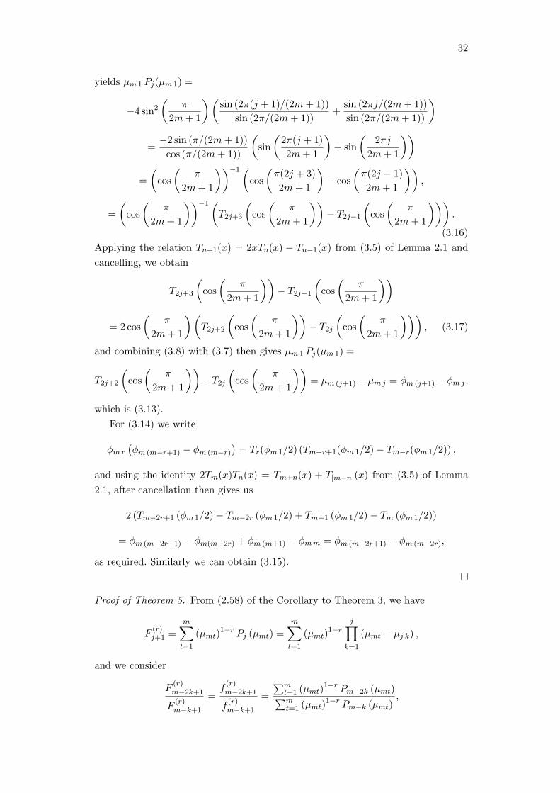
32
yields µm 1 Pj(µm 1) =
−4 sin2(
π
2m+ 1
)(sin (2π(j + 1)/(2m+ 1))
sin (2π/(2m+ 1))+
sin (2πj/(2m+ 1))
sin (2π/(2m+ 1))
)
=−2 sin (π/(2m+ 1))
cos (π/(2m+ 1))
(sin
(2π(j + 1)
2m+ 1
)+ sin
(2πj
2m+ 1
))
=
(cos
(π
2m+ 1
))−1(cos
(π(2j + 3)
2m+ 1
)− cos
(π(2j − 1)
2m+ 1
)),
=
(cos
(π
2m+ 1
))−1(T2j+3
(cos
(π
2m+ 1
))− T2j−1
(cos
(π
2m+ 1
))).
(3.16)
Applying the relation Tn+1(x) = 2xTn(x) − Tn−1(x) from (3.5) of Lemma 2.1 and
cancelling, we obtain
T2j+3
(cos
(π
2m+ 1
))− T2j−1
(cos
(π
2m+ 1
))
= 2 cos
(π
2m+ 1
)(T2j+2
(cos
(π
2m+ 1
))− T2j
(cos
(π
2m+ 1
))), (3.17)
and combining (3.8) with (3.7) then gives µm 1 Pj(µm 1) =
T2j+2
(cos
(π
2m+ 1
))−T2j
(cos
(π
2m+ 1
))= µm (j+1) −µmj = ϕm (j+1) −ϕmj ,
which is (3.13).
For (3.14) we write
ϕmr
(ϕm (m−r+1) − ϕm (m−r)
)= Tr(ϕm 1/2) (Tm−r+1(ϕm 1/2)− Tm−r(ϕm 1/2)) ,
and using the identity 2Tm(x)Tn(x) = Tm+n(x) + T|m−n|(x) from (3.5) of Lemma
2.1, after cancellation then gives us
2 (Tm−2r+1 (ϕm 1/2)− Tm−2r (ϕm 1/2) + Tm+1 (ϕm 1/2)− Tm (ϕm 1/2))
= ϕm (m−2r+1) − ϕm(m−2r) + ϕm (m+1) − ϕmm = ϕm (m−2r+1) − ϕm (m−2r),
as required. Similarly we can obtain (3.15).
Proof of Theorem 5. From (2.58) of the Corollary to Theorem 3, we have
F(r)j+1 =
m∑t=1
(µmt)1−r Pj (µmt) =
m∑t=1
(µmt)1−r
j∏k=1
(µmt − µj k) ,
and we consider
F(r)m−2k+1
F(r)m−k+1
=f(r)m−2k+1
f(r)m−k+1
=
∑mt=1 (µmt)
1−r Pm−2k (µmt)∑mt=1 (µmt)
1−r Pm−k (µmt),

33
by (3.13) of Lemma 2.1.
In the numerator sum above, for large positive values of r, the (µm 1)1−r factor
will dominate as the µmt are ordered in terms of increasing absolute value. Hence, as
r → ∞ the above expression will converge to the ratio of the coefficients of (µm 1)1−r
in the numerator and denominator. Hence we can write
limr→∞
(F
(r)m−2k+1
F(r)m−k+1
)= lim
r→∞
(f(r)m−2k+1
f(r)m−k+1
)= lim
r→∞
((µm 1)
1−r Pm−2k (µm 1)
(µm 1)1−r Pm−k (µm 1)
)
=(µm 1)Pm−2k (µm 1)
(µm 1)Pm−k (µm 1)=ϕm(m−2k+1) − ϕm(m−2k)
ϕm(m−k+1) − ϕm(m−k)= ϕmk
by (3.13) and (3.14) of Lemma 2.1, and the result follows.
Proof of Theorem 6. This is Lemma 4.2 of [9] and the Corollary then follows from
the Theorem.
Proof of Theorem 7. The expression (2.77), follows directly from the definitions given
in the Theorem and (2.78) and (2.79) are a re-statement of the Diagonal Product
Formula given by Steinbach in [16].
Combining the definitions of the diagonal distances and ratios with trigonometric
manipulation of (2.58) and (2.59), which state that
F(r)j+1 = (−1)r−1
m∑t=1
2 sin(π(2j+1)t2m+1
)(2 sin
(πt
2m+1
))2r−1 ,
and
G(r)j = (−1)r−1
m∑t=1
2 cos(π(2j)t2m+1
)(2 sin
(πt
2m+1
))2r−2 .
we obtain (2.80) and (2.81). The Corollary then follows from the previous theorems
stated concerning the sequence terms F(r)j and G
(r)j .
Proof of Theorem 8. The case n = p, a prime number, was proven in Lemma 7.5
of [9]. An expansion of this argument then leads to the deduction that for n =
p1p2 . . . pt, and r at positive integer values, we have that
(rad(n))[r−1m ] F
(r)j ,
is an integer.
By Theorem 6, we know that the sequence terms F(r)J are the Fleck numbers,
and so are already integer values and satisfy Fleck’s and Weisman’s congruences.
The property relating to Fleck quotients when n = (2m + 1) = p, a prime, then
follows from the exponent so that[−2r − 1− pα−1
pα − pα−1
]α=1
=
[−2r − 2
p− 1
]=
[−2r − 2
2m
]=
[−r − 1
m
],
as required.

34
Proof of Theorem 9. The polynomials Pm(x) have the hypergeometric form
Pm(x) = 2F1
(−m,m+ 1;
3
2;−x
4
)=
2
(2m+ 1)√xsinh
[(2m+ 1) sinh−1
(√x
2
)].
Hence their ODE may also be found from that of the 2F1 function.
If we normalize such that Pℓ(x) → Pℓ(x)/√2πi, so that∫ 0
−4P 2k (x)
x1/2
(4 + x)1/2dx = 1,
we obtain the Christoffel-Darboux formula of (2.82)
n∑m=0
Pm(y)Pm(x) =Pn+1(x)Pn(y)− Pn+1(y)Pn(x)
x− y,
and the confluent form of this result (2.83)
n∑k=0
P 2k (x) = P ′
n+1(x)Pn(x)− Pn+1(x)P′n(x),
then follows.
When the relation
(1− z2)dP
−1/2m (z)
dz=
(m− 1
2
)P
−1/2m−1 (z)−mzP−1/2
m (z)
is transformed to the polynomials Pm(x), the result is
dPm(x)
dx=
1
x(4 + x){−(2m− 1)Pm−1(x) + [m(x+ 2)− 1]Pm(x)} ,
which is (2.84). The raising and lowering operators of (2.85) and (2.86) can then be
deduced.
From the application of linear and quadratic transformation of the 2F1 function
we have the following.
Qm(x) =1
m
(1 +
x
4
)m2F1
(−m, 1
2−m;
1
2;
x
x+ 4
)
=(4 + x)m
22m+1m
[(1−
√x
4 + x
)2m
+
(1 +
√x
4 + x
)2m]
=1
m
(1 +
x
4
)−m
2F1
(m,
1
2+m;
1
2;
x
x+ 4
)=
1
m
(1 +
x
4
)1/22F1
(1
2+m,
1
2−m;
1
2;−x
4
)=
1
mcosh
(2m sinh−1
(√x
2
)).
As
Qm(x) =1
m2F1
(−m
2,m
2;1
2;−x
4(4 + x)
),

35
we find that Qm(x) = 12Qm/2[x(4 + x)]. As
Qm(x) =(−1)m
m2F1
(−m,m;
1
2; 1 + x/4
),
we determine that Qm(x) = (−1)mQm(−4− x). Furthermore,
Qm(x) =1
m
√π(2m− 1)!
(m− 1)!Γ(m+ 1/2)
(1 +
x
4
)m2F1
(−m, 1
2−m; 1− 2m;
1
1 + x/4
)=
1
m
√π(2m− 1)!
(m− 1)!Γ(m+ 1/2)
(x4
)m2F1
(−m, 1
2−m; 1− 2m;−4
x
).
With (a)n the Pochhammer symbol, we note the limit for j > 0
lima→−b
(a+ b)j(2a+ 2b)j
=1
2,
[otherwise this ratio is 1 for j = 0]. We then obtain a reduction of Clausen’s identity
for the square of a special 2F1 function,
Q2m(x) =
1
mQ2m(x) +
1
2m2,
which is (2.87)
To see (2.88) we identify Qm(x) in terms of Jacobi polynomials P(α,β)n (x). We
use [1] [p. 99 or 247 or 295] with α = β = −1/2 and obtain
Qm(x) =(m− 1)!
(1/2)mP (−1/2,−1/2)m
(1 +
x
2
).
[We have the Gegenbauer polynomial case of Cλ→0m .]
A generating function for Jacobi polynomials is [1] (p. 298)
F (z, r) =
∞∑n=0
P (α,β)n (z)rn = 2α+βR−1(1− r +R)−α(1 + r +R)−β
where R = (1− 2zr + r2)1/2. Correspondingly we find the generating function
∞∑m=0
(1/2)m(m− 1)!
Qm(x)rm =1
2R−1(1− r +R)1/2(1 + r +R)1/2,
as required, where now R = (1− 2r − xr + r2)1/2.
By [1] (p. 297)
d
dxP (−1/2,−1/2)n (x) =
n
2P
(1/2,1/2)n−1 (x) =
Γ(n+ 1/2) sin(n cos−1 x)√π(n− 1)!
√1− x2
.
We then obtaind
dxQm(x) =
sin[m cos−1(1 + x/2)]√−x(4 + x)
,
which is (2.89).
We note that in terms of Jacobi polynomials Pm(x) can be written as
Pm(x) =m!
(3/2)mP (1/2,−1/2)m
(1 +
x
2
).

36
4 Geometric Interpretations
The geometric relations of Theorem 7 express the higher-dimensional Fibonacci num-
bers in terms of side-lengths and ratios within the unit n-gon. Moreover, for a given
positive integer m, the Remark to Theorem 4 in conjunction with the Corollary to
Theorem 6 demonstrate that these sequence terms correspond to an m-dimensional
volume. Hence when m = 2, we deduce that the Fibonacci and Lucas numbers have
a direct area interpretation. In addition to these geometric properties, there also
exist planar interpretations of Fibonacci numbers and Lucas numbers relating to
continued fractions.
The ratios of consecutive terms of the Fibonacci sequence double as the conver-
gents in the simple continued fraction expansion of the golden ratio −ϕ2 2. Here,
simple means that the numerators in the continued fraction expansion are always 1.
In general, if the sequence of convergents {p0/q0, p1/q1, p2/q2, . . .} to some number
α, is a finite sequence, then α must be rational, and if the series is infinite then α
must be irrational. The convergents pn/qn follow a recurrence relation which can be
concisely written in matrix form such that(pr+1 prqr+1 qr
)=
(pr pr−1
qr qr−1
)(ar+1 11 0
)=
(ar+1pr + pr−1 prar+1qr + qr−1 qr
),
where a0 = [α], and thereafter, a1, a2 . . . are positive integers. For the convergents
to the Golden ratio, we have ar = 1 for all r = 0, 1, 2, . . ..
The simple continued fraction convergents have a geometric interpretation (at-
tributed to Klein), where one considers each convergent pn/qn as the point tn =
(qn, pn) ∈ Z2, so that the numerator of the convergent is the y-value and the de-
nominator its x-value of the point tn in the xy plane.
For a given α ∈ R with sequence of convergents pn/qn, as n = 0, 1, 2, 3, . . . the
lattice points tn approach the line with gradient y = αx in an alternating fashion.
This means that two series of straight lines; one joining the odd numbered lattice
points t2i+1 together and the other joining the even numbered lattice points t2itogether, consist of line segments whose gradients are the convergents to α. To start
both line segment constructions from the axes, we include the point t−1 = (0, 1) on
the y-axis. It follows that the union of the unit axis segments with the two series of
line segments (finite if α ∈ Q, infinite if α ∈ R\Q) forms a closed polygonal body H.
With a bit of thought one can deduce that there do not exist any lattice points
inside the boundary of H, which do not lie on the line y = αx. Therefore H consists
of the union of the two convex hulls H+ and H− constructed from all of the lattice
points lying respectively above and below the line y = αx. This geometric property
represents the fact that the continued fraction algorithm picks up all “good approx-
imations” pn/qn to α. Each line segment si in the convex hull H can be considered
as a multiple of the integer vector vi, defined by the distance between consecutive
lattice points on the line segment.
We give the geometric example for the polygonal hull constructed from the first

37
few terms of the Fibonacci sequence (negative quadrant) and Lucas sequence (pos-
itive quadrant) below. The line of convergence is y = (1 +√5)x/2.
Figure 1: Polygonal hull of the first few terms of the Fibonacci and Lucas sequences.
For increasing terms, the convex hull of the polygonal hull has area (calculated
using Mathematica 8.0){132 ,
392 , 50, 131, 343, 898, 2351, 6155, 16114, 42187
}, which if
one rounds the first term up to 7 and the second term down to 19, gives the sequence
OEIS A100545. This is a Floretion integer sequence relating to Fibonacci numbers
which satisfies the recurrences
an = 3an−1 − an−2, and an−1 = 4F2n + F2n−1 + F2n+1.
It is also linked to√5 via the binomial inversion of the sequence A097924 given by
a(n) =(2√5 + 3)(2 +
√5)n + (2
√5− 3)(2−
√5)n
2√5
.
This series can also be obtained by inverting the sequence A013655, defined by
an = Fn+1 + Ln, further highlighting the connections to the Fibonacci and Lucas
numbers. A slight adjustment to the convex hull produces the secondary sequence of
areas 8, 17, 42, 110, 288, 754, 1974, 5168, 13530, . . ., which if one ignores the first two
terms, corresponds to the sequence (A025169) of twice the even indexed Fibonacci
numbers.
For our two-dimensional integer interlacing Fibonacci sequence we have
limr→∞
f(r+1)1
f(r)1
= limr→∞
f(r+1)2
f(r)2
=ϕ22√5, lim
r→∞
f(r)2
f(r)1
= −ϕ22,
so that the sequence{f(r)2 /f
(r)1 }
}∞
r=1, is a different sequence of convergents to −ϕ22.
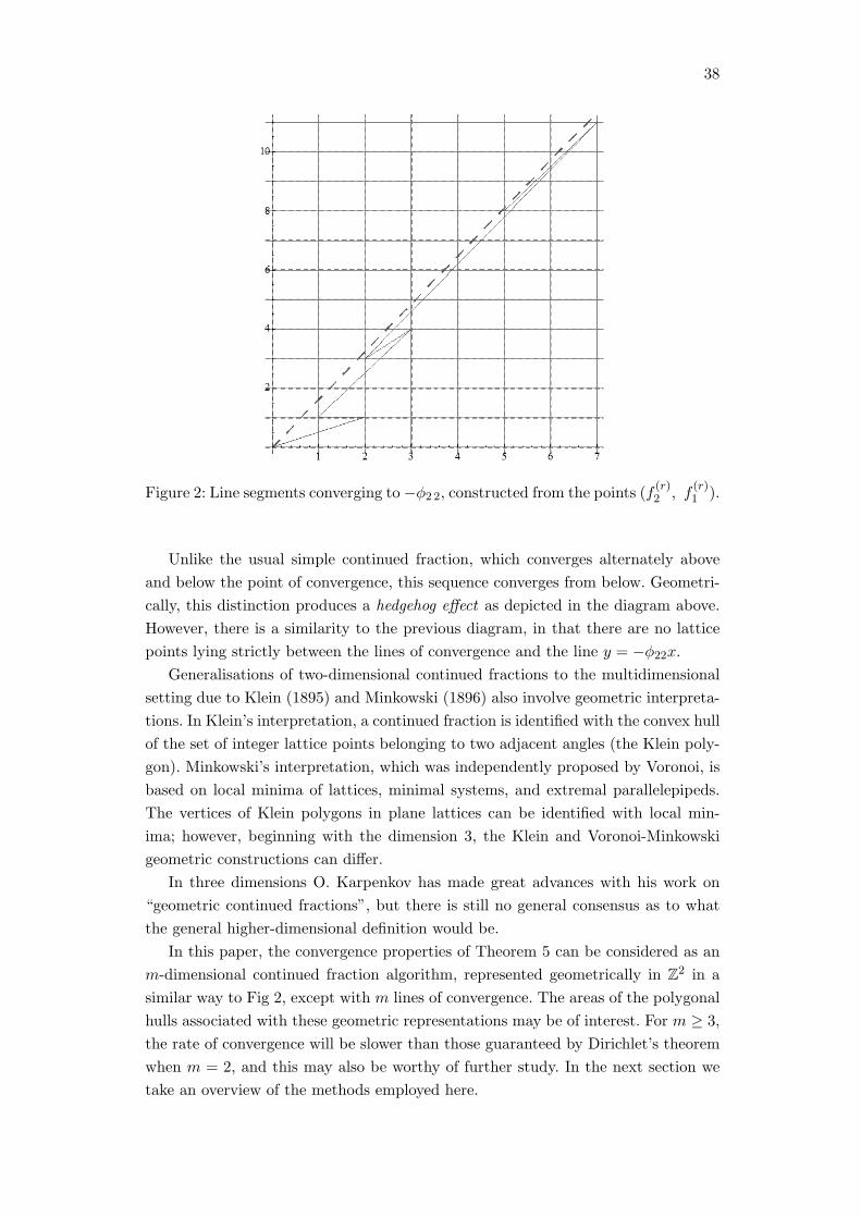
38
Figure 2: Line segments converging to −ϕ2 2, constructed from the points (f(r)2 , f
(r)1 ).
Unlike the usual simple continued fraction, which converges alternately above
and below the point of convergence, this sequence converges from below. Geometri-
cally, this distinction produces a hedgehog effect as depicted in the diagram above.
However, there is a similarity to the previous diagram, in that there are no lattice
points lying strictly between the lines of convergence and the line y = −ϕ22x.Generalisations of two-dimensional continued fractions to the multidimensional
setting due to Klein (1895) and Minkowski (1896) also involve geometric interpreta-
tions. In Klein’s interpretation, a continued fraction is identified with the convex hull
of the set of integer lattice points belonging to two adjacent angles (the Klein poly-
gon). Minkowski’s interpretation, which was independently proposed by Voronoi, is
based on local minima of lattices, minimal systems, and extremal parallelepipeds.
The vertices of Klein polygons in plane lattices can be identified with local min-
ima; however, beginning with the dimension 3, the Klein and Voronoi-Minkowski
geometric constructions can differ.
In three dimensions O. Karpenkov has made great advances with his work on
“geometric continued fractions”, but there is still no general consensus as to what
the general higher-dimensional definition would be.
In this paper, the convergence properties of Theorem 5 can be considered as an
m-dimensional continued fraction algorithm, represented geometrically in Z2 in a
similar way to Fig 2, except with m lines of convergence. The areas of the polygonal
hulls associated with these geometric representations may be of interest. For m ≥ 3,
the rate of convergence will be slower than those guaranteed by Dirichlet’s theorem
when m = 2, and this may also be worthy of further study. In the next section we
take an overview of the methods employed here.

39
5 General Theories
In the preamble to Theorem 3, we defined the m rational sequences F(r)j in terms
of m ×m recurrence matrices, thereby creating a sequence of m ×m matrices. In
Theorem 3, we then obtained explicit expressions for thesem rational sequence terms
whose ordered ratios form our m rational convergents to the algebraic numbers ϕmr,
1 ≤ r ≤ m. The sequence of the m ordered convergents then comprise the sequence
of vectors which converge to the m-dimensional points Ψm, a multi-dimensional
continued fraction.
In this section we consider the underpinning theories behind the recurrence ma-
trices and also the multi-dimensional continued fractions.
5.1 On Minor Recurrence Relations
The k× k minors of the matrix sequence form a set of sequences in their own right,
and we now outline how these k-minor sequences also obey (different) recurrence
relations, for 2 ≤ k ≤ m − 1. The 2 × 2 minors then correspond to the difference
between consecutive convergents after multiplying through by the product of the
two sequence terms which form the denominators of the convergents.
Definition (Fibonacci recurrent polynomials). For 1 ≤ j ≤ m, let the m sequences
{yj n}∞n=1 be defined by an m × m initial value matrix of rational values, and an
m-th order rational linear recurrence given by
yj n = −(a1yj (n−1) + a2yj (n−2) + . . .+ amyj (n−m)
),
so that the denominator of the generating function for the sequence corresponds to
the polynomial
Km(x) =
m∑j=0
ajxj ,
with a0 = 1.
In this general setting we also assume that the system of polynomials Km(x) are
orthogonal, and so satisfy a three-term recurrence, whose measure is supported on
some interval [a, b] ∈ R. This ensures that the roots αm 1, . . . , αmm, of the polynomial
equations Km(x) = 0, are distinct, real algebraic numbers lying in the interval [a, b]
and that these roots interlace. Hence for m > n, there is a root of Km(x) = 0
between any two roots of Kn(x) = 0.
Such systems of recurrence polynomials Km(x), with m = 0, 1, 2, . . ., are said to
be Fibonacci recurrent, where we note that the condition a0 = 1 produces a system
of normalised roots, so that αm 1 × . . . × αmm = 1. We also note that the minimal
polynomials for each of the algebraic numbers αmi divides the polynomial Km(x),
and that∏m
i=1 αmi = 1.
For a given integer value m, the corresponding m×m recurrence matrix Rm can

40
be written as
Rm =
−a1 1 0 0 . . . 0−a2 0 1 0 . . . 0−a3 0 0 1 . . . 0...
......
.... . .
...−am−1 0 0 0 . . . 1−am 0 0 0 . . . 0
,
so that Rm has determinant −am, and characteristic polynomial
Rm(x) = −(am + am−1x+ am−2x2 + . . .+ a2x
m−2 + a1xm−1 + xm) = −
m∑j=0
am−jxj .
Hence as am = 0, the inverse recurrence matrix R−1m exists, and is given by
R−1m =
0 0 0 . . . 0 − 1am
1 0 0 . . . 0 − a1am
0 1 0 . . . 0 − a2am
......
......
. . ....
0 0 1 . . . 0 −am−2
am0 0 0 . . . 1 −am−1
am
,
with generating function denominator
K(−1)m (x) =
1
am
m∑j=0
am−jxj ,
and characteristic polynomial R(−1)m (x) =
− 1
am
(1 + a1x+ a2x
2 + . . .+ am−2xm−2 + am−1x
m−1 + amxm)= − 1
am
m∑j=0
ajxj .
Let λ1, λ2, . . . , λm be the m non-zero, real, algebraic, distinct eigenvalues of the re-
currence matrix Rm (and so the roots of K(−1)m (x)), listed in descending order in
terms of absolute value. Similarly let µ1, µ2, . . . , µm be the ordered distinct eigenval-
ues of the recurrence matrix R−1m (and so the roots of Km(x)), listed in ascending
order in terms of absolute value (of course the eigenvalues µj of the inverse matrix
R−1m are 1/λk, in the reverse order). Then the sequences
Y (j) =(1, λj , λ
2j , λ
3j , . . .
), j = 1, 2, . . .m,
form a basis for the solution space of all possible sequences satisfying the recurrence,
so for any possible starting values. For k such sequences, we require k lots of m
starting values.
Let {y1 j}∞j=0, {y2 j}∞j=0, . . . , {yk j}∞j=0 be k sequences generated by the linear re-
currence so that in matrix form we can write
Y =
y1 0 y1 1 y1 2 y1 3 . . .y2 0 y2 1 y2 2 y2 3 . . ....
......
......
yk 0 yk 1 yk 2 yk 3 . . .
,

41
and consider the sequence formed by successive k × k determinants
Dn =
∣∣∣∣∣∣∣∣∣y1n y1n+1 y1n+2 . . . y1n+k−1
y2n y2n+1 y2n+2 . . . y2n+k−1
......
......
...yk n yk n+1 yk n+2 . . . yk n+k−1
∣∣∣∣∣∣∣∣∣ , n = 0, 1, 2, 3, . . .
The space of all such sequences D(Y ) = (D0, D1, D2, . . .) is spanned by the D’s that
you get by choosing an array Y of the form
Y =
1 γ1 γ21 γ31 . . .1 γ2 γ21 γ32 . . ....
......
......
1 γk γ2k γ3k . . .
,
where the γi are k distinct values chosen from the eigenvalues λj . Here the order of
the rows of Y is irrelevant as we are just looking at how to choose a k element subset
of an m element set. It follows that there are(mk
)ways to choose such an Y , and
from determinant theory the resulting D(Y ) is itself a geometric progression of the
form (C,C∆, C∆2, . . .), where ∆ = γ1γ2 . . . γk. Hence, generically, the space of all
such “minor sequences” must be the solution space of a linear constant coefficient
recurrence of order at most(
mk−1
). We have just proved the following lemma.
LEMMA 5.1. For k ≥ 1, the sequence formed by successive k × k determinants
Dn, as defined above, obeys a linear constant coefficient recurrence of order at most(mk−1
). If the eigenvalues of the minor recurrence matrix all have absolute value less
than 1, then the sequence of k×k determinants Dn will converge to some number α.
Example. We illustrate this lemma with the k minor recurrences corresponding to
the denominator generating function P5(x).{−5,−7,−4,−1,− 1
11
}{7,−19, 29211 ,−
23311 ,
1223121 ,−
356121 ,
63121 ,−
721331 ,
41331 ,−
114641
}{−4,−72
11 ,−6311 ,−
356121 ,−
12231331 ,−
2331331 ,−
29214641 ,−
1914641 ,−
7161051 ,−
11771561
}{1,− 4
11 ,7
121 ,−5
1331 ,1
14641
}{− 1
11
}Here the initial recurrence
F(r)j = −
5∑k=1
1
2k + 1
(5 + k
2k
)F
(r−k)j
is the topmost entry, and the sequence of 2× 2 minors E(r)j obeys the recurrence
E(r)j =
5∑k=1
(−1
11
)k−1 1
11− 2k
(10− k
k
)E
(r−k)j .
In general, for the initial recurrence
F(r)j = −
m∑k=1
1
2m+ 1
(m+ k
2m
)F
(r−k)j

42
we appear to have that the sequence of 2× 2 minors E(r)j obeys the recurrence
E(r)j =
m∑k=1
(−1
2m+ 1
)k−1 1
2m+ 1− 2k
(2m− k
k
)E
(r−k)j ,
when m is odd and
E(r)j = −
m∑k=1
(1
2m+ 1
)k−1 1
2m+ 1− 2k
(2m− k
k
)E
(r−k)j ,
when m is even. The generating functions follow directly from the recurrences and
the recurrence matrix eigenvalues all have absolute value less than 1, so these se-
quences will converge.
Remark. Having established that the sequence of k×k minors, and more specifically
the 2× 2 minors, satisfy a linear recurrence, we look at
{∆n}∞n=0 =
{yr (n+1)
ys (n+1)− yr nys n
}∞
n=0
=
{1
ys nys (n+1)
∣∣∣∣ yr (n+1) yr nys (n+1) ys n
∣∣∣∣}∞
n=0
with
yr n = br 1γn1 + br 2γ
n2 + . . .+ br kγ
nk ,
for some non-zero constants br 1, br 2, . . . br k. Here γ1 is the eigenvalue of the k × k
recurrence matrix with greatest absolute value.
We have
limn→∞
yr nys n
= limn→∞
br 1γn1 + br 2γ
n2 + . . .+ br kγ
nk
bs 1γn1 + bs 2γn2 + . . .+ bs kγnk
=br 1bs 1
,
so that
limn→∞
∆n = 0,
and so the sequence {yr n/ys n}∞n=0 converges, as do the consecutive Fibonacci num-
ber ratios, where the greatest eigenvalue dominates for large values of n.
One can then form sequences in Rk, constructed from these ratios such as{(yr nys n
,y(r+1)n
y(s+1)n, . . . ,
y(r+k−1)n
y(s+k−1)n
)}∞
n=0
,
so that
limn→∞
(yr nys n
,y(r+1)n
y(s+1)n, . . . ,
y(r+k−1)n
y(s+k−1)n
)=
(limn→∞
yr nys n
, limn→∞
y(r+1)n
y(s+1)n, . . . , lim
n→∞
y(r+k−1)n
y(s+k−1)n
)
=
(br 1bs 1
,b(r+1) 1
b(s+1) 1, . . .
b(r+k−1) 1
b(s+k−1) 1
),
and we have a sequence of convergents to the above point in Rk.

43
5.2 On Fibonacci Multi-Dimensional Continued Fractions
The algorithm underpinning the convergence properties of Theorem 5 is a special
case of a multi-dimensional continued fraction. As such it is interesting to take an
overview, in order to try and understand its generality. We give a sequence of steps
below which, for the algebraic points that satisfy the simple Fibonacci convergence
condition, will produce similar results to those of Theorem 5.
In the following definition, we use the word “simple”, as the conditions required
are very strict, and place serious constraints on the interlacing of the zeros of the
system of orthogonal polynomials. It may well be the case that it makes more sense
to relax the conditions, as fundamentally, for a system of Fibonacci recurrent poly-
nomials Km(x), m = 0, 1, 2, 3, . . ., if one expresses each of the rational sequences
derived from the polynomials in power series expansion of the eigenvalues, then one
can always construct m-dimensional rational points of convergence using the ratios
of the coefficients of the eigenvalue with largest absolute value. As such, although
the following conditions give a unique point of convergence in Rm for any polyno-
mial Km(x) that satisfies the condition, it is likely that they do not nearly give the
full picture and that there is a much larger underlying theory to consider. Examin-
ing more closely the convergence properties of the polynomials behind the sequence
terms G(r)j could well be a starting point for such investigations.
Definition (Fibonacci convergent polynomials). Let Km(x) be a system of Fi-
bonacci recurrent polynomials, so that the coefficients of Km(x) are rational num-
bers, and the roots of Km(x), ordering in terms of increasing absolute value, form
an m-tuple of non-zero, real, algebraic numbers α = (αm 1, . . . , αmm) ∈ Rm.
Then we say that the point β is a simply Fibonacci convergent point, if the
following two conditions are satisfied.
(1) The system of m equations in the 2m algebraic variables αm 1, . . . , αmm and
βm 1, . . . , βmm, given by
αm (m−2r+1) − αm (m−2r)
αm (m−r+1) − αm (m−r)= βmr, 1 ≤ r ≤
[m2
], (5.1)
andαm (2r−m) − αm(2r−m−1)
αm(m−r+1) − αm(m−r)= −βmr,
[m2
]+ 1 ≤ r ≤ m, (5.2)
is soluble in Rm, where the point β is an m-tuple of algebraic numbers βmi.
(2) For 1 ≤ j ≤ m, 2 ≤ k ≤ m, and with Aj 1 = αmj − αm (j−1), there exists a set
of algebraic numbers Aj k, such that the m sequences defined by
Y(r)j = (αmj − αm (j−1))α
−rm 1 +Aj 2α
−rm 2 + . . .+Aj mα
−rmm (5.3)
are all rational sequences.
We call the point α the quotient difference convergent for the point β.

44
Remark. In the simplest case, we assume that the m roots of the Fibonacci re-
current polynomial Km(x), are conjugates of some algebraic number, and as such
exhibit similar properties to those of Pm(x) in Lemma 2.2. In this instance, it may
be that we are able to employ the four steps outlined below in order to obtain
a sequence of points in Qm, which converge to some algebraic point in β ∈ Rm.
The coordinates of our Fibonacci convergent point β, will then consist of ratios of
differences of the roots of the polynomial Km(x).
Step 1. Define the sequence{Y
(r)m
}∞
r=0via the generating function
∞∑r=0
Y (r)m xr =
1
Km(x).
The sequence terms Y(r)m , r = 0, 1, 2, . . . will be rational numbers, obeying the re-
currence relation defined by the recurrence matrix whose characteristic polynomial
is given by xmKm(1/x).
Step 2. For 1 ≤ j ≤ m− 1, define the sequences{Y
(r)j
}∞
r=0by
Y(r)m−j =
j∑k=0
(j + k + 1
2k + 1
)Y (r−k)m ,
so that we have the generating functions
∞∑r=0
Y(r)m−jx
r =
∑jk=0
(j+k+12k+1
)xk
Km(x),
and the sequence terms Y(r)j will be rational numbers obeying the same recurrence
as Y(r)m in Step 1.
Step 3. From the theory leading to (3.12) in the proof of Theorem 3, we have
Y (r)m +
m∑k=1
Constant
αr+1mk
∏j =k(αmk − αmj)
= 0, r = 0, 1, 2, 3, . . . .
The eigenvalues of the recurrence matrix characteristic polynomial are given by
1/αmi, i = 1, . . .m, and using the expression for Y(r)j in Step 2 and the Fibonacci
convergent definition gives
Y(r)j = (αmj − αm (j−1))α
−rm 1 +Aj 2α
−rm 2 + . . .+Aj mα
−rmm,
where each of the m2 coefficients Aj k correspond to some difference of two roots of
the polynomial xmKm(1/x).
In this sum for Y(r)j , for large values of r > 0, the powers of the largest eigenvalue
(1/αm 1)r of the recurrence polynomial xmKm(1/x), will dominate.
Step 4. By the theory, and for j < [m/2], we have
limr→∞
Y(r)m−2j+1
Y(r)m−j+1
=A(m−2j+1) 1
A(m−j+1) 1=αm (m−2j+1) − αm (m−2j)
αm (m−j+1) − αm (m−j)= βmj ,

45
and the corresponding result for j > [m/2] + 1.
As each of the Y(r)j are rational numbers, so are their ratios, and hence we
have determined a sequence of points in Rm which converge to the point α =
(αm 1, . . . , αmm). Such a sequence fits the concept of a higher dimensional continued
fraction.
If such sequences Y(r)j , exhibit similar properties to the interlacing Fibonacci
sequences discussed in this paper, then the Y(r)j may also be “rainbow sequences”,
consisting of the union of two individual sequences, one generated by the negative
integer values of r, and the other by the positive r values.
6 Related Sequences
To conclude, it is natural to ask about sequences related to the ones examined in
this paper. We begin by considering the non-interlacing case, before looking at ap-
plications to higher dimensional Pascal triangles and the twins of the Fleck numbers,
where the sum is over the positive binomial coefficients (mod n) the subscripts.
6.1 On Non-interlacing m-dimensional Fibonacci Sequences
If such sequences Y(r)j exist, then one would expect the case m = 2 to give the
Fibonacci and Lucas numbers, which are palindromic in the same way that the
Fibonacci sequence is at negative indices.
With this in mind, one possible candidate for consideration is given by the gen-
erating function
∞∑r=0
Y(r)m−jx
r =
∑jk=0
(j+k+12k+1
)xk
(−1)mPm(−x− 2)=
∑jk=0
(j+k+12k+1
)xk
Pm(x− 2)=
∑jk=0
(j+k+12k+1
)xk∏m
k=1
(x+ 2 cos
(2πk
2m+1
)) ,where 0 ≤ j ≤ m− 1, so that
Y (r)m = −
m∑k=1
1
ϕrm,k
∏j =k(ϕm,k − ϕm,j)
, r = 1, 2, 3, . . . ,
and for 0 ≤ j ≤ m− 1
Y(r)m−j =
j∑k=0
(j + k + 1
2k + 1
)Y (r−k)m .
For m = 2 this gives
−2 1 −3 4 −7 11 −18 29 −47 76 −123 199 −322 521 −843 . . .−1 1 −2 3 −5 8 −13 21 −34 55 −89 144 −233 377 −610 . . . ,
and so the Lucas and Fibonacci sequences, but this time not mixed, although still
of alternating sign. For negative indices these sequence terms are also palindromic,
with the expected sign change so that all terms are negative.

46
When m = 3 we get
3 10 24 55 124 279 627 1409 3166 7114 15985 . . .2 5 12 27 61 137 308 692 1555 3494 7851 . . .1 2 5 11 25 56 126 283 636 1429 3211 . . . ,
a new set of integer sequences which obey the linear recurrence relation xn+3 =
2xx+2 + xn+1 − xn, and whose consecutive sequence term ratios do converge to the
largest eigenvalue 2 cos(2π7
)+ 1.
However, these integer sequences are not a rearrangement of our interlacing Fi-
bonacci numbers of dimension three, and for negative indices these sequences are
also not palindromic up to a sign change.
Initial investigations into finding trigonometric expressions for these sequences
have so far been unsuccessful. The “closest” trigonometric expression found thus far
is given by
3∑k=1
(−ϕ3 k)1−r = 3, 2, 6, 11, 26, 57, 129, 289, 650, 1460, 3281, 7372, 16565, . . .
which also follows the recurrence (2.71), and whose initial sequence terms are “close”
to those of Y(r)m .
However, if one starts from the opposite direction, i.e., with a Fibonacci (or Lu-
cas) polynomial Fn(x) say, rather than a generating function, then the palindromic
property immediately follows, and setting x equal to the roots of Fn(x) (or Ln(x),
can yield interesting results. For example, considering the sequences generated by
1
2
m−1∑t=1
(2i cos
(tπ
m
))−2r
Fn
((2i cos
(tπ
m
))2),
with n = 5, and 1 ≤ j ≤ 6, 0 ≤ r ≤ 9, yields six integer sequences, suggesting that
this could also be an area of further investigation.
2 −2 6 −17 46 −122 321 −842 2206 −5777−2 2 −3 6 −18 46 −122 321 −842 22068 −5 9 −21 53 −140 368 −965 2528 −6620
−23 10 −9 16 −39 101 −263 690 −1808 473569 −29 19 −29 69 −179 469 −1229 3219 −8429
−203 80 −38 35 −69 171 −443 1160 −3039 7955
.
6.2 On Generalised Pascal Triangles and Concluding Remarks
Writing(1 + x+ x2 + . . .+ xk−1
)N=
(k−1)N∑j=0
[Nj
]k
xj , k ≥ 2, n ≥ 0, (6.1)
so that the binomial coefficients correspond to the case k = 2, it was shown in [5]
that many analogous properties of the Pascal triangle hold, such as[N0
]k
=
[N
(k − 1)N
]k
= 1,
[Na
]k
=k−1∑j=0
[N − 1a− j
]k
.

47
Defining the generalised positive Fleck numbers by
S+(N, k, n, a) =M∑j=0
[N
a+ nq
]k
, S−(N, k, n, a) =M∑j=0
(−1)j[
Na+ nq
]k
,
where M = [((k − 1)N − a)/n] (with [ ] the integer part function), we have
S+(N, k, n, a) =1
n
n−1∑j=0
(k−1∑i=0
e
(j
n
)i)N
e
(1
n
)−aj
,
which can be written as S+(N, k, n, a) =
1
n
n−1∑j=0
[k/2]∑i=0
2 cos
(j(k − 2i+ 1)π
n
)+
1 + (−1)k−1
2
N
cos
(j(Nk −N − 2a)π
n
),
(6.2)
and when k = 2 we obtain
∑r≡a (mod n)
(N
r
)=
1
n
n−1∑j=0
(2 cos
(jπ
n
))N
cos
(j(N − 2a)jπ
n
),
the positive Fleck numbers [17].
It was also shown in [5], that with u a positive integer, and −1 ≤ v ≤ 9, we have
S+(10u+ v, 2, 5, 0) =1
5
(210u+v ± L10u+t
), or
1
5
(210u+v ± 2L10u+t
),
for some integer t, and Lj the jth Lucas number. For k = 3, a similar result states
S+(10u+ v, 3, 5, 0) =1
5
(310u+v ± L10u+t
), or
1
5
(310u+v ± 2L10u+t
).
As to whether the higher dimensional integer interlacing Fibonacci numbers of di-
mension m can be used to simplify the representations for the above sums with
larger values of k, is an interesting question.
Aside from the conjecture stated after Theorem 8, other possible areas for further
investigation concern whether the positive Fleck numbers are one half of a “rain-
bow” geometric series, in the same way the Fleck numbers are. If so then do such
rational and integer sequences exist for the generalised Pascal triangle sums given
in S+(n, k, q, r) and S−(n, k, q, r)?
We finish with the comment that the integer interlacing Fibonacci sequences of
dimension m have many similarities to the established sequences of Fibonacci and
Lucas numbers, including their geometric and convergence properties. As to whether
these generalised sequences of sums defined above exhibit such characteristics could
be the motivation for further research.

48
A Appendix
Table of m-dimensional integer interlacing Fibonacci sequences{f(r)j
}∞
r=1, for m =
1, 2, 3, 4, 5, 6, and 1 ≤ j ≤ m, 1 ≤ r ≤ 10.
m j/r 1 2 3 4 5 6 7 8 9 10
1 1 1 −1 1 −1 1 −1 1 −1 1 −1
2 1 2 −1 3 −2 7 −5 18 −13 47 −342 1 −1 4 −3 11 −8 29 −21 76 −55
3 1 3 −2 2 −17 22 −29 269 −357 474 −440612 2 −3 4 −37 49 −65 604 −802 1065 −99003 1 −2 3 −29 39 −52 484 −643 854 −7939
4 1 4 −10 46 −271 1702 −10855 69499 −445420 2855494 −183073782 3 −18 108 −675 4293 −27459 175932 −1127763 7230222 −463556523 2 −17 116 −755 4859 −31184 199988 −1282310 8221661 −527132604 1 −10 73 −487 3160 −20332 130492 −836893 5366170 −34405885
5 1 5 −5 11 −32 99 −3415 10744 −33830 106545 −3355752 4 −10 28 −85 265 −9156 28817 −90746 285805 −9001803 3 −11 35 −110 346 −11982 37734 −118845 374319 −11789804 2 −9 31 −100 317 −11002 34669 −109210 343988 −10834615 1 −5 18 −59 188 −6535 20602 −64906 204447 −643954
6 1 6 −7 21 −85 365 −1587 89967 −392616 1713705 −74804202 5 −15 56 −234 1010 −4396 249270 −1087881 4748499 −207275553 4 −18 76 −327 1421 −6195 351425 −1533876 6695412 −292261914 3 −17 78 −344 1505 −6573 373045 −1628446 7108449 −310294155 2 −13 63 −283 1245 −5446 309216 −1349971 5893040 −257241906 1 −7 35 −159 702 −3074 174589 −762280 3327660 −14525925
Here the m-dimensional integer interlacing Fibonacci numbers f(r)j , are defined by
f(r)j =
(t∏
i=1
p⌊ r−1
m⌋
i
)F
(r)j = (rad(n))⌊
r−1m
⌋ F(r)j ,
where p1, p2, . . . pt are all the prime factors of n = 2m + 1, and for 0 ≤ j ≤ m − 1
and r ∈ Z, the m-dimensional rational interlacing Fibonacci sequences F(r)j+1, can be
defined by
F(r)j+1 = (−1)r−1
m∑t=1
2 sin(π(2j+1)t
n
)(2 sin
(πtn
))2r−1 = (−1)r−1m∑t=1
dn (2j+1)t
d2r−1n t
.
The symbol dn r, with n = 2m + 1 odd, denotes the distance from vertex vn 0, to
vertex vn r, in the regular n-gon Hn, inscribed in the unit circle.
The m-dimensional rational interlacing Fibonacci numbers obey the recurrence
relation
F(r)j = −
m∑i=1
1
2i+ 1
(m+ i
2i
)F
(r−i)j , 1 ≤ j ≤ m, r ∈ Z.

49
B Appendix
Table of m-dimensional integer interlacing Fibonacci sequences{f(r)j
}∞
r=1, at non-
negative indices, form = 1, 2, 3, 4, 5, 6, and 1 ≤ j ≤ m, −8 ≤ r ≤ 1, with the positive
term r = 1 included to demonstrate how the positive and non-negative sequences
join.
m j/r −8 −7 −6 −5 −4 −3 −2 −1 0 1
1 1 −1 1 −1 1 −1 1 −1 1 −1 1
2 1 −34 47 −13 18 −5 7 −2 3 −1 22 21 −29 8 −11 3 −4 1 −1 0 1
3 1 −493 131 −35 66 −18 5 −10 3 −1 32 383 −100 26 −47 12 −3 5 −1 0 23 −204 52 −13 22 −5 1 −1 0 0 1
4 1 −8103 2145 −572 462 −126 35 −30 9 −3 42 6477 −1668 429 −330 84 −21 15 −3 0 33 −4080 996 −238 165 −36 7 −3 0 0 24 1836 −420 91 −54 9 −1 0 0 0 1
5 1 −2210 585 −156 42 −126 35 −10 3 −1 52 1768 −455 117 −30 84 −21 5 −1 0 43 −1125 273 −65 15 −36 7 −1 0 0 34 561 −124 26 −5 9 −1 0 0 0 25 −204 40 −7 1 −1 0 0 0 0 1
6 1 −1870 495 −132 462 −126 35 −10 3 −1 62 1496 −385 99 −330 84 −21 5 −1 0 53 −952 231 −55 165 −36 7 −1 0 0 44 476 −105 22 −55 9 −1 0 0 0 35 −183 35 −6 11 −1 0 0 0 0 26 51 −8 1 −1 0 0 0 0 0 1
Here the m-dimensional integer interlacing Fibonacci numbers f(r)j at non-negative
indices, so r ≤ 0, and with n = 2m+ 1 = pα, a prime power, are defined by
f(r)j =
(p−α−
⌊−2r+1−pα−1
pα−pα−1
⌋)F
(r)j ,
where
F(r)j = n
∞∑a=−∞
(−1)−r+j+a
(−2r + 1
−r + j + an
)= nF(−2r + 1, (−r + j) (mod n)),
with F(N, a (mod n)), being the Fleck number defined by
F(N, a (mod n)) =∑
q≡a (mod n)
(−1)q(N
q
).
For r ≤ 0 and n = p, a prime number, the f(r)j correspond to the Fleck quotients
described in [18], and for n a composite number with at least two different prime
factors, we define f(r)j = F
(r)j .

50
References
[1] G. E. Andrews, R. Askey, and R. Roy, Special Functions, Cambridge University
Press (1999).
[2] M. W. Coffey, Generalized raising and lowering operators for supersymmetric
quantum mechanics arXiv:1501.06649 (2015).
[3] M. W. Coffey and M. C. Lettington, Mellin transforms with only critical zeros:
Legendre functions, J. of Number Theory, 148 (2015), 507-536.
[4] R. Grzymkowski and R. Witula, Calculus Methods in Algebra, Part One, WP-
KJS, 2000 (in Polish).
[5] V. E. Hoggart and G. L. Alexanderson, Sums of partition sets in generalized
Pascal triangles, Fib. Quart. 14 (1976), 117-125.
[6] O. Karpenkov, Three examples of three-dimensional continued fractions in
the sense of Klein, (arXiv:math/0601493) C. R. Acad. Sci. Paris, Ser. I 343
(2006), 5-7.
[7] O. Karpenkov, Geometry of Continued Fractions, Springer (2013).
[8] T. Koshy, Fibonacci and Lucas numbers with applications, John Wiley (2001).
[9] M. C. Lettington, Fleck’s congruence, associated magic squares and a zeta iden-
tity, Funct. Approx. Comment. Math. (2) 45, (2011) 165-205.
[10] M. C. Lettington, A trio of Bernoulli relations, their implications for the Ra-
manujan polynomials and the zeta constants, Acta Arith. 158 (2013), 1-31.
[11] W. Magnus and F. Oberhettinger, Formulas and Theorems for the Special Func-
tions of Mathematical Physics, Chelsea, New York (1949).
[12] J. C. Mason and D. C. Handscomb, Chebyshev polynomials, Chapman & Hall
(2003).
[13] F. W. J. Olver, Asymptotics and Special Functions, A. K. Peters, Wellesley, MA
(1997).
[14] E. D. Rainville, Special functions, Macmillan (1960).
[15] T. J. Rivlin, Chebyshev Polynomials: From Approximation Theory to Algebra
and Number Theory, John Wiley (1990).
[16] P. Steinbach, Golden fields: A case for the heptagon, Math. Mag. (1) 70, (1997),
22-31.
[17] Z. W. Sun, On the sum∑
k≡r (mod m)
(nk
)and related congruences, Israel J.
Math. 128, (2002), 135-156.
51
[18] Z. W. Sun and D. Wang, On Fleck quotients, Acta Arith. (4) 127, (2007), 337-
363.
[19] D. Surowski and P. McCombs, Homogeneous polynomials and the minimal poly-
nomial of 2 cos (2π/n), Missouri J. of Math. Sci., 15, 1 (2003) 4-14.
[20] G. Szego, Orthogonal Polynomials, Vol. 23 of AMS colloquium Publications,
American Mathematical Society, Providence, RI (1975).
[21] S. Vajda, Fibonacci and Lucas Numbers, and the Golden Section, Dover Publi-
cations, 1989.
[22] W. Watkins and J. Zeitlin, The Minimal Polynomial of cos (2π/n), Am. Math.
Monthly (5) 100, (1993), 471-474.
[23] C. S. Weisman, Some congruences for binomial coefficients, Michigan Math. J.
24, (1977), 141-151.
[24] R. Witula, D. Slota and A. Warzynski, Quasi Fibonacci numbers of the seventh
order, J. of Int. Seq., 9 (2006), Article 06.4.3.


![Elementary sequences, sub-Fibonacci sequencesElementary sequences 263 about E,,. We focus on three that were mentioned in [5]: (1) How many sequences does E,, contain? (2) Given m](https://img.pdfslide.net/doc/110x75/60673c3a245d5d6b27509ac0/elementary-sequences-sub-fibonacci-sequences-elementary-sequences-263-about-e.jpg)