On Individual and Aggregate TCP Performance

Lili Qiu, Yin Zhang, and Srinivasan Keshav

{lqiu, yzhang, skeshav}@cs.cornell.edu

Department of Computer Science

Cornell University, Ithaca, NY 14853

Abstract

As the most widely used reliable transport in today’s Internet, TCP has been extensively studied in the past

decade. However, previous research usually only considers a small or medium number of concurrent TCP con-

nections. The TCP behavior under many competing TCP flows has not been sufficiently explored.

In this paper we use extensive simulations to investigate the individual and aggregate TCP performance for

large number of concurrent TCP flows. We have made three major contributions. First, we develop an abstract

network model that captures the essence of wide-area Internet connections. Second, we study the performance

of a single TCP flow with many competing TCP flows by evaluating the best-known analytical model proposed

in the literature. Finally, we examine the aggregate TCP behavior exhibited by many concurrent TCP flows, and

derive general conclusions about the overall throughput, goodput, and loss probability.

1 Introduction

TCP is the most widely used reliable transport today. It has used to carry a significant amount of Internet traffic, including

WWW (HTTP), file transfer (FTP), email (SMTP) and remote access (Telnet) traffic. Due to its importance, TCP has been

extensively studied in the past ten years. However, previous research usually only considers a small or medium number of

concurrent TCP connections. The TCP behavior under many competing TCP flows has not been sufficiently explored.

In this paper, we use extensive simulations to explore the performance of TCP-Reno, one of the most commonly used TCP

flavors in the current Internet. We first develop a generic model that abstracts an Internet connection by exploring the Internet

hierarchical routing structure. Based on the abstract model, we study the behavior of a single TCP connection under many

competing TCP flows by evaluating the TCP analytical model proposed in [13]. We also investigate the aggregate behavior

of many concurrent TCP flows, and derive general conclusions about the overall throughput, goodput, loss and probability.

The rest of the paper is organized as follows. Section 2 presents our abstract network model for wide-area Internet

connections. Section 3 studies the performance of a single TCP flow under cross traffic by evaluating the TCP analytical model

proposed in [13]. Section 4 further simplifies our network model in order to study the aggregate behavior of TCP connections.

Section 5 presents our simulation results and analysis of the aggregate TCP performance, including the characteristics of the

overall throughput, goodput, and loss probability. Section 6 gives a summary of related work. We end with concluding

remarks and future work in Section 7.

1

2 Network Abstraction

Network topology is a major determinant of TCP performance. To systematically study how TCP behaves, we need to

have a simple network model, which is able to characterize real Internet connections. The complexity and heterogeneity of

the current Internet make it very challenging to come up with such a general network model. Yet carefully examining the

hierarchical structure of the Internet gives us valuable insights to build an abstract model capturing the essence of Internet

connections.

2.1 Connections from a single domain

Today’s Internet can be viewed as a collection of interconnected routing domains [18], which are groups of nodes that are

under common administration and share routing information. It has three levels of routing. The highest level is the Internet

backbone, which interconnects multiple autonomous systems (AS’s). The next level is within a single AS, which is from the

routers in an enterprise domain to the gateway. At the lowest level, we have routing within a single broadcast LAN, such as

Ethernet or FDDI [7]. The upper portion of Figure 1 shows an abstract view of a cross-domain connection:

src

src

src

src

src

src

src

src

src

src

src

src

Trans. Internet

Domain Domain

Trans.

Domain

Possible SufficientBufferBottleneck

R1

Router Router

R2

Router

R3

SufficientBuffer

Router R4

PossibleBottleneck

T3ISDN

T1 T1T3

ISDNinfinite

bandwidth

Source Domain

Source Domain

Dest. Domain

Dest. Domain

Figure 1: Abstract network topology for connections from a single domain

The connection from a source domain first reaches a transient backbone, which is linked to the Internet backbone via

an access link. The other end of the Internet backbone is connected to a transient domain closest to the destination domain.

The link between an enterprise domain and the transient backbone is typically dedicated to the enterprise, and each enterprise

usually has enough bandwidth to carry its own traffic. The Internet backbones generally have large enough bandwidth, though

sometimes it can also get congested. In contrast, the access link is shared among multiple domains, and its bandwidth is

usually very limited. Therefore, we can reasonably assume the access link is the bottleneck. (Assumption 1) for wide-area

Internet connections.

2

With the assumption that bottlenecks are located at access link, the topology can be further abstracted as shown in the

lower portion of Figure 1, where the interconnection between transient backbones and internet backbones are abstracted as

routers connected by access links and one high capacity link. The routers at both access links can become the bottleneck.

Which one is bottleneck depends on the traffic condition at a given time.

2.2 Connections from multiple domains

As we know, the access links are usually shared by multiple domains. This is a much more complicated scenario, as shown

in Figure 2:

Access Link

Access Link

Access Link

Access Link

Source Domain Dest. Domain

Internet Backbone

Figure 2: Abstract network topology for connections from multiple domains

At the first glance, it seems that all connections are intermixed with one another. However, according to the assumption

that only access links can be bottlenecks, two connections not sharing any access links are thus independent. Using the above

insight, we can partition all the connections into independent groups as follows:

1. Map the network connection into a graph, where each access link is represented as a node in the graph, and there is an

edge between any two nodes if and only if there is at least one connection going through both access links denoted by

the two nodes;

2. Find all connected components in the graph. The connections in two different connected components have no effect on

one another.

After decomposition, we can now focus on studying a single connected component. The single connected component

looks exactly the same as multiple cross-domain connections as shown in Figure 2, except that in the single connected

component all the connections compete with each other, whereas before decomposition some connections can be independent

3

of others.

In today’s Internet, there are three common types of access links: ISDN (64kbps), T1 (1.5Mbps), and T3 (45Mbps),

which we label as type1, type2, and type3 link respectively. Then the whole system can be characterized by the following 12

parameters: Propagation Delay, BufferSizeR1, BufferSizeR4, C11, C12, C13, C21, C22, C23, C31, C32, C33, where

Ci,j stands for the number of connections with incoming link of typei and outgoing links of typej .

To summarize, in this section we have developed a simple generic model that can characterize wide-area Internet connec-

tions. This model allows us to study TCP behavior in a realistic yet manageable fashion.

3 A Single TCP Flow Under Cross Traffic

The behavior of a TCP connection is very complicated under cross traffic. There has been lots of previous work in this area.

[13] is the best-known analytical model for the steady state performance of TCP-Reno. It captures the essence of TCP’s

congestion avoidance behavior by taking into account of fast retransmission, timeout, and the impact of window limitation.

According to their model, the steady state TCP throughput can be approximated as follows:

B(p) = min(Wmax

RTT,

1

RTT

√

2bp

3+ T0min(1, 3

√

3bp

8)p(1 + 32p2)

)

where p is the loss probability, B(p) is the long-term steady-state TCP throughput, b is average number of packets ac-

knowledged by an ACK, Wmax is the maximum congestion window, RTT is the average roundtrip time experienced by the

connection, and T0 is the average duration of a timeout without back-off.

They also have a more accurate full model, whose formula is omitted here for brevity. [13] empirically validate the

models using real traces. We are very interested in further investigating their models through simulations. We believe

evaluation through simulations has its unique value:

• Simulations can accurately determine the variables in the expression, some of which can only be approximated in real

traces, such as dropping probability p and RTT . (Dropping probability can only be approximated in real traces by loss

indications. RTT estimation can be inaccurate due to coarse-grained timer.)

• Simulations using a generic model can cover a wider variety of scenarios.

• There are different implementations of TCP-Reno, which can lead to a surprisingly large range of behavior [12].

• In the real traces there are a number of unknown factors, such as processing time and system overhead, whereas all

these factors are well under control in simulations.

We evaluate their models through a large number of simulations in different variations of the abstract network topology

proposed in Section 2. More specifically, we use ns [11] and REAL [14] to simulate the network topology shown in Figure 3

and Figure 4, where the topologies are labeled according to Table 1.

Table 2 and Table 3 summarize the accuracy of their approximate model and full model respectively, where the percentage

are based on over 10000 data points. (For example, one simulation run of 100 concurrent TCP connections gives us 100 data

points.) In simulation settings other than those we present here, we have obtained similar results.

As shown in Table 2 and Table 3, most of their estimations are within a factor of 2, which is reasonably good. The

approximate model, though simpler, is no worse than the full model. This may be due to the fact that the derivation of the full

model requires estimating additional terms, which are not required in the approximate model.

We have identified a number of reasons that contribute to the divergence between their model and the simulation results:

4

srcDomain

srcDomain Domain

Dest

DomainDest

Router R1

Router R2

L1

L1

L2

L1

L1

Figure 3: Simulation settings for topology 1 - 4

srcDomain

srcDomain Domain

Dest

DomainDest

Dest

Domain

DestDomain

src

Domain

srcDomain

Router

Router

Router

Router

RouterRouter

ISDN

T1

T1

ISDN

1000*T1

Figure 4: Simulation Topology 5, where all the links unlabeled have bandwidth of 28.8 kbps.

Topology L1 propagation

delay

L1

Bandwidth

L2 propagation

delay

L2

bandwidth

Buffer size at

all the routers

(pkts)

Total Connections

1 0.001 ms 10 Mbps 50 ms 64 kbps 100 - 500 1 - 100

2 0.001 ms 10 Mbps 50 ms 64 kbps 100 - 500 110 - 600

3 0.001 ms 10 Mbps 50 ms 1.6 Mbps 100 - 500 1 - 100

4 0.001 ms 10 Mbps 50 ms 1.6 Mbps 100 - 500 110 - 600

5 as shown in Figure 4 100 - 500 1 - 600

Table 1: Simulation topologies

5

Topology % within a

factor of 1.5

% within a

factor of 2

% within a

factor of 3

% within a

factor of 4

1 21.04 78.48 98.83 99.31

2 31.65 58.70 87.23 94.29

3 69.02 78.92 88.66 91.77

4 77.01 91.51 97.58 98.61

5 58.60 78.60 90.90 95.42

Table 2: The accuracy of the prediction based on the approximate model proposed in [13]

Topology % within a

factor of 1.5

% within a

factor of 2

% within a

factor of 3

% within a

factor of 4

1 7.00 70.87 99.03 99.54

2 36.11 71.96 95.56 99.29

3 67.59 79.55 89.20 91.86

4 39.25 79.25 92.75 95.59

5 74.36 89.31 95.85 97.56

Table 3: The accuracy of the prediction based on the full model proposed in [13]

• The simplified assumption that packet losses are correlated in such a way that once a packet in a given round is lost,

all remaining packets in that round are lost as well. (Each round begins with a window size of packets being sent

back-to-back and ends with reception of the first ACK.)

• Ignoring the packets sent in the slow start phase.

• Several mathematical simplifications can introduce distortion, such as E[f(x)] ≈ f(E[x]), where f is a nonlinear

function, and the number of rounds in two consecutive triple duplicate acks (TD) is considered to be independent of the

window size at the end of the TD period, which is not true.

• Other simplifications that can introduce distortion: ignoring the possibility of losing ACKs; ignoring timeout could

occur before triple duplicate ACKs; ignoring packet reordering, that is loss is the only cause of duplicate ACK.

Of course, it is very hard if ever possible to come up with a general TCP model taking into account of all the details.

On the other hand, if we know the distinguishing feature of a TCP connection, we can explore it to improve the accuracy of

approximation. For example, if the connection is short, we need to consider the slow start phase [2].

In summary, the model is successful in that its analytical results are usually close to simulation results, and its development

also gives us insights about on the performance of a single TCP connection under cross traffic.

4 Aggregate Behavior of TCP Connections - Model Simplification

Section 3 shows the analytical model proposed in [13] approximates a single TCP connection’s steady state throughput

reasonably well. This gives us some good insights into individual TCP behavior. However the model does not capture the

aggregate behavior of TCP connections, such as the overall TCP throughput, goodput, loss rate, and fairness. These aggregate

6

behaviors are sometimes more interesting. For example, from ISP’s point of view, they are more interested in the aggregate

throughput and loss rate of all the connections rather than a particular flow, because the aggregate performance is often more

valuable for network provisioning.

Our approach is to use simulations to study TCP aggregate behavior. However, in order to make simulation an effective

approach, it is necessary to have a simple simulation model with small parameter space so that we can identify the under-

lying relationship of how the performance varies with different parameters. The network model proposed in Section 2 is

useful in that it captures the essence of Internet connections. However it is still too complicated (12 parameters) to obtain

comprehensive understanding of TCP behavior. We have to further simplify the model.

The main reason for such a large parameter space is that the locations of the bottlenecks in the system are very hard to

determine. Some connections have bottlenecks at the left side (before entering the backbone), whereas other connections’ bot-

tlenecks lie at the right side (after exiting the backbone). In order to take into account of the possibility of different locations

of the bottleneck, we need all the 12 parameters. A natural simplification is to assume the bottleneck will eventually stabi-

lize, and different connections sharing the same access link congest at the same place. (Assumption 2) The simulation

models used in most literature are one-bottleneck models, which implicitly use this assumption.

Under this assumption, the abstract network model can be simplified as an one-bottleneck model, as shown in Figure 5.

The whole system can now be characterized by the following four parameters: propagation delay, BufferSizeS, Conn,

and Typeaccesslink, where the access link is the bottleneck according to our assumption. By collecting and analyzing the

simulation results with different sets of parameters, we can understand TCP behavior for a variety of network topologies, and

identify the relationship between underlying topology and TCP performance.

Source 1

Source 2

Source n

Dest 1

Dest 2

Dest n

Bottleneck Link

Router S Router D

Large bandwidth links

Figure 5: Simplified abstract network model

5 Aggregate Behavior of TCP Connections - Simulation and Analysis

In this section, we study the aggregate TCP performance through extensive simulations using ns network simulator [11]. We

use the abstract model (shown in Figure 5) derived in Section 4 as our simulation topology, where the large bandwidth link

is set to 10 Mbps Ethernet bandwidth with 0.001 ms delay. We vary each of the four parameters in the model: propagation

delay, BufferSizeS, Conn, and Typeaccesslink to see how each of them affects TCP performance. More specifically, we

consider both ISDN and T1 links, with the link delay of either 50 ms (typical for terrestrial WAN links) or 200 ms (typical

for geostationary satellite links). We also vary the buffer size and the number of connections for each scenario.

The bottleneck link router uses FIFO scheduling and drop-tail buffer management since they are most commonly used

7

in the current Internet. The TCP segment size is set to 500 bytes. As [10] points out, it is very common to have hundreds

of concurrent connections competing for the bottleneck resource in today’s Internet, so we are particularly interested in

investigating the TCP behavior under such a large number of connections.

We use the following notations throughout our discussions:

• Let Wopt = propagation delay ∗ bottleneck bandwidth, which is the number of packets the link can hold.

• Let Wc = Wopt + B, where B is the buffer size at the bottleneck link. Wc is the total number of packets that the link

and the buffer can hold.

5.1 TCP behavior for flows with the same propagation delay

Our study of TCP flows with the same propagation delay shows TCP exhibits wide range of behaviors depending on the

value of Wc

Conn, where Conn denotes the number of connections. Based on the capacity of the pipe (measured as Wc

Conn), we

classify our results into the following three cases: large pipe (Wc > 3 ∗ Conn), small pipe (Wc < Conn), and medium pipe

(Conn < Wc < 3 ∗ Conn).

5.1.1 Case 1: Wc > 3 ∗ Conn (Large pipe case)

Previous studies have shown a small number of TCP connections with the same RTT can get synchronized [15]. We originally

thought adding more connections introduces more randomness, and makes synchronization harder to take place. Surprisingly,

our simulation results show the synchronization persists even in the case of large number of connections.

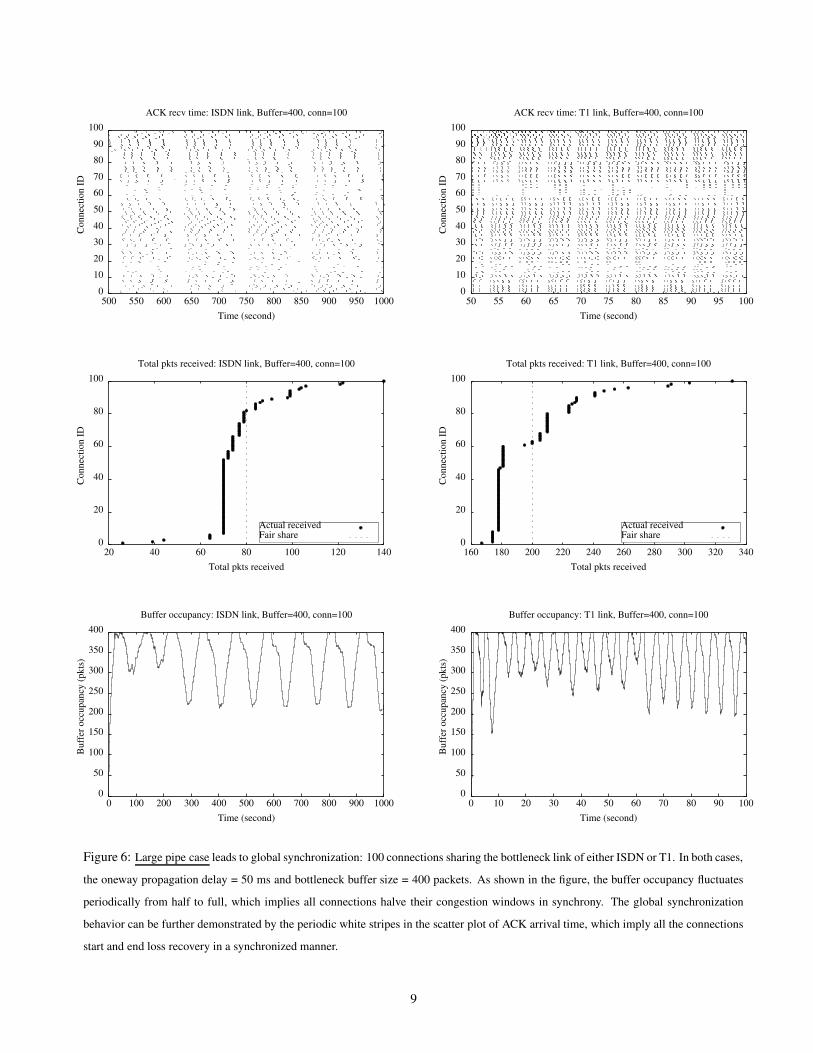
Figure 6 depicts the synchronization behavior. In all the graphs we sort the connection ID’s by the total number of

packets each connection has received, since such sorting reveals synchronization behavior more clearly. As shown in

the figure, the buffer occupancy periodically fluctuates from half to full, which implies all connections halve their congestion

windows in synchrony. The global synchronization behavior can be further demonstrated by the periodic white stripes in the

scatter plot of ACK arrival time, which imply all the connections start and end loss recovery in a synchronized manner.

The explanation for the synchronization behavior is similar to the case for small number of connections. Suppose at the

end of the current epoch the total number of outstanding packets from all the connections is equal to Wc. During the next

epoch all connections will increment their window. All the packets that are sent due to window increase will get dropped.

Thus all the connections will incur loss during the same RTT . This makes all connections adjust window in synchrony. When

Wc > 3 ∗ conn, most connections have more than 3 outstanding packets before the loss. So they can all recover the loss by

fast retransmissions, and reduce the window by half, leading to global synchronization. In contrast, when Wc < 3 ∗ Conn,

though all the connections still experience loss during the same RTT , they react to the loss differently. Some connections

whose cwnd is larger than 3 before the loss can recover the loss through fast recovery, whereas the others will have to use

timeout to recover the loss. Since the set of connections recovering loss using fast recovery and the set using timeout will

change over time, global synchronization cannot be achieved.

Due to global synchronization, all the connections share the resource very fairly: in the steady state they experience the

same number of losses and send the same number of packets. We can aggregate all the connections as one big connection,

and accurately predict the aggregate loss probability. All the original connections will have the same loss probability. More

specifically, if Wc is a multiple of Conn, let W = Wc

Connand b be the average number of packets acknowledged by an ACK.

During congestion avoidance phase, in each epoch other than the first and last ones, each connection’s window size starts

8

0

10

20

30

40

50

60

70

80

90

100

500 550 600 650 700 750 800 850 900 950 1000

Con

nect

ion

ID

Time (second)

ACK recv time: ISDN link, Buffer=400, conn=100

0

10

20

30

40

50

60

70

80

90

100

50 55 60 65 70 75 80 85 90 95 100

Con

nect

ion

ID

Time (second)

ACK recv time: T1 link, Buffer=400, conn=100

0

20

40

60

80

100

20 40 60 80 100 120 140

Con

nect

ion

ID

Total pkts received

Total pkts received: ISDN link, Buffer=400, conn=100

Actual receivedFair share

0

20

40

60

80

100

160 180 200 220 240 260 280 300 320 340

Con

nect

ion

ID

Total pkts received

Total pkts received: T1 link, Buffer=400, conn=100

Actual receivedFair share

0

50

100

150

200

250

300

350

400

0 100 200 300 400 500 600 700 800 900 1000

Buf

fer o

ccup

ancy

(pkt

s)

Time (second)

Buffer occupancy: ISDN link, Buffer=400, conn=100

0

50

100

150

200

250

300

350

400

0 10 20 30 40 50 60 70 80 90 100

Buf

fer o

ccup

ancy

(pkt

s)

Time (second)

Buffer occupancy: T1 link, Buffer=400, conn=100

Figure 6: Large pipe case leads to global synchronization: 100 connections sharing the bottleneck link of either ISDN or T1. In both cases,

the oneway propagation delay = 50 ms and bottleneck buffer size = 400 packets. As shown in the figure, the buffer occupancy fluctuates

periodically from half to full, which implies all connections halve their congestion windows in synchrony. The global synchronization

behavior can be further demonstrated by the periodic white stripes in the scatter plot of ACK arrival time, which imply all the connections

start and end loss recovery in a synchronized manner.

9

from bW+1

2c and increases linearly in time, with a slope of 1

bpacket per round trip time. When the window size reaches

W + 1, a loss occurs. Before the loss is detected by duplicated ACKs, another W packets are injected into the network. Then

the window drops back to bW+1

2c and a new epoch begins. Therefore, the total number of packets sent during an epoch can

be computed as S(T ) = b ∗ (∑W

x=bW+1

2c x) + 2 ∗ W + 1. Every connection incurs one loss during each epoch, so

Loss Probability =1

S(T )=

1

b ∗ (∑W

x=b W+1

2c x) + 2 ∗ W + 1

When b = 1,

Loss Probability =

8

3∗W 2+20∗W+9if W is odd

8

3∗W 2+22∗W+8otherwise

So we can approximate Loss Probability as

Loss Probability ≈8

3 ∗ W 2 + 21 ∗ W + 8.

Figure 7 shows our prediction matches very well to the actual loss probability.

0

0.01

0.02

0.03

0.04

0.05

0.06

1 10 100 1000

Los

s pr

obab

ility

Total connections

Loss probability: Buffer=4*Conn

actual losspredicted loss

0

0.005

0.01

0.015

0.02

0.025

0.03

0.035

0.04

0.045

1 10 100 1000

Los

s pr

obab

ility

Total connections

Loss probability: Buffer=6*Conn

actual losspredicted loss

Figure 7: Loss prediction for large pipe case: Varying number of connections sharing T1 link with one-way propagation delay of 50 ms,

and the bottleneck buffer is either 4 times or 6 times the number of connections.

Furthermore, as expected, global synchronization leads to periodical fluctuation in buffer occupancy as shown in Figure 6.

When the total buffer size is less than Wc

2, halving cwnd in synchrony leads to under-utilization of bottleneck link.

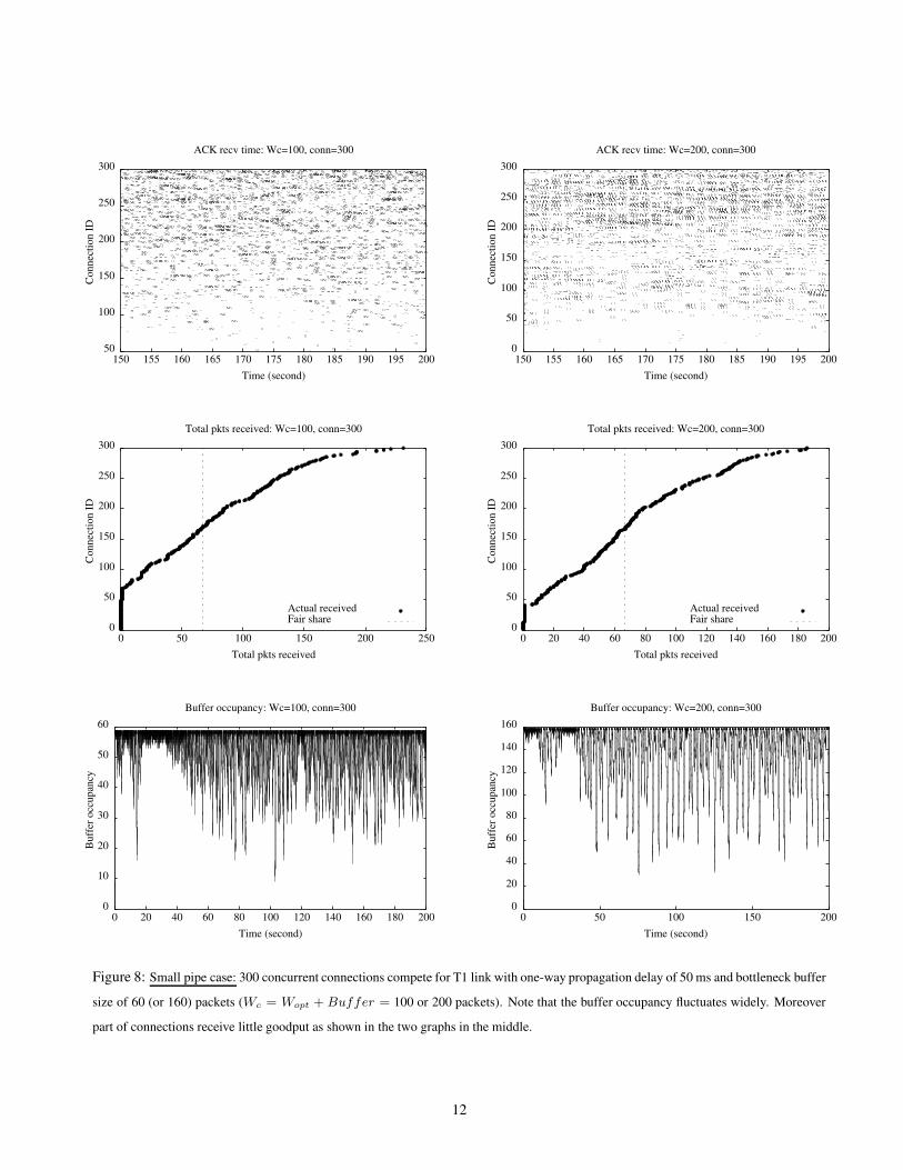
5.1.2 Case 2: Wc < Conn (Small pipe case)

When Wc < Conn, we have found TCP connections share the path very unfairly: only a subset of connections are active

(i.e. their goodput is considerably larger than 0), while the other connections are shut-off due to constant timeout as shown

in Figure 8. The number of active connections is close to Wc, and the exact value depends on both Wc and the number of

competing connections. When Conn exceeds the number of active connections the network resource can support, adding

more connections to the already overly congested network only adds more shut-off connections. Almost all the packets sent

from the shut-off connections get dropped. The remaining active connections are left mostly intact. This explains the curves

in Figure 9: when Conn is larger than the number of active connection the network resources can support, the total number

10

of packets sent and lost grows linearly with the number of connections. The linear increase in the number of packets sent and

lost mainly comes from the increase in the number of inactive (mostly shut-off) connections, each of which sends a constant

number of packets before it gets completely shut off.

5.1.3 Case 3: Conn < Wc < 3 ∗ Conn (Medium pipe case)

As shown in Figure 10, TCP behavior in this case falls in between the above two cases. More specifically, as explained earlier

(in Section 5.1.1), since 1 < Wc

Conn< 3, the connections respond to loss differently: some connections whose cwnd is larger

than 3 before the loss can recover the loss through fast recovery, whereas the others will have to use timeout to recover the

loss. Since the set of connections recovering loss using fast recovery and the set using timeout will change over time, no

global synchronization occurs, and the network resources are not shared as fairly as Wc > 3∗Conn. On the other hand, there

is still local synchronization, as shown Figure 10, where some groups of connections are synchronized within the groups.

Furthermore, since Wc

Conn> 1, all the connections can get reasonable amount of throughput. In contrast to the small pipe

case, there are almost no connections getting shut-off.

5.1.4 Aggregate Throughput

We define normalized aggregate TCP throughput as the number of bits sent by the bottleneck link in unit time normalized by

the link capacity. Our results are as follows:

• As shown in Figure 11(a), when the number of connections is small and the buffer size is less than Wopt (Wopt = 160

packets in this case), the normalized TCP throughput is less than 1. The degree of under-utilization depends on both the

number of connections and the ratio of the buffer size to Wopt. The smaller the number of connections and the lower

the ratio, the lower the network utilization is.

• As shown in Figure 11(b), when the buffer size is larger than Wopt (Wopt = 40 packets in this case), the normalized

TCP throughput is close to 1, regardless of the number of connections.

• When the number of connections is large, even if the buffer size is small (smaller than Wopt), the normalized TCP

throughput is close to 1. This is evident from Figure 11(a), where the throughput is close to 1 for large number of

connections under all the buffer sizes considered.

5.1.5 Aggregate Goodput

We define normalized aggregate goodput as the number of good bits received by all the receivers (excluding unnecessary

retransmissions) in unit time normalized by the link capacity. As shown in Figure 12,

• There is a linear decrease in goodput as the number of connections increases.

• The slope of the decrease depends on the bottleneck link bandwidth: the decrease is more rapid when the bottleneck

link is ISDN, and is slower when T1 is used as the bottleneck link.

These results can be explained as follows. The difference between the throughput and goodput is the number of unnecessary

retransmissions. As the number of connections increases, the loss probability increases, which in turn increases the number

of unnecessary retransmissions. Therefore the more connections, the lower the goodput is. On the other hand, since

loss in the normalized goodput =total unnecessary retransmissions

link capacity

11

50

100

150

200

250

300

150 155 160 165 170 175 180 185 190 195 200

Con

nect

ion

ID

Time (second)

ACK recv time: Wc=100, conn=300

0

50

100

150

200

250

300

150 155 160 165 170 175 180 185 190 195 200

Con

nect

ion

ID

Time (second)

ACK recv time: Wc=200, conn=300

0

50

100

150

200

250

300

0 50 100 150 200 250

Con

nect

ion

ID

Total pkts received

Total pkts received: Wc=100, conn=300

Actual receivedFair share

0

50

100

150

200

250

300

0 20 40 60 80 100 120 140 160 180 200

Con

nect

ion

ID

Total pkts received

Total pkts received: Wc=200, conn=300

Actual receivedFair share

0

10

20

30

40

50

60

0 20 40 60 80 100 120 140 160 180 200

Buf

fer o

ccup

ancy

Time (second)

Buffer occupancy: Wc=100, conn=300

0

20

40

60

80

100

120

140

160

0 50 100 150 200

Buf

fer o

ccup

ancy

Time (second)

Buffer occupancy: Wc=200, conn=300

Figure 8: Small pipe case: 300 concurrent connections compete for T1 link with one-way propagation delay of 50 ms and bottleneck buffer

size of 60 (or 160) packets (Wc = Wopt + Buffer = 100 or 200 packets). Note that the buffer occupancy fluctuates widely. Moreover

part of connections receive little goodput as shown in the two graphs in the middle.

12

38000

40000

42000

44000

46000

48000

50000

52000

54000

56000

0 100 200 300 400 500 600

Tot

al s

ent f

rom

sou

rces

Total connections

Total number of packets sent from sources: Wc=100

0

2000

4000

6000

8000

10000

12000

14000

16000

0 100 200 300 400 500 600

Tot

al lo

sses

Total connections

Total number of packets lost: Wc=100

Figure 9: Varying number of connections compete for T1 link with oneway propagation delay of 50 ms: the total number of packets sent

and dropped increases linearly with the number of connection when the connection number is large.

0

10

20

30

40

50

60

70

80

90

100

150 155 160 165 170 175 180 185 190 195 200

Con

nect

ion

ID

Time (second)

ACK recv time: Wc=200, conn=100, no overhead

0

20

40

60

80

100

0 50 100 150 200 250 300 350 400 450

Con

nect

ion

ID

Total pkts received

Total pkts received: Wc=200, conn=100, no overhead

Actual receivedFair share

0

20

40

60

80

100

120

140

160

0 50 100 150 200

Buf

fer o

ccup

ancy

Time (second)

Buffer occupancy: Wc=200, conn=100, no overhead

Figure 10: Medium pipe case: 100 concurrent connections compete for T1 link with one-way propagation delay of 50 ms and bottleneck

buffer size of 160 packets (Wc = Wopt +Buffer = 200 packets). Buffer occupancy fluctuates widely, and there is local synchronization

within some groups.

13

0.8

0.82

0.84

0.86

0.88

0.9

0.92

0.94

0.96

0.98

1

0 100 200 300 400 500 600

Nor

mal

ized

thro

ughp

ut

Total connections

Normalized throughput: T1 link with oneway propagation delay of 200 ms, varying buffer size

Buffer=10Buffer=20Buffer=40Buffer=60Buffer=110Buffer=160Buffer=200Buffer=300

0.965

0.97

0.975

0.98

0.985

0.99

0.995

1

0 100 200 300 400 500 600

Nor

mal

ized

thro

ughp

ut

Total connections

Normalized throughput: T1 link with oneway propagation delay of 50 ms, varying buffer size

Buffer=60Buffer=160Buffer=260Buffer=360Buffer=460

(a) (b)

Figure 11: Throughput: varying number of connections compete for the bottleneck link T1 with oneway propagation delay of either 200

ms or 50 ms

0.91

0.92

0.93

0.94

0.95

0.96

0.97

0.98

0.99

1

0 100 200 300 400 500 600

Nor

mal

ized

goo

dput

Total connections

Normalized goodput: ISDN link with oneway propagation delay of 50 ms, varying buffer size

Wc=100Wc=200Wc=300Wc=400Wc=500

0.96

0.965

0.97

0.975

0.98

0.985

0.99

0.995

0 100 200 300 400 500 600

Nor

mal

ized

goo

dput

Total connections

Normalized goodput: T1 link with oneway propagation delay of 50 ms, varying buffer size

Wc=100Wc=200Wc=300Wc=400Wc=500

Figure 12: Goodput: varying number of connections compete for the bottleneck link of either ISDN or T1. In both cases, the oneway

propagation delay=50 ms.

the decrease in the goodput is more substantial with slower bottleneck (e.g. ISDN), and less significant with faster bottleneck

(e.g. T1), which is evident from Figure 12.

To summarize, when the bottleneck link is fast or the loss probability is low (less than 20%), the number of unnecessary

retransmissions is negligible so that the normalized goodput is close to the normalized throughput. Otherwise (i.e. when the

bottleneck link is slow and the loss probability is high) the loss in the goodput due to unnecessary retransmissions becomes

significant. The decrease in the goodput depends on both the bottleneck link bandwidth and the loss probability.

5.1.6 Loss Probability

Our simulation results indicate when the Wc is fixed and the number of connections is small, the loss probability grows

quadratically with the increasing number of connections as shown in Figre 13. The quadratic growth in the loss probability

can be explained as follows. When Wc

Conn> 3, TCP connections can recover loss without timeouts. Every connection loses

14

one packet during each loss episode. So altogether there are Conn losses every episode. Meanwhile the frequency of loss

episode is proportional to Conn. Therefore for small number of connections, the loss probability is proportional to Conn2.

Such quadratic growth in loss probability is also reported in [10] for routers with RED dropping policy.

0.005

0.01

0.015

0.02

0.025

0.03

0.035

0.04

0 5 10 15 20 25 30 35 40 45 50

Los

s pr

obab

ility

Total connections

Loss probability: T1 link with oneway propagation delay of 50 ms, with buffer size=260 pkts

Wc=300

Figure 13: Loss probability for small number of connections: varying number of connections compete for the bottleneck link of T1 with

oneway propagation delay of 50 ms. The loss probability grows quadratically when the number of connections is small.

As the number of connections gets large (larger than Wc

3), the growth of loss probability with respect to the number of

connections matches impressively well with the following family of hyperbolic curves represented by

y =b ∗ x

x + a

as shown in Figure 14. Table 4 gives the parameters of the hyperbolic curves used in Figure 14. As part of our future work,

we will investigate how to predict the parameters of the hyperbolic curves given the network topology.

0

0.05

0.1

0.15

0.2

0.25

0.3

0.35

0.4

0 100 200 300 400 500 600

Los

s pr

obab

ility

Total connections

Loss probability: ISDN link with oneway propagation delay of 50 ms, varying buffer size

Wc=100Wc=200Wc=300Wc=400Wc=500

0

0.05

0.1

0.15

0.2

0.25

0.3

0 100 200 300 400 500 600

Los

s pr

obab

ility

Total connections

Loss probability: T1 link with oneway propagation delay of 50 ms, varying buffer size

Wc=100Wc=200Wc=300Wc=400Wc=500

Figure 14: Loss probability for large number of connections: varying number of connections compete for the bottleneck link of either

ISDN or T1. In both cases, the oneway propagation delay = 50 ms. The loss probability curves match very well with hyperbolic curves

when the number of connections is large, where the parameters of the hyperbolic curves are given in Table 4

15

ISDN T1

Wc a b Wc a b

100 149.2537 0.4646 100 144.9275 0.3237

200 333.3333 0.5262 200 285.7143 0.3429

300 588.2352 0.6059 300 454.5454 0.3682

400 1250.000 0.9170 400 526.3158 0.3517

500 2000.000 1.1852 500 769.2308 0.3948

Table 4: Parameters for the hyperbolic curves used for fitting loss probability as shown in Figure 14

5.2 TCP behavior with random overhead

5.2.1 Wc > 3 ∗ Conn (Large pipe case)

Our discussions in the previous section (Section 5.1) focus on the macro behavior of concurrent TCP connections with the

same propagation delay. In order to explore properties of networks with Drop Tail gateways unmasked by the specific details

of traffic phase effects or other deterministic behavior, we add random packet-processing time in the source nodes. This

is likely to be more realistic. The technique of adding random processing time was first introduced in [4]. However we

have different goals. In [4], Floyd and Jacobson are interested in how much randomness is necessary to break the systematic

discrimination against a particular connection. In contrast, we are interested in how much randomness is sufficient to break the

global synchronization. Consequently, the conclusions are different. [4] concludes that adding a random packet-processing

time ranging from zero to the bottleneck service time is sufficient; while we find that a random processing time that ranges

from zero to 10% ∗ RTT (usually much larger than a random packet service time) is required to break down the global

synchronization. This is shown in Figure 15, where the global synchronization is muted after adding the random processing

time up to 10% ∗ RTT .

The performance results in the non-synchronization case also differ from the global synchronization case. As shown in

Figure 16, when the number of connections is less than 100, the loss probability in the two cases are almost the same; as

the number of connections increases further, the gap between the two opens up: the non-synchronization case has higher

loss probability than the synchronization case. Nevertheless, using the prediction based on global synchronization gives a

reasonable approximation (at least a lower bound) of loss probability for non-synchronized case. However since in the non-

synchronization case, the connections do not share the bandwidth fairly. As shown in Figure 15, there is a large variation in

the throughput of different connections, so we can no longer predict the bandwidth share for each connection in this case.

A few comments follow:

• There is a general concern that synchronization is not good since it may lead to under-utilization of the bottleneck

bandwidth. However with the use of TCP-Reno and sufficient bottleneck buffer provisioning, this is unlikely to be a

problem in practice.

• There have been several attempts to break synchronization in order to avoid under-utilization. However our simulation

results indicate breaking down the synchronization using random processing time increases the unfairness and loss

probability.

16

0

10

20

30

40

50

60

70

80

90

100

500 550 600 650 700 750 800 850 900 950 1000

Con

nect

ion

ID

Time (second)

ACK recv time: ISDN link, Buffer=400, conn=100

0

10

20

30

40

50

60

70

80

90

100

50 55 60 65 70 75 80 85 90 95 100

Con

nect

ion

ID

Time (second)

ACK recv time: T1 link, Buffer=400, conn=100

0

20

40

60

80

100

0 50 100 150 200 250

Con

nect

ion

ID

Total pkts received

Total pkts received: ISDN link, Buffer=400, conn=100

Actual receivedFair share

0

20

40

60

80

100

50 100 150 200 250 300 350

Con

nect

ion

ID

Total pkts received

Total pkts received: T1 link, Buffer=400, conn=100

Actual receivedFair share

0

50

100

150

200

250

300

350

400

0 100 200 300 400 500 600 700 800 900 1000

Buf

fer o

ccup

ancy

(pkt

s)

Time (second)

Buffer occupancy: ISDN link, Buffer=400, conn=100

0

50

100

150

200

250

300

350

400

0 10 20 30 40 50 60 70 80 90 100

Buf

fer o

ccup

ancy

(pkt

s)

Time (second)

Buffer occupancy: T1 link, Buffer=400, conn=100

Figure 15: Adding random process time in large pipe case breaks down the global synchronization: 100 connections sharing the bottleneck

link of either ISDN or T1 with one-way propagation delay of 50 ms and bottleneck buffer size of 400 packets. Compared to the case of

without random processing time, the buffer occupancy is quite stable. Moreover global synchronization disappears as shown in the scatter

plot for ACK arrival.

17

0

0.01

0.02

0.03

0.04

0.05

0.06

0.07

0.08

0.09

0.1

0.11

1 10 100 1000

Los

s pr

obab

ility

Total connections

Loss probability

no overheadpredicted losswithin 1%*RTT overheadwithin 5%*RTT overheadwithin 10%*RTT overheadwithin 20%*RTT overheadwithin 50%*RTT overhead

Figure 16: Compare the loss probability by adding different amount of random processing time: varying number of connections compete

for T1 link with oneway propagation delay of 50 ms

5.2.2 Wc < Conn (Small pipe case)

Adding random processing time also affects the case when Wc < Conn. Without random processing time, we find there

is consistent discrimination against some connections, which end up totally shut off due to constant time-out. After adding

random processing time, there is still discrimination against some connections, but much less severe than before. As shown

in Figure 17, the number of shut-off connections is considerably smaller than before. Furthermore, the buffer occupancy is

mostly full and stable, whereas without random processing time, the buffer occupancy is quite low, and fluctuates a lot.

5.2.3 Conn < Wc < 3 ∗ Conn (Medium pipe case)

As shown in Figure 18, adding random processing time does not have much impact on TCP behavior in the case of medium

size pipe: as before, most connections get reasonable goodput, though not synchronized. On the other hand, the buffer

occupancy now becomes mostly full and stable in contrast to without random processing time, where the buffer occupancy is

low, and fluctuates a lot. In addition, even local synchronization disappears after adding random processing time.

5.2.4 Aggregate Throughput & Goodput

Adding random processing time has little effect in the overall throughput and goodput as shown in Figure 19 and Figure 20.

5.2.5 Loss Probability

For a small number of connections, adding random processing time makes the loss probability grow mostly linearly as the

number of connections increases. This is evident from Figure 21, which compares the loss probability curves before and after

adding random processing time.

For the large number of connections, adding random processing time does not change the general shape of the loss

probability curve: as before, the growth of loss probability with respect to the number of connections matches impressively

well with hyperbolic curves, as shown in Figure 22. On the other hand, for the same configuration (the same number of

connections and buffer size), the loss probability becomes larger after adding the random processing time. So the parameters

18

0

50

100

150

200

250

300

150 155 160 165 170 175 180 185 190 195 200

Con

nect

ion

ID

Time (second)

ACK recv time: Wc=100, conn=300

0

50

100

150

200

250

300

150 155 160 165 170 175 180 185 190 195 200

Con

nect

ion

ID

Time (second)

ACK recv time: Wc=200, conn=300

0

50

100

150

200

250

300

0 20 40 60 80 100 120 140 160

Con

nect

ion

ID

Total pkts received

Total pkts received: Wc=100, conn=300

Actual receivedFair share

0

50

100

150

200

250

300

0 20 40 60 80 100 120 140

Con

nect

ion

ID

Total pkts received

Total pkts received: Wc=200, conn=300

Actual receivedFair share

0

10

20

30

40

50

60

0 20 40 60 80 100 120 140 160 180 200

Buf

fer o

ccup

ancy

Time (second)

Buffer occupancy: Wc=100, conn=300

0

20

40

60

80

100

120

140

160

0 20 40 60 80 100 120 140 160 180 200

Buf

fer o

ccup

ancy

Time (second)

Buffer occupancy: Wc=200, conn=300

Figure 17: Adding random processing time in small pipe case: 300 concurrent connections compete for T1 link with one-way propagation

delay of 50 ms and buffer size of 60 (or 160) packets (Wc = Wopt + Buffer=100 or 200 packets). The buffer occupancy is quite stable,

and the consistent discrimination is not as severe as without adding random processing time.

19

0

10

20

30

40

50

60

70

80

90

100

150 155 160 165 170 175 180 185 190 195 200

Con

nect

ion

ID

Time (second)

ACK recv time: Wc=200, conn=100, up to 10% random overhead

0

20

40

60

80

100

50 100 150 200 250 300 350

Con

nect

ion

ID

Total pkts received

Total pkts received: Wc=200, conn=100, up to 10% random overhead

Actual receivedFair share

0

20

40

60

80

100

120

140

160

0 20 40 60 80 100 120 140 160 180 200

Buf

fer o

ccup

ancy

Time (second)

Buffer occupancy: Wc=200, conn=100,up to 10% random overhead

Figure 18: Adding random processing time in medium pipe case: 100 concurrent connections compete for T1 link with one-way propa-

gation delay of 50 ms and buffer size of 160 packets (Wc = Wopt + Buffer = 200 packets). The buffer occupancy is quite stable. In

contrast to without random processing time, there is no local synchronization.

0.84

0.86

0.88

0.9

0.92

0.94

0.96

0.98

1

0 100 200 300 400 500 600

Nor

mal

ized

thro

ughp

ut

Total connections

Normalized throughput: T1 link with oneway propagation delay of 200 ms, varying buffer size

Buffer=10Buffer=20Buffer=40Buffer=60Buffer=110Buffer=160Buffer=200Buffer=300

0.95

0.955

0.96

0.965

0.97

0.975

0.98

0.985

0.99

0.995

1

0 100 200 300 400 500 600

Nor

mal

ized

thro

ughp

ut

Total connections

Normalized throughput: T1 link with oneway propagation delay of 50 ms, varying buffer size

Buffer=60Buffer=160Buffer=260Buffer=360Buffer=460

Figure 19: Throughput after adding random processing time of up to 10% ∗RTT at TCP source: varying number of connections compete

for the bottleneck link of T1 link with propagation delay of either 200 ms or 50 ms

20

0.91

0.92

0.93

0.94

0.95

0.96

0.97

0.98

0.99

1

0 100 200 300 400 500 600

Nor

mal

ized

goo

dput

Total connections

Normalized goodput: ISDN link with oneway propagation delay of 50 ms, varying buffer size

Wc=100Wc=200Wc=300Wc=400Wc=500

0.86

0.88

0.9

0.92

0.94

0.96

0.98

1

0 100 200 300 400 500 600

Nor

mal

ized

goo

dput

Total connections

Normalized goodput: T1 link with oneway propagation delay of 50 ms, varying buffer size

Wc=100Wc=200Wc=300Wc=400Wc=500

Figure 20: Goodput after adding random processing time of up to 10% ∗ RTT at TCP source: varying number of connections compete

for the bottleneck link of either ISDN or T1. In both cases, the oneway propagation delay=50 ms.

0

0.01

0.02

0.03

0.04

0.05

0.06

0 2 4 6 8 10 12 14 16 18 20

Los

s pr

obab

ility

Total connections

Loss probability: T1 link with oneway propagation delay of 50 ms, buffer size=60

Wc=100, within10%*RTTWc=100, w/o overhead

0

0.005

0.01

0.015

0.02

0.025

0.03

0.035

0.04

0.045

0.05

0 5 10 15 20 25 30 35 40 45 50

Los

s pr

obab

ility

Total connections

Loss probability: T1 link with oneway propagation delay of 50 ms, with buffer size=260

Wc=300, within 10%*RTT overheadWc=300, w/o overhead

Figure 21: Loss probability for small number of connections after adding random processing time of up to 10% ∗ RTT at TCP source:

varying number of connections compete for the bottleneck link of T1 link with oneway propagation delay of 50 ms. The loss probability

grows linearly when the number of connections is small.

of hyperbolic curves are different as shown in Table 5.

5.3 TCP behavior with different RTT

It is well-known that TCP has bias against long roundtrip time connections. We are interested in quantifying this discrimina-

tion through simulations. Our simulation topology is similar to Figure 5 (in Section 4), except that we change the propagation

delay of the links. More specifically, we divide all the connections into two equal-size groups, where one group of connec-

tions has fixed propagation delay on the large bandwidth links, and the other group of connections has varying propagation

delay on the large bandwidth links. As suggested in [4], we add a random packet-processing time in the source nodes that

ranges from zero to the bottleneck service time to remove systematic discrimination. Our goal is to study how the throughput

ratio of two groups changes with respect to their RTT ’s.

Our simulation results are summarized in Figure 23, which plots the throughput ratio vs their RTT ratio both in log2

21

0

0.05

0.1

0.15

0.2

0.25

0.3

0.35

0.4

0.45

0 100 200 300 400 500 600

Los

s pr

obab

ility

Total connections

Loss probability: ISDN link with oneway propagation delay of 50 ms, varying buffer size

Wc=100Wc=200Wc=300Wc=400Wc=500

0

0.05

0.1

0.15

0.2

0.25

0.3

0.35

0.4

0 100 200 300 400 500 600

Los

s pr

obab

ility

Total connections

Loss probability: T1 link with oneway propagation delay of 50 ms, varying buffer size

Wc=100Wc=200Wc=300Wc=400Wc=500

Figure 22: Loss probability for large number of connections after adding up to 10%∗RTT at TCP source: varying number of connections

compete for the bottleneck link of either ISDN or T1. In both cases, the oneway propagation delay = 50 ms. The loss probability curves

match very well with hyperbolic curves when the number of connections is large, where the parameters of the hyperbolic curves are given

in Table 5

ISDN T1

Wc k Scale Wc k Scale

100 125.0000 0.4930 100 125.0000 0.4263

200 217.3913 0.5257 200 227.2727 0.4505

300 400.0000 0.6071 300 333.3333 0.4690

400 714.2857 0.7536 400 500.0000 0.5123

500 1428.5714 1.1110 500 666.6666 0.5366

Table 5: Parameters for the hyperbolic curves used for fitting loss probability as shown in Figure 22

scale. As shown in Figure 23, the throughput ratio is bounded by two curves. More specifically, when RTT1 ≤ RTT2,

(RTT2

RTT1

)2 ≤Throughput1

Throughput2≤ 2 ∗ (

RTT2

RTT1

)2 A(1)

where RTT1 and RTT2 are the average RTT the connections in group 1 and group 2 experience respectively. Since we can

swap the labels for groups 1 and 2, so the throughput ratio is symmetric as shown in Figure 23(a).

Now let’s try to explain the relationship (A1). For ease of discussion, we aggregate all the connections in one group as a

big connection. So in the following we just consider two connections compete with each other. Moreover, due to symmetry,

we only need to consider the case when RTT1 ≤ RTT2.

Figure 24 depicts roughly how the congestion windows evolve during congestion for two connections with different RTT.

As shown in the figure, during every epoch the cwnd of connection i grows from Wi to Wi ∗ 2. So the average length of

epoch, denoted as Ei, is roughly equal to RTT ∗ Wi. Therefore

Throughputi =3 ∗ W 2

i

2∗

1

Ei=

3 ∗ Wi

2 ∗ RTTi

(A2)

.

22

0.0625

0.125

0.25

0.5

1

2

4

8

16

0.5 1 2

Thr

ough

put2

/Thr

ough

put1

RTT1/RTT2

Throughput ratio under different RTT with 40 conns (each group with 20 conns)

Actual ratio2*(RTT1/RTT2)^2(RTT1/RTT2)^2/2(RTT1/RTT2)^2

0.5

1

2

4

8

16

1 2 4

Thr

ough

put2

/Thr

ough

put1

RTT1/RTT2

Throughput ratio under different RTT with 20 conns (each group with 10 conns)

Actual ratio(RTT1/RTT2)^2/2(RTT1/RTT2)^2

(a) (b)

Figure 23: Two groups of TCP connections compete for T1 link with oneway propagation delay of 50 ms

Now let x denote E1

E2. Using (A2), we have

Throughput1

Throughput2= (

RTT2

RTT1

)2 ∗ x.

Applying the equality of A(1), we obtain 1 ≤ x ≤ 2. This means the average epoch length of connection 1 is usually no

larger than twice the epoch length of connection 2. That is, for every two losses in connection 2, on average there is usually

at least one loss in connection 1. This implies there is no consistent discrimination against any particular connection, which

is likely to be the case after adding random processing time [4].

Time

cwnd

W2

W1

Figure 24: Window evolution graph for two connections with different RTT’s

The roundtrip time bias in TCP/IP networks has received lots of attention. There have been a number of studies on

analyzing such bias. [8] gives analytical explanation for this, and concludes the ratio of the throughput of two connections

(i.e. Throughputi

Throughputj) is proportional to (

RTTj

RTTi)2. The analysis is based on TCP-Tahoe window evolution. As pointed out in [8],

since in TCP-Reno the number of times the window is halved at the onset of congestion equals the number of lost packets, and

since phase effects can cause one connection to systematically lose a large number of packets, it is possible that a connection

gets almost completely shut off. Therefore the throughput ratio of two connections using TCP-Reno is unpredictable: the

connection with smaller propagation delay can sometimes get lower throughput due to systematical discrimination. Our

simulation study shows that though the throughput ratio of two connections may fluctuate a lot, the aggregate throughput

ratio of two groups of connections is relatively stable when the group size is reasonably large. Furthermore, the analysis

in [8] is based on the assumption that two connections with different RTT’s are synchronized. This does not always hold.

23

Therefore the throughput ratios Throughput2Throughput1

do not match very well with the curve ( RTT1

RTT2)2 as shown in Figure 23. Instead

our results indicate the throughput ratio is clustered within a band close to ( RTT1

RTT2)2, and the width of the band is usually one

unit in log2 scale.

As part of our future work, we will investigate how TCP behaves when the number of different RTT groups increases.

Also we are interested in examining how the performance is affected when the number of connections in each group is

unequal.

6 Related Work

Large scale performance analysis has been an active research area recently. Many researches are currently focused on building

scalable simulators, such as [1, 6, 16].

Analyzing simulation results to estimate TCP performance, as done in this project, is a very different approach from

building a scalable simulator. The strategy taken by [10] is the closest to ours. It studies how TCP throughput, loss rates,

and fairness are affected by changing the number of flows. Their work differs from ours in that we have created a generic

abstract model of Internet connection, and focused on studying how TCP performance changes by varying parameters of the

model, whereas they focus on studying how the TCP behaves as one of the parameters - the number of flows changes, while

keeping all the other parameters to be something reasonable. Furthermore they study TCP tahoe assuming RED dropping

policy at the routers, whereas we study TCP reno using drop-tail, since they are more widely deployed in today’s Internet.

RED dropping policy is not sensitive to instantaneous queue occupancy, so it is relatively easy to obtain the steady state

performance. A number of analytical models have been developed for studying the steady state TCP throughput when routers

use RED dropping policy [9, 17]. However modeling multiple connections sharing a bottleneck link with drop-tail policy is

much more challenging, since such policy is very sensitive to the instantaneous queue occupancy, and loss is non-randomized.

Simulation approach, as employed in this paper, proves to be an effective approach for studying TCP performance under drop

tail policy.

7 Conclusion and Future Work

In this paper, we have investigated the individual and aggregate TCP performance. We first develop a generic network

model that captures the essence of wide area Internet connections. Based on the abstract model, we study the behavior of a

single TCP connection under other competing TCP flows by evaluating the TCP analytical model proposed in [13]. We also

examine the aggregate behavior of many concurrent TCP flows. Through extensive simulations, we have identified how TCP

performance is affected with changing parameters in the network model. These results give us valuable insights into how

TCP behaves in diverse Internet.

There are a number of directions for future work. First, we have shown the loss probability curves can be approximated

quite well with simple analytical functions. As part of our future work, we will investigate how to quantitatively determine

the parameters in the functions. Second, we plan to further explore TCP performance under different RTT’s. In particular,

we want to consider the following two extensions: (i) when the two different RTT groups are not equal size; and (ii) with

different number of RTT groups. Finally, we plan to use Internet experiments to verify some of the results in the paper.

24

References

[1] J. Ahn and P. B. Danzig. Speedup vs. Simulation Granularity. [unpublished]

[2] N. Cardwell, S. Savage, and T. Anderson. Modeling the Performance of Short TCP Connections. Techical Report.

[3] S. Floyd. Connections with Multiple Congested Gateways in Packet-Switched Networks Part 1: One-way Traffic. Com-

puter Communication Review, Vol.21, No.5, October 1991, p. 30-47.

[4] S. Floyd and V. Jacobson. On Traffic Phase Effects in Packet-Switched Gateways. Internetworking: Research and Expe-

rience, V.3 N.3, September 1992, p.115-156.

[5] S. Floyd and V. Jacobson. Random Early Detection Gateways for Congestion Avoidance. IEEE/ACM Transactions on

Networking, V.1 N.4, August 1993, p. 397-413.

[6] P. Huang, D. Estrin, and J. Heidemann. Enabling Large-scale Simulations: Selective Abstraction Approach to the Study

of Multicast Protocols. USC-CS Technical Report 98-667, January 1998.

[7] S. Keshav. An Engineering Approach to Computer Networking, Addison-Wesley, 1997.

[8] T. V. Lakshman and U. Madhow. Performance Analysis of Window-based Flow Control using TCP/IP: Effect of High

Bandwidth-Delay Products and Random Loss. In Proc. IFIP TC6/WG6.4 Fifth International Conference on High Perfor-

mance Networking, June 1994.

[9] M. Mathis, J. Semke, J. Mahdavi, and T. Ott. Macroscopic Behavior of the TCP Congestion Avoidance Algorithm.

Computer Communication Review, July 1997.

[10] R. Morris. TCP Behavior with Many Flows. In Proc. IEEE International Conference on Network Protocols ’97, October

1997.

[11] UCB/LBNLVINT Network Simulator - ns (version 2). http://www-mash.cs.berkeley.edu/ns, 1997.

[12] V. Paxson. Automated Packet Trace Analysis of TCP Implementations. In ACM SIGCOMM’97, 1997.

[13] J. Padhye, V. Firoiu, D. Towsley, and J. Kurose, Modeling TCP Throughput: A Simple Model and Its Empirical Valida-

tion. In Proc. ACM SIGCOMM ’98, 1998.

[14] S. Keshav. REAL 5.0 Overview. http://www.cs.cornell.edu/skeshav/real/overview.html

[15] S. Shenker, L. Zhang, and D. D. Clark. Some Observations on the Dynamics of a Congestion Control Algorithm. ACM

Computer Communication Review pp.30-39, 1990.

[16] VINT. http://netweb.usc.edu/vint.

[17] X. Yang. A Model for Window Based Flow Control in Packet-Switched Networks. In IEEE INFOCOM ’99, 1999.

[18] E. W. Zegura, K. L. Calvert, and M. J. Donahoo. A Quantitative Comparison of Graph-Based Models for Internet

Topology. IEEE/ACM Transactions on Networking, December 1997.

25