On Joint Modelling and Testing for Localand Global Spatial Externalities 1

Zhenlin Yang

School of Economics and Social Sciences, Singapore Management University,

90 Stamford Road, Singapore 178903. zlyang@smu.edu.sg

October 2006

Abstract

This paper concerns the joint modeling, estimation and testing for local and

global spatial externalities. Spatial externalities have become in recent years a

standard notion of economic research activities in relation to social interactions,

spatial spillovers and dependence, etc., and have received an increasing attention

by econometricians and applied researchers. While conceptually the principle un-

derlying the spatial dependence is straightforward, the precise way in which this

dependence should be included in a regression model is complex. Following the

taxonomy of Anselin (2003, International Regional Science Review 26, 153-166),

a general model is proposed, which takes into account jointly local and global ex-

ternalities in both modelled and unmodelled effects. The proposed model encom-

passes all the models discussed in Anselin (2003). Robust methods of estimation

and testing are developed based on Gaussian quasi-likelihood. Large and small

sample properties of the proposed methods are investigated.

Key words and phrases: Asymptotic property, Finite sample property, Quasi-likelihood,

Spatial regression models, Robustness, Tests of spatial externalities.

JEL Classification: C1, C2, C5

1The author thanks Ingmar R. Prucha, Rossi Cristina, Liangjun Su and the participants at the

International Workshop on Spatial Econometrics and Statistics (Rome, Italy, 25-27 May 2006) for

helpful comments. Support from a research grant (Grant number: C208/MSS5E013) from Singapore

Management University is gratefully acknowledged.

1 Introduction

Spatial dependence or social interaction among the economic or social actors has

recently received a greatly increased attention (Anselin 2003; Goodchild et al. 2000;

Glaeser et al. 1996; Akerlof 1997; Abbot 1997; Sampson et al. 1999). Spatial economet-

ric models and methods have been applied not only in specialized fields such as regional

science, urban economics, real estate and economic geography, but also increasingly

in more traditional fields of economics as well, including demand analysis, labor eco-

nomics, public economics, international economics, and agricultural and environmental

economics (see reviews in Anselin and Bera 1998; Anselin 2001; and Elhorst 2003).

While conceptually it is straightforward to see the principle underlying the resulting

spatial dependence, the precise way in which this dependence should be included in

a regression model is rather complex. Very recently, the notions of local and global

externalities or short range and long range spatial dependence were brought up by

Anselin (2003), which since then has caught the attention of many econometricians and

applied researchers. Anselin provided a comprehensive taxonomy of spatial econometric

models according to different kinds of spatial externalities in an effort to better reconcile

econometric practice with theoretical developments. However, the problems of model

estimation and testing for some models are not considered; joint modeling and testing

of local and global spatial externalities is not discussed; and consistency and asymptotic

normality of the parameter estimates for certain models are not formally treated. Thus,

it is highly desirable to“unify” all the available models and develop general methods of

inference, allowing flexible spatial patterns in the model so that an appropriate one can

be identified by the data through testing.

In this article, I propose a general model that takes into account of local and global

externalities jointly, in both modelled effects as well as unmodelled effects. The proposed

model contains the models discussed in Anselin (2003) and other models available in

the literature as special cases. I propose using the quasi-maximum likelihood method

(QMLE) for model estimation. QMLE is advantageous over the traditional maximum

likelihood estimation (MLE) method in that it is robust against misspecification in error

2

distribution, and is advantageous over the IV or GMM in that it is applicable to a pure

spatial process (a model of no covariates), see Lee (2004a). The problem of parameter

identifiability, and the consistency and asymptotic normality of the QMLE are formally

treated, to set foundations for formal statistical inferences. Tests (joint or marginal)

for local and global externalities are developed to facilitate the practitioners to choose

the model. These tests all possess simple analytical expressions, and are robust against

nonnormality of the error distributions. Monte Carlo simulation shows that both the

QMLEs and the tests perform very well in finite samples.

The rest of the paper is organized as follows. Section 2 presents the general model

and the quasi-maximum likelihood estimation (QMLE) procedure. Section 3 treats the

problems of parameter identifiability, and the consistency and asymptotic normality of

the QMLE. Section 4 presents various tests for spatial externalities. Section 5 presents

Monte Carlo results for finite sample performance of the proposed methods. Section 6

concludes the paper.

2 A General Spatial Regression Model

In this section, I present a general spatial regression model that takes into account

of local and global externalities in the modelled effects as well as the local and global

externalities in the unmodelled effects, focusing more on the practical issues of model

estimation and covariance estimation to facilitate the practical applications.

2.1 The model

For an n× n spatial contiguity weights matrix Wn, multiplication of In + ρWn on a

variable generates a local spatial externality, and multiplication of (In − ρWn)−1 on a

variable generates a global spatial externality, where In is an n× n identity matrix andρ is a spatial parameter. See Anselin (2003, Sec. 2) for detailed explanations. A natural

generalization of these ideas is to multiply (In + ρ1Wn)(In − ρ2Wgn)−1 on a variable

to generate simultaneously local and global spatial externalities, where Wn and Wgn

3

are, respectively, the local and global spatial weights matrices. Loosely speaking, local

spatial externality means that spatial dependence is limited to among the “neighbors”,

whereas the global spatial externalities means that the spatial dependence exists among

the spatial units that may be “far” away from each other. Spatial externalities may

exist in the modeled effects (the regressors) as well as in the unmodelled effects (the

errors). To give a maximum generality, I consider both local and global externalities

in both modelled as well as unmodeled effects.2 Generically, let A(W1n,Wg1n, ρ) be an

n× n matrix function of the n× n spatial weights matrices W1n and Wg1n, indexed by a

k1 × 1 spatial parameter vector ρ, and B(W2n,Wg2n, γ) be an n × n matrix function of

the n× n spatial weights matrices W2n and Wg2n, indexed by a k2 × 1 spatial parameter

vector γ. The proposed model takes the following general form:

Yn = A(W1n,Wg1n, ρ)Xnβ +B(W2n,W

g2n, γ)un (1)

where the matrices A(W1n,Wg1n, ρ) ≡ An(ρ) and B(W2n,W

g2n, γ) ≡ Bn(γ) capture, re-

spectively, the spatial externalities in the covariates Xn and in the error vector un, β is

a p × 1 vector of model parameters, and un is a vector of independent and identicallydistributed (iid) errors of mean zero and variance σ2. All W matrices are normalized to

have unity row sums. Clearly, it must be that An(0) = In and Bn(0) = In, i.e., ρ = 0 or

γ = 0 or both indicates the lack of spatial externality in Xn or in un or in both.

The model given in (1) is very general, covering most of the models available in

the literature. From the above discussions, we see that the local spatial externality

corresponds to a spatial moving average (SMA) process, the global spatial externality

corresponds to a spatial autoregressive (SAR) process, and the local and global spatial

externalities together correspond to a spatial autoregressive moving average (SARMA)

process.3 Most of the models appeared in the literature apply one or more of the these

2Spatial effects in Yn can be converted to the spatial effects in Xn and error terms, see Anselin(2003).3This term is originated from Huang (1984), with the original meaning being a SAR(p) for the

response together with a SMA(q) for the error. However, we see no reason why we can not apply a

SAR(p) and a SMA(q) to the same variable to produce a SARMA(p, q) error, or a SARMA(p, q) re-

sponse, or SARMA(p, q) regressors. See also Bera and Anselin (1998) and Anselin (2003) for discussions

on SARMA processes.

4

processes (first order or higher)4 to one or more of the model components: the response,

the regressors, and the disturbance. These can all be reduced to the form specified in

Model (1) defined above, with certain constrains (when necessary) being put on ρ and

γ, and on the weights matrices. For example, in their popular forms, we have,

• Yn = Xnβ+εn, with εn = γWnεn+un. This is a model with a SAR(1) error or global externality

on un, which can be written in the form of (1) with An(ρ) = In and Bn(γ) = (In−γWn)−1 (see,

e.g., Anselin and Bera, 1998; Benirschka and Binkley, 1994; Kelejian and Prucha, 1999);

• Yn = Xnβ+εn, with εn = γWnun+un, a model with a SMA(1) error or local externality on un.

In the form of (1), An(ρ) = In and Bn(γ) = (In + γWn) (see, e.g., Cliff and Ord 1981; Haining

1990; Anselin and Bera 1998).

• Yn = ρWnYn+Xnβ+un, a model with only a SAR(1) on Yn, which can be translated into a model

with global externality in both Xn and un, with An(ρ) = (In− ρWn)−1, Bn(γ) = (In− γWn)

−1,

and ρ = γ (see, e.g., Anselin 1988; Case et al. 1993; Besley and Case 1995; Lee 2002, 2004a);

• Yn = Xnβ + ρW1nXnβ + εn with εn = γWnεn + un. This is a model with a SMA(1) on Xn and

a SAR(1) on un, called the hybrid model by Anselin (2003). For this model, An(ρ) = In + ρWn

and Bn(γ) = (In−γWn)−1. It has not been formally studied so far. Alternatively, one can apply

SAR(1) on Xn and SMA(1) on un;

• Yn = ρW1nYn + Xnβ + εn with εn = γW2nεn + un, a model with SAR(1) on both Yn and εn

(see Anselin 1988, p. 60-65). It has been applied by, among others, Case (1991, 1992), Case et

al. (1993), and Besley and Case (1995). It is called the spatial ARAR(1,1) model by Kelejian

and Prucha (1998, 2001, 2006), who studied generalized spatial 2SLS procedure, asymptotic

distribution of Moran I test, and GM estimation of the model with heteroscedastic errors. Using

our notation, we have An(ρ) = (In − ρW1n)−1 and Bn(γ) = (In − γ1W

g2n)−1(In − γ2W2n)

−1,

with γ1 = ρ, γ2 = γ, W g2n =W1n, and W2n =W2n.

• Yn = Xnβ+εn with εn = γ1Wgnεn+γ2Wnun+un, a model with SARMA(1,1) (or joint local and

global spatial externalities) on errors. In this case, An(ρ) = In and Bn(γ) = (In−γ1W gn)−1(In+

γ2Wn);

• Yn = Znβ + εn, with Zn = ρ1Wg1nZn + ρ2WnXn + Xn, and εn = γ1W

g2nεn + γ2W2nun + un,

a model with a SARMA(1,1) on un and a SARMA(1,1) on Xn. In this case, An(ρ) = (In −ρ1W

g1n)−1(In + ρ2W1n) and Bn(γ) = (In − γ1W g

2n)−1(In + γ2W2n).

4Higher-order spatial lag operators are defined by applying the spatial weights matrix to a lower-

order lagged variable, e.g., a second-order spatial lag in Yn is obtained asWn(WnYn) =W2nYn. However,

higher-order spatial operators yield redundant and circular neighbor relations, which must be eliminated

to ensure proper estimation and inference (Anselin and Bera, 1998, p. 247).

5

Clearly, the model can be more complicated than any of them listed above. For

example, one may use (In+ γ1Wn + γ2W2n + γ3W

3n) to generate local effects that extend

to several layers of neighbors. Also, the general specification given in (1) can be easily

extended to include covariates that are not associated with any spatial effects, and to

add heteroscedasticity structure onto the model.

2.2 Model estimation

I now outline the quasi-maximum likelihood estimation (QMLE) procedure based on

Gaussian likelihood. Let Ωn(γ) = Bn(γ)Bn(γ). Let θ = (ρ , γ ) , and ξ = (β , θ ,σ2) .

The quasi-loglikelihood, using normal distribution as an approximation to the error

distribution, has the form

n(ξ) = −n2ln(2πσ2)− 1

2ln |Ωn(γ)|− 1

2σ2εn(β, ρ) Ω

−1n (γ)εn(β, ρ) (2)

where εn(β, ρ) = Yn −An(ρ)Xnβ. Given θ, the constrained QMLEs of β0 and σ20 are

βn(θ) = [Xn(ρ) Ω−1n (γ)Xn(ρ)]

−1Xn(ρ)Ω−1n (γ)Yn (3)

σ2n(θ) =1

n[Yn −Xn(ρ)βn(θ)] Ω−1n (γ)[Yn −Xn(ρ)βn(θ)], (4)

where Xn(ρ) = An(ρ)Xn.

Substituting βn(θ) and σ2n(θ) back into (2) for β and σ

2, we obtain the concentrated

quasi-loglikelihood function for θ.

cn(θ) = −

n

2[1 + ln(2π)]− 1

2ln |Ωn(γ)|− n

2ln[σ2n(θ)]. (5)

Maximizing cn(θ) gives the QMLE θn of θ, which in turn gives the QMLEs of β and σ

2

as βn = βn(θn) and σ2n = σ2n(θn). Maximization ofcn(θ) can be conveniently realized

using GAUSS CO procedure (see the footnote to Assumption I in Section 3 for the issue

of parameter space). In cases where computing speed is an issue, one may consider

providing the analytical gradient

∂ cn(θ)

∂ρi=

[Xn,ρi(ρ)βn(θ)] Ω−1n (γ)εn(βn(θ), ρ)

εn(βn(θ), ρ)Ω−1n (γ)εn(βn(θ), ρ)/n

, (6)

∂ cn(θ)

∂γj=

εn(βn(θ), ρ)Ω−1n (γ)Ωn,γj(γ)Ω

−1n (γ)εn(βn(θ), ρ)

2εn(βn(θ), ρ)Ω−1n (γ)εn(βn(θ), ρ)/n

− 12tr[Ω−1n (γ)Ωn,γj(γ)], (7)

6

where i = 1, · · · , k1, j = 1, · · · , k2, Xn,ρi(ρ) = ∂∂ρiXn(ρ) and Ωn,γj(γ) =

∂∂γjΩn(γ). For

large data, repeated calculation of |Ωn(γ)| as required in the process of maximizingcn(θ) can be a burden. However, often the special form of the Ωn(γ) matrix allows

for a considerable amount of simplifications. For example, in a model with a spatial

AR error, Bn(γ) = (In − γW2n)−1. Thus Ωn(γ) = [(In − γW2n)(In − γW2n)]

−1 and

|Ωn(γ)| = ni=1(1 − γwi)

−2, where wi are the eigenvalues of W2n. As W2n is a fixed

matrix, its eigenvalues only need to be calculated once and be used subsequently.5

2.3 Covariance estimation

The previous subsection describes a simple procedure for model estimation. Formal

statistical analysis needs the standard errors of the parameter estimates, or more gener-

ally the variance-covariance estimate of the QMLE to facilitate more advanced statistical

inferences such as confidence interval construction for quantiles. To provide a simple ex-

pression for such a covariance estimate, some notation and conventions are necessary,

and these notation and conventions will be followed through the rest of the article.

Notation and conventions. Let ξ0 (and accordingly β0, θ0, ρ0, γ0 and σ20) represent

the true parameter values. Let Gn(ξ) =∂∂ξ n(ξ) be the gradient vector and Hn(ξ) =

∂∂ξGn(ξ) be the Hessian matrix with their detailed expressions given in Appendix A.

Let Kn(ξ0) = Var[Gn(ξ0)] and In(ξ0) = −E[Hn(ξ0)], with the expectation and varianceoperators ‘E’ and ‘Var’ corresponding to the true parameters. Specifically, E(Yn) =

An(ρ0)Xnβ0 and Var(Yn) = σ20Ω(γ0). For a vector vn and a matrix Mn, vn,i is the ith

element of vn, mn,ij is the ijth element ofMn, vn is the Euclidean norm of vn, tr(Mn)

is the trace of Mn, diagv(Mn) is a column vector formed by the diagonal elements of

Mn, |Mn| is the determinant, Mn is the transpose, and M−1n is the inverse of Mn. The

partial derivatives of the matrix function An(ρ) with respect to the ith element of ρ is

denoted as An,ρi(ρ). Similar notation is used for the partial derivatives of Bn(γ), Xn(ρ)

5Accuracy issue may arise when n is large (Kelejian and Prucha, 1998), and in this case sparce

matrix technique should be employed (LeSage, 1999). See Griffith, 1988; Anselin, 1988; Magnus, 1982;

and Magnus and Neudecker, 1999, for more on matrix calculations.

7

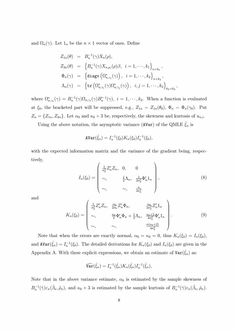
and Ωn(γ). Let 1n be the n× 1 vector of ones. Define

Z1n(θ) = B−1n (γ)Xn(ρ),

Z2n(θ) = B−1n (γ)Xn,ρi(ρ)β, i = 1, · · · , k1 n×k1,

Φn(γ) = diagv Ω∗n,γi(γ) , i = 1, · · · , k2 n×k2,

Λn(γ) = tr Ω∗n,γi(γ)Ω∗n,γj(γ) , i, j = 1, · · · , k2

k2×k2,

where Ω∗n,γi(γ) = B−1n (γ)Ωn,γi(γ)B−1n (γ), i = 1, · · · , k2. When a function is evaluated

at ξ0, the bracketed part will be suppressed, e.g., Z1n = Z1n(θ0), Φn = Φn(γ0). Put

Zn = Z1n, Z2n. Let α0 and κ0 + 3 be, respectively, the skewness and kurtosis of un,i.Using the above notation, the asymptotic variance (AVar) of the QMLE ξn is

AVar(ξn) = I−1n (ξ0)Kn(ξ0)I

−1n (ξ0),

with the expected information matrix and the variance of the gradient being, respec-

tively,

In(ξ0) =

⎛⎜⎜⎜⎜⎜⎜⎜⎝

1σ20ZnZn, 0, 0

∼, 12Λn,

12σ20Φn1n

∼, ∼, n2σ40

⎞⎟⎟⎟⎟⎟⎟⎟⎠ , (8)

and

Kn(ξ0) =

⎛⎜⎜⎜⎜⎜⎜⎜⎝

1σ20ZnZn,

α02σ0ZnΦn,

α02σ30Zn1n

∼, κ04ΦnΦn +

12Λn,

κ0+24σ20

Φn1n

∼, ∼, n(κ0+2)4σ40

⎞⎟⎟⎟⎟⎟⎟⎟⎠ . (9)

Note that when the errors are exactly normal, α0 = κ0 = 0, thus Kn(ξ0) = In(ξ0),

and AVar(ξn) = I−1n (ξ0). The detailed derivations for Kn(ξ0) and In(ξ0) are given in the

Appendix A. With these explicit expressions, we obtain an estimate of Var(ξn) as:

Var(ξn) = I−1n (ξn)Kn(ξn)I

−1n (ξn),

Note that in the above variance estimate, α0 is estimated by the sample skewness of

B−1n (γ)εn(βn, ρn), and κ0 + 3 is estimated by the sample kurtosis of B−1n (γ)εn(βn, ρn).

8

Clearly, use of QMLE standard error makes the inferences robust against the excess

skewness and kurtosis of the data. When the focus of statistical inference is on the

regular regression parameters β as is the case for the empirical applications, a simple

inferential statistic is presented in Section 4.

3 Large Sample Properties

In this section, I consider the problems of parameter identifiability, and consistency

and asymptotic normality of the QMLEs. These asymptotic theories are essential for

statistical inferences for the regression coefficients, and for testing the local and global

spatial effects. Let Θ1 be the parameter space containing the values of ρ, Θ2 be the

space of γ values, and Θ = Θ1 × Θ2 be the product space containing the values of

θ. The following is a set of regularity conditions that are sufficient for the parameter

identifiability and consistency of the QMLEs.

Assumption 1. The space Θ is compact with θ0 being an interior point of it.6

Assumption 2. un,i are iid with mean zero, variance σ20, and finite moment

E(|un,i|4+ ) for > 0.

Assumption 3. The elements of Xn are uniformly bounded, and limn→∞ 1n[Z1n(θ)Z1n(θ)]

exists and is nonsingular, uniformly in θ ∈ Θ.Assumption 4. The sequences of matrices An(ρ) and A

−1n (ρ) are uniformly bounded

in both absolute row or column sums, uniformly in ρ ∈ Θ1.Assumption 5. The sequences of matrices Bn(γ) and B

−1n (γ) are uniformly bounded

in both absolute row and column sums, uniformly in γ ∈ Θ2,Assumption 6. Z1n(θ) and Z2n(θ) are not asymptotically multicolinear, uniformly

in θ ∈ Θ; and limn→∞ 1n[Z2n(θ)Z2n(θ)] exists and is nonsingular, uniformly in θ ∈ Θ.

6Kelejian and Prucha (2006) address an important issue on parameter space when spatial weights

matrices are not row-normalized, leading to a practical definition of the parameter space that is typically

n-dependent.

9

Assumption 7. The elements of An,ρi(ρ), i = 1, · · · , k1, are uniformly bounded,uniformly in ρ ∈ Θ1; and the elements of Bn,γj(γ), j = 1, · · · , k2, are uniformly bounded,uniformly in γ ∈ Θ2.

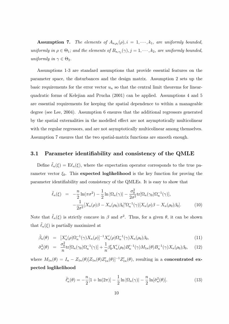
Assumptions 1-3 are standard assumptions that provide essential features on the

parameter space, the disturbances and the design matrix. Assumption 2 sets up the

basic requirements for the error vector un so that the central limit theorems for linear-

quadratic forms of Kelejian and Prucha (2001) can be applied. Assumptions 4 and 5

are essential requirements for keeping the spatial dependence to within a manageable

degree (see Lee, 2004). Assumption 6 ensures that the additional regressors generated

by the spatial externalities in the modelled effect are not asymptotically multicolinear

with the regular regressors, and are not asymptotically multicolinear among themselves.

Assumption 7 ensures that the two spatial-matrix functions are smooth enough.

3.1 Parameter identifiability and consistency of the QMLE

Define n(ξ) = E n(ξ), where the expectation operator corresponds to the true pa-

rameter vector ξ0. This expected loglikelihood is the key function for proving the

parameter identifiability and consistency of the QMLEs. It is easy to show that

n(ξ) = −n2ln(πσ2)− 1

2ln |Ωn(γ)|− σ20

2σ2tr[Ωn(γ0)Ω

−1n (γ)],

− 1

2σ2[Xn(ρ)β −Xn(ρ0)β0] Ω−1n (γ)[Xn(ρ)β −Xn(ρ0)β0]. (10)

Note that n(ξ) is strictly concave in β and σ2. Thus, for a given θ, it can be shown

that n(ξ) is partially maximized at

βn(θ) = [Xn(ρ)Ω−1n (γ)Xn(ρ)]

−1Xn(ρ)Ω−1n (γ)Xn(ρ0)β0, (11)

σ2n(θ) =σ20ntr[Ωn(γ0)Ω

−1n (γ)] +

1

nβ0Xn(ρ0)B

−1n (γ)M1n(θ)B

−1n (γ)Xn(ρ0)β0, (12)

where M1n(θ) = In − Z1n(θ)[Z1n(θ)Z1n(θ)]−1Z1n(θ), resulting in a concentrated ex-pected loglikelihood

cn(θ) = −

n

2[1 + ln(2π)]− 1

2ln |Ωn(γ)|− n

2ln[σ2n(θ)]. (13)

10

The parameter identifiability is based on the (asymptotic) behavior of cn(θ) and the

consistency of ξn is based on the (asymptotic) behavior of the differencecn(θ)− c

n(θ).

Theorem 1. (Identifiability.) Under Assumptions 1—7, ξ0 is globally identifiable.

Proof: A sketch of the proof is given below. The details are supplemented in

Appendix B under Lemmas B.1 — B.3. Under Assumption 3, β0 and σ20 are identifiable

once θ0 is identified. Thus, the problem of global identifiability of ξ0 reduces to the

problem of global identifiability of θ0. Following White (1996, Definition 3.3), one needs

to show that

lim supn→∞

maxθ∈N (θ0)

1

ncn(θ)−

1

ncn(θ0) < 0, (14)

where N (θ0) is the compact complement of an open sphere in Θ centered at θ0 with

fixed radius > 0.

Given in Appendix B, Lemma B.1 shows that 1nln |Ω(γ)| is uniformly equicontinuous

on Θ2, Lemma B.2 shows that σ2n(θ) is uniformly equicontinuous on Θ, and Lemma B.3

proves that σ2n(θ) is uniformly bounded away from zero on Θ. Thus,1ncn(θ) is uniformly

equicontinuous on Θ.

Now, using the auxiliary quantities cn,a(θ) and σ

2n,a(γ) defined in the proof for Lemma

B.3, we have, cn(θ) =

cn,a(θ)− n

2[ln σ2n(θ)− ln σ2n,a(γ)], c

n(θ0) =cn,a(γ0), and

1

ncn(θ)−

1

ncn(θ0) =

1

n[ cn,a(γ)− c

n,a(γ0)]−1

2[ln σ2n(θ)− ln σ2n,a(γ)].

From the proof of Lemma B.3, we have concluded that 1n[ cn,a(γ)− c

n,a(γ0)] ≤ 0, and thatσ2n,a(γ) is bounded away from zero uniformly on Θ2. From (12), σ2n,a(γ) ≤ σ2n(θ), and

thus 1ncn(θ)− 1

ncn(θ0) ≤ 0. If the global identifiability condition were not satisfied, there

would exist a sequence θn ∈ N (θ0) that would converge to θ+ = ρ+, γ+ = θ0 such that

limn→∞[ 1ncn(θn)− 1

ncn(θ0)] = 0. As

1ncn(θ) is uniformly equicontinuous on Θ, this would

be possible only if limn→∞ 1n[ cn,a(γ+)− c

n,a(γ0)] = 0 and limn→∞[σ2n(θ+)− σ2n,a(γ+)] = 0.

The latter requirement is a contradiction to Assumption 6, which guarantees that ∀ θ ∈N (θ0),

1nβ0Xn(ρ0)B

−1n (γ)M1n(θ)B

−1n (γ)Xn(ρ0)β0 > 0. Therefore, θ0 and hence ξ0 must

be globally identifiable.

11

Theorem 2. (Consistency.) Under Assumptions 1—7, we have, ξnp−→ ξ0.

Proof: Following the global identifiability proved in Theorem 1, it suffices to show

that 1n[ cn(θ) − c

n(θ)]p−→ 0, uniformly in θ ∈ Θ (White, 1996, Theorem 3.4). From (5)

and (13), we have 1n[ cn(θ) − c

n(θ)] = −12[ln σ2n(θ) − ln σ2n(θ)]. By a Taylor expansion of

ln σ2n(θ) at σ2n(θ), we obtain | ln σ2n(θ) − ln σ2n(θ)| = |σ2n(θ) − σ2n(θ)|/σ2n(θ), where σ2n(θ)

lies between σ2n(θ) and σ2n(θ). As σ

2n(θ) is uniformly bounded away from zero on Θ2 from

Lemma B.3, it follows that σ2n(θ) will be bounded away from zero uniformly on Θ2 in

probability. So, the problem reduces to proving that σ2n(θ)− σ2n(θ)p−→ 0, uniformly in

θ ∈ Θ, which is given in Lemma B.4 in Appendix B.

3.2 Asymptotic normality of the QMLE

Some additional regularity assumptions are necessary for the asymptotic normality

of the QMLEs to hold. These are essentially the conditions to ensure the existence of the

inverse of the expected information matrix, and the smoothness of the Hessian matrix

in a small neighborhood of θ0.

Assumption 8. limn→∞ 1nΛn exists and is nonsingular.

Assumption 9. ∂∂γiΩ−1n (γ) is uniformly bounded in row and column sums, uniformly

in a neighborhood of γ0.

Assumption 10. The elements of An,ρiρj (ρ) and their derivatives are uniformly

bounded, uniformly in a neighborhood of ρ0; the elements of Bn,γiγj (γ) and their deriva-

tives are uniformly bounded, uniformly in a neighborhood of γ0.

Theorem 3. (Asymptotic Normality.) Under Assumptions 1-10, we have

√n(ξn − ξ0)

D−→ N 0, I−1(ξ0)K(ξ0)I−1(ξ0)

where I(ξ0) = limn→∞ 1nIn(ξ0) and K(ξ0) = limn→∞ 1

nKn(ξ0).

Proof: An outline is given here and the detail is given in Appendix B under Lemmas

B.5 and B.6. A Taylor series expansion of Gn(ξn) = 0 at ξ0 gives

√n(ξn − ξ0) = − 1

nHn(ξn)

−1 1√nGn(ξ0),

12

where ξn lies between ξn and ξ0. As ξnp−→ ξ0, ξn

p−→ ξ0. The expressions for the

gradient Gn(ξ) and Hessian Hn(ξ) are given in Appendix A.

From Appendix A, we have the elements ofGn(ξ0):1σ2Znun,

12σ20unΩ

∗n,γiun−1

2tr(Ω∗n,γi),

i = 1, · · · , k2, and 12σ40unun − n

2σ20. These are either linear or quadratic forms of un with

iid elements. Thus, the central limit theorems for linear and linear-quadratic forms of

Kelejian and Prucha (2001) can be used to prove that

1√nGn(ξ0)

D−→ N [0, K(ξ0)],

where K(ξ0) = limn→∞ 1nKn(ξ0).

Lemma B.5 shows that 1n[Hn(ξn) − Hn(ξ0)] = op(1), and Lemma B.6 shows that

1n[Hn(ξ0) + In(ξ0)] = op(1). Finally, Assumptions 6 and 8 guarantee the existence of

I−1n (ξ0). The result of the theorem follows.

4 Tests for Spatial Externalities

With the variance estimate and the large sample properties given in the previous two

sections, one can carry out various types of inferences, concerning the regression coeffi-

cients β0, the spatial parameters ρ0 related to regressors, and the spatial parameters γ0

related to errors. However, one is often interested in testing the existence/nonexistence

of the spatial effects in the model, i.e., testing for ρ0 or γ0 = 0, or both. The special

structure of the In(ξ0) and Kn(ξ0) matrices given in Section 2.3 allow great deal simpli-

fications, resulting in simple analytical forms of inferential statistics for β0, ρ0, γ0 and

θ0, respectively. In particular, we have the asymptotic variances,

AVar(βn) = σ20(Z1nM2nZ1n)−1 (15)

AVar(ρn) = σ20(Z2nM1nZ2n)−1 (16)

AVar(γn) = 2Σ−1n + κ0ΠnΠn, (17)

where M1n = In − Z1n(Z1nZ1n)−1Z1n, M2n = In − Z2n(Z2nZ2n)−1Z2n, Σn = Λn −1nΦn1n1nΦn, Πn = ΦnΣ

−1n − τ−1n 1n1nΦnΛ

−1n , and τn = n − 1nΦnΛ−1n Φn1n. Further, it

13

should be interesting to conduct joint inferences for ρ0 and γ0. To do this, the asymp-

totic covariance (ACov) between ρn and γn is needed. We obtain, after some algebra,

ACov(ρn, γn) = α0σ0(Z2nM1nZ2n)−1Z2nM1nΠn, (18)

Thus, the expressions given in (16)-(18) together give the asymptotic variance for θn =

(ρn, γn) , which can be used for joint inferences for ρ0 and γ0. The detailed derivations

for (15)-(18) are given in Appendix A.

The results of (15)-(18) are interesting. They show that estimating γ0 and σ0 has no

impact asymptotically on the inferences for β0 and ρ0. In other words, whether γ0 and

σ0 are known or estimated does not change the expressions for Avar(βn) and Avar(ρn).

Similarly, estimating β0 and ρ0 has no impact asymptotically on the inferences for γ0

and σ0. When κ0 = 0, i.e., the kurtosis of the error distribution is the same as that of

a normal distribution, AVar(γ) = 2Σ−1n , which is the same as when errors are exactly

normal. When α0 = 0, i.e., the error distribution is symmetric, ACov(ρn, γn) = 0, which

says that ρn and γn are asymptotically independent.

Inference can be jointly on a parameter vector, or individually on a contrast of the

parameter vector to see, e.g., whether the components of the parameter vector are the

same or not. Let c be a column vector representing generically a linear contrast of the

parameters involved in the inference. The statistics are presented below.

Inference for β0. Using (15) a simple Wald-type of inferential statistic, which

can easily be used for testing on or constructing confidence interval for c β0, takes the

following form

t1n(β0) =c (βn − β0)

σnc (Z1nM2nZ1n)−1c 12, (19)

where Z1n = Z1n(θn) and M2n = M2n(θn). From the asymptotic results presented in

Section 3, we see that t1n(β0) follows asymptotically the standard normal distribution.

To conduct inference on β0 jointly, the statistic has the form

T1n(β0) = σ−2n (βn − β0) Z1nM2nZ1n(βn − β0), (20)

which follows asymptotically a chi-squared distribution with p degrees of freedom. The

14

statistics t1n(β0) and T1n(β0) allow the presence of the spatial effects in both the regres-

sors and the errors, locally and globally. However, only the estimation of the regressor-

related spatial parameters ρ0 has impact (through the presence of Z2n in the statistics)

on the asymptotic distributions of these statistics.

Inference for ρ0. Statistical inferences for the spatial effects in the regressors can

be carried out individually or jointly as well. The statistics are

t2n(ρ0) =c (ρn − ρ0)

σnc (Z2nM1nZ2n)−1c 12, (21)

an asymptotic N(0, 1) random variate, where Z2n = Z2n(θn) and M1n =M1n(θn), and

T2n(ρ0) = σ−2n (ρn − ρ0) Z2nM1nZ2n(ρn − ρ0), (22)

an asymptotic chi-squared random variate with k1 degrees of freedom. The statistics

t2n(ρ0) and T2n(ρ0) account for the estimation of β0, γ0 and σ20. However, only the

estimation of β0 has impact (through the presence of Z1n) on the asymptotic distributions

of these statistics.

Inference for γ0. Again, when inferences concern the spatial effects in the errors,

they can be carried out individually or jointly. The statistics are

t3n(γ0) =c (γn − γ0)

c (2Σ−1n + κ0ΠnΠn)c12

, (23)

which is asymptotically N(0, 1) distributed, and

T3n(γ0) = n(γn − γ0) (2Σ−1n + κ0ΠnΠn)

−1(γn − γ0), (24)

which follows asymptotically a chi-squared distribution with k2 degrees of freedom. All

the estimated (hat) quantities are evaluated at the QMLE ξn. The statistics t3n(γ0) and

T3n(γ0) account for the estimation of β0, ρ0, and σ20. However, only the estimation of σ

20

has impact on the asymptotic distributions of these statistics.

Inference for ρ0 and γ0. Finally, it is of interest in seeing whether there are spatial

effects at all. In this case, one may use (16)-(18) to construct a statistic to test this

15

overall spatial effect. The statistic takes the form

T4n(θ0) = θn − θ0

⎛⎜⎜⎝ σ2nΨ−1n , α0σnΨ

−1n Z2nM1nΠn

∼, 2Σ−1n + κ0ΠnΠn

⎞⎟⎟⎠−1

θn − θ0 , (25)

where Ψn = Z2nM1nZ2n. The statistic T4n(θ0) follows an asymptotic chi-squared distri-

bution of k1+ k2 degrees of freedom. It is sometimes of interest to test a linear contrast

of θ0, e.g., ρ0 = γ0, to see whether a spatial lag model is appropriate or not. In this case,

a general test statistic is of the form

t4n(θ0) =c (θn − θ0)

σ2nc1Ψ−1n c1 + 2α0σnc1Ψ

−1n Z2nM1nΠnc2 + c2(2Σ

−1n + κ0ΠnΠn)c2

1/2, (26)

where (c1, c2) = c. The statistic t4n(θ) follows asymptotically the N(0, 1) distribution.

We note that all the estimated (hat) quantities in the above test statistics are eval-

uated at the QMLE ξn. The statistics given in (19)-(26) are all of Wald-type, and all

possess very simple analytical forms. Thus, they can easily be applied by the empirical

researchers. Their large sample behavior is governed by the asymptotic normality of the

QMLE. Of particular interest is the last one, which allows us to test the appropriateness

of the popular spatial lag model where a SAR(1) process is applied only to the responses.

In this case the null hypothesis is H0 : c θ = 0 with c = (1,−1) and θ = (ρ, γ) . A re-jection of H0 indicates that the spatial lag model is not appropriate. More importantly,

the statistics are robust against nonnormality of the errors. This is important as in real

empirical applications, there is often little indication a priori that the data are normal.

5 Finite Sample Properties

In this section, we investigate the finite sample properties of the regression estimates

(the estimates of the regression coefficients), and the finite sample properties of the tests

for spatial externalities, using Monte Carlo simulation. Two data generating processes

(DGP) are considered. One corresponds to a hybrid model with local spatial externality

in Xn and global spatial externality in the errors (Anselin, 2003), and the other is a

16

generalized spatial lag model which reduces to the standard spatial lag model when

ρ0 = γ0 and W1n = W2n.

DGP1 : Yn = (In + ρ0W1n)Xnβ0 + (In − γ0W2n)−1un,

DGP2 : Yn = ρ0W1nYn +Xnβ0 + (In − ρ0W1n)(In − γ0W2n)−1un.

The errors un,i = σ0u0n,i, with u0n,i, i = 1, · · · , n being generated from (i) the stan-

dard normal distribution, (ii) a normal mixture, and (iii) a normal-gamma mixture. In

the cases (ii) and (iii), a 70%-30% mixing strategy is followed, i.e., 70% of the errors

are from the standard normal distribution, and the remaining 30% from either a normal

distribution with mean zero and standard deviation 2, or an exponential distribution

with mean one. The mixture distributions are standardized to have mean zero and vari-

ance one to be conformable with the model assumptions. Their skewness and kurtosis

of un,i are (0, 4.57) for the normal mixture and (.6, 4.8) for the normal-gamma mixture,

compared with (0, 3) for the case of pure standard normal errors.

The spatial weighting matrices are generated according to Rook contiguity, by ran-

domly allocating the n spatial units on a lattice of k ×m (≥ n) squares. In our case, kis chosen to be 5. The two spatial weight matrices in DGP1 and DGP2 can be the same

or different, which does not affect much on the simulation results.

I consider DGPs with two regressors X1 and X2, where X1 ∼ U(0, 10) and X2 ∼N(0, 4). The regression coefficients and the error standard deviation are chosen to be

β0 = (5, 2, 2) and σ0 = 1. The spatial parameters ρ0 and γ0 vary from the set -0.8, -0.5,-0.2, 0.0, 0.2, 0.5, 0.8. The sample size n varies from the set 50, 100, 200. For finitesample performance of the QMLEs, I report the Monte Carlo means and the root mean

squared errors (RMSE), and for the finite sample performance of the tests, I report the

empirical sizes at the 5% nominal level. Each set of Monte Carlo results (corresponding

to a combination of values of n, ρ and γ) is based on 2000 samples.

Tables 1-3 present the Monte Carlo means and RMSEs for the parameter estimates

based on DGP1 corresponding to the cases of normal error, normal mixture, and normal-

gamma mixture, respectively. To save space, only a part of the results are reported. From

the tables we see that the QMLEs generally perform very well. The QMLEs of β, σ, and

17

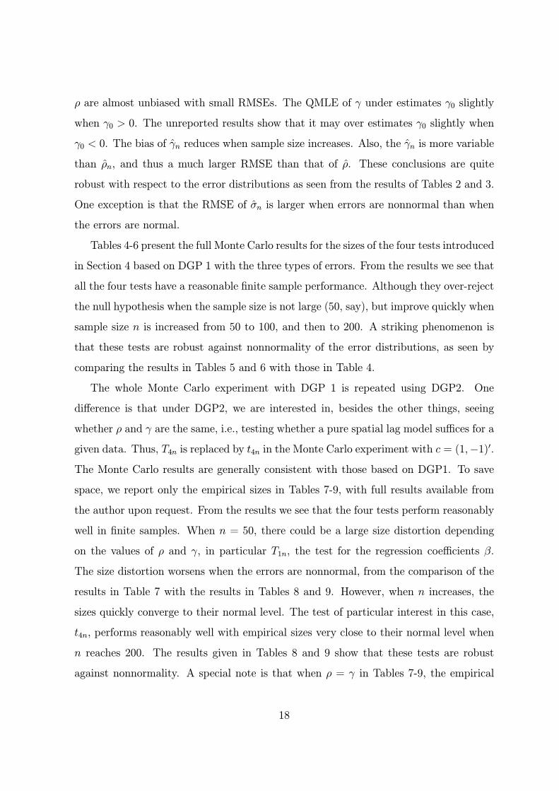
ρ are almost unbiased with small RMSEs. The QMLE of γ under estimates γ0 slightly

when γ0 > 0. The unreported results show that it may over estimates γ0 slightly when

γ0 < 0. The bias of γn reduces when sample size increases. Also, the γn is more variable

than ρn, and thus a much larger RMSE than that of ρ. These conclusions are quite

robust with respect to the error distributions as seen from the results of Tables 2 and 3.

One exception is that the RMSE of σn is larger when errors are nonnormal than when

the errors are normal.

Tables 4-6 present the full Monte Carlo results for the sizes of the four tests introduced

in Section 4 based on DGP 1 with the three types of errors. From the results we see that

all the four tests have a reasonable finite sample performance. Although they over-reject

the null hypothesis when the sample size is not large (50, say), but improve quickly when

sample size n is increased from 50 to 100, and then to 200. A striking phenomenon is

that these tests are robust against nonnormality of the error distributions, as seen by

comparing the results in Tables 5 and 6 with those in Table 4.

The whole Monte Carlo experiment with DGP 1 is repeated using DGP2. One

difference is that under DGP2, we are interested in, besides the other things, seeing

whether ρ and γ are the same, i.e., testing whether a pure spatial lag model suffices for a

given data. Thus, T4n is replaced by t4n in the Monte Carlo experiment with c = (1,−1) .The Monte Carlo results are generally consistent with those based on DGP1. To save

space, we report only the empirical sizes in Tables 7-9, with full results available from

the author upon request. From the results we see that the four tests perform reasonably

well in finite samples. When n = 50, there could be a large size distortion depending

on the values of ρ and γ, in particular T1n, the test for the regression coefficients β.

The size distortion worsens when the errors are nonnormal, from the comparison of the

results in Table 7 with the results in Tables 8 and 9. However, when n increases, the

sizes quickly converge to their normal level. The test of particular interest in this case,

t4n, performs reasonably well with empirical sizes very close to their normal level when

n reaches 200. The results given in Tables 8 and 9 show that these tests are robust

against nonnormality. A special note is that when ρ = γ in Tables 7-9, the empirical

18

sizes correspond to the test for a pure spatial lag model.

6 Conclusions and Discussions

A general model jointly incorporating the local and global spatial externalities in both

modelled and unmodelled effects is introduced. Robust methods of inferences procedures

are developed based on quasi-maximum likelihood estimation method. Simple analytical

forms for the inferential statistics are provided. Large sample properties of the QMLE

are studied. Extensive Monte Carlo simulation shows that the QMLEs of the model

parameters and the tests possess good finite sample properties. The proposed model is

very flexible. The methods of inferences are easy to implement and the tests of spatial

externalities can be easily carried out.

The model can be extended to include regressors of no spatial dependence, and

to allow un to be heteroscedastic. Furthermore, the QMLE is efficient only when the

likelihood is correctly specified. In the absence of knowledge about the error distribution,

it may be possible to extend the adaptive estimation procedure of Robinson (2006) to

improve the efficiency of the QMLEs considered in this paper.

19

Appendix A: Gradient, Hessian and Related Quantities

The gradient function Gn(ξ) =∂∂ξ(ξ) has the elements:

Gnβ(ξ) = 1σ2Xn(ρ)Ω

−1n (γ)εn(β, ρ),

Gnρi(ξ) = 1σ2[Xn,ρi(ρ)β] Ω

−1n (γ)εn(β, ρ), i = 1, · · · , k1,

Gnγi(ξ) = 12σ2

εn(β, ρ)Ω−1n (γ)Ωnγi(γ)Ω

−1n (γ)εn(β, ρ)− 1

2tr[Ω−1n (γ)Ωn,γi(γ)],

i = 1, · · · , k2,Gnσ2(ξ) = 1

2σ4εnΩ

−1n (γ)εn(β, ρ)− n

2σ2.

Note that in the above derivation, we have used the formulas: ∂∂γln |Ωn| = tr(Ω−1n ∂Ωn

∂γ)

and ∂∂γΩ−1n = −Ω−1n ∂Ωn

∂γΩ−1n .

To derive the expression for Kn(ξ0), the variance of Gn(ξ0), recall the notation Zn

and Ω∗n,γi defined in Section 2.3, and use the relations Ωn = BnBn and εn(β0, ρ0) = Bnun.

The gradient function at ξ0 can be written as

Gn(ξ0) =

⎧⎪⎪⎪⎪⎪⎪⎪⎨⎪⎪⎪⎪⎪⎪⎪⎩

1σ20Znun,

12σ20unΩ

∗n,γiun − 1

2tr(Ω∗n,γi), i = 1, · · · , k1,

12σ40unun − n

2σ20.

As the elements of un are iid with mean zero, variance one, skewness α0, and kurtosis

κ0 + 3, the following formulas for conformable matrices Z, Φ1 and Φ2 can easily be

established,

E[(Z un) · (Z un) ] = σ20Z Z,

E[un · (unΦiun)] = σ30α0 daigv(Φi), i = 1, 2,

Cov(unΦiun, unΦjun) = σ40κ0 diagv(Φi) diagv(Φj) + σ40tr(ΦiΦj + ΦiΦj),

for i, j = 1, 2, some simple algebra leads to the expression for Kn(ξ0).

Let Xn,ρiρj(ρ) =∂2

∂ρi∂ρjXn(ρ), and Ωn,γiγj (γ) =

∂2

∂γi∂γjΩn(γ). The Hessian matrix

function Hn(ξ) =∂∂ξGn(ξ) has the elements,

20

Hnββ(ξ) = − 1σ2Xn(ρ)Ω

−1n (γ)Xn(ρ)

Hnβρi(ξ) = 1σ2Xn,ρi(ρ)Ω

−1n (γ)εn(β, ρ)− 1

σ2Xn(ρ)Ω

−1n (γ)Xn,ρi(ρ)β

Hnβγi(ξ) = − 1σ2Xn(ρ)Ω

−1n (γ)Ωn,γi(γ)Ω

−1n (γ)εn(β, ρ)

Hnβσ2(ξ) = − 1σ4Xn(ρ)Ω

−1n (γ)εn(β, ρ)

Hnρiρj(ξ) = 1σ2[Xn,ρiρj (ρ)β] Ω

−1n (γ)εn(β, ρ)− 1

σ2[Xn,ρi(ρ)β] Ω

−1n (γ)Xn,ρj(ρ)β

Hnρiγj (ξ) = − 1σ2[Xn,ρi(ρ)β] Ω

−1n (γ)Ωn,γj (γ)Ω

−1n (γ)εn(β, ρ)

Hnρiσ2(ξ) = − 1σ4[Xn,ρi(ρ)β] Ω

−1n (γ)εn(β, ρ)

Hnγiγj(ξ) = 12tr Ω−1n (γ)Ωn,γj (γ)Ω

−1n (γ)Ωnγi(γ)− Ω−1n (γ)Ωn,γiγj (γ) − 1

2σ2εn(β, ρ)

Ω−1n (γ) 2Ωn,γj(γ)Ω−1n (γ)Ωn,γi(γ)− Ωn,γiγj(γ) Ω−1n (γ)εn(β, ρ)

Hnγiσ2(ξ) = − 12σ4

εn(β, ρ) [Ω−1n (γ)Ωn,γi(γ)Ω

−1n (γ)] εn(β, ρ)

Hnσ2σ2(ξ) = n2σ4− 1

σ6εn(β, ρ) Ω

−1n (γ)εn(β, ρ).

The expected information matrix I(ξ0) = −E[H(ξ0)] has the elements,

In,ββ(ξ0) = 1σ20Xn(ρ0)Ω

−1n (γ)Xn(ρ0) =

1σ20Z1nZ1n,

In,βρ(ξ0) = 1σ20Xn(ρ0)Ω−1n (γ0)Xn,ρi(ρ0)β0 = 1

σ20Z1nZ2n,

In,ρρ(ξ0) = 1σ20

[Xn,ρi(ρ0)β0] Ω−1n (γ0)Xn,ρj (ρ0)β0 = 1

σ20Z2nZ2n,

In,γγ(ξ0) = 12tr Ω−1n (γ0)Ωn,γj(γ0)Ω

−1n (γ0)Ωn,γi(γ0) = 1

2Λn,

In,γσ2(ξ0) = 12σ20tr [Ω−1n (γ0)Ωn,γi(γ0)] =

12σ20Φn1n,

In,σ2σ2(ξ0) = n2σ40,

with the remaining elements being null vectors or matrices.

To derive AVar(βn), AVar(ρn), AVar(γn), and ACov(ρn, γn), given in (15)-(18), note

that Kn(ξ0) = In(ξ0) +K0n, where

K0n =

⎛⎜⎜⎜⎜⎜⎜⎜⎝0, α0

2σ0ZnΦn,

α02σ30Zn1n

∼, κ04ΦnΦn,

κ04σ20Φn1n

∼, ∼, nκ04σ40

⎞⎟⎟⎟⎟⎟⎟⎟⎠ .

21

Partition In(ξ0) and K0n according to (β0, ρ0) and (γ0, σ

20) , and denote the elements of

the partitioned In(ξ0) by I11, I12, I21 and I22, and the elements of the partitioned K0n by

K11, K12, K21 and K22. As I12 = 0, I21 = 0, and K11 = 0, we have

AVar(ξn) = I−1n (ξ0)Kn(ξ0)I−1n (ξ0)

=

⎛⎜⎜⎝ I−111 , 0

0, I−122

⎞⎟⎟⎠+⎛⎜⎜⎝ 0, I−111 K12I

−122

I−122 K21I−111 , I

−122 K22I

−122

⎞⎟⎟⎠which leads immediately to AVar[(βn, ρn) ] = I

−111 = σ20(ZnZn)

−1, and thus the expres-

sions AVar(βn) and AVar(ρn) in (15) and (16).

To derive AVar(γn) given in (17), one needs the upper-left corner submatrix of

I−122 K22I−122 . We have,

I−122 = 2σ20

⎛⎜⎜⎝ σ20Λn, Φn1n

1nΦn,nσ20

⎞⎟⎟⎠−1

=

⎛⎜⎜⎝1σ20Σ−1n , − 1

τnΛ−1n Φn1n

− 1τn1nΦnΛ

−1n ,

σ20τn

⎞⎟⎟⎠ .With

K22 =

⎛⎜⎜⎝κ04ΦnΦn,

κ04σ20Φn1n

∼, nκ04σ40

⎞⎟⎟⎠ ,some simple algebra leads to the expression for AVar(γn).

Finally, to derive ACov(ρn, γn) given in (18), one needs the lower-left corner submatrix

of I−111 K12I−122 . As I

−111 = σ20(Z

−1n Zn)

−1 where Zn = Z1n, Z2n, we obtain,

I−111 = σ20

⎛⎜⎜⎝ (Z1nM2nZ1n)−1, (Z1nZ1n)

−1Z1nZ2n(Z2nM1nZ2n)−1

∼, (Z2nM1nZ2n)−1

⎞⎟⎟⎠Now, K12 = (

α02σ0ZnΦn,

α02σ30Zn1n), which can be written as

K12 =α02σ30

⎛⎜⎜⎝ σ20Z1nΦn, Z1n1n

σ20Z2nΦn, Z2n1n

⎞⎟⎟⎠ .After matrix multiplications, some tedious algebra leads to the expression for ACov(ρn, γn).

22

Appendix B: Detailed Proofs of the Theorems

This appendix presents six lemmas. Lemmas B.1 — B.3 fill in the details for the proof

of Theorem 1, Lemma B.4 gives additional details for proving Theorem 2, and Lemmas

B.5 and B.6 provide details for the proof of Theorem 3. To simplify the proofs of these

lemmas, assume without loss of generality that ρ and γ are both scalars.

Lemma B.1. Under the Assumption 5 and Assumption 7, 1nln |Ω(γ)| is uniformly

equicontinuous in γ ∈ Θ2.

Proof: By the mean value theorem, we have

1

n(ln |Ωn(γ1)|− ln |Ωn(γ2)|) = 1

ntr Ω−1n (γ)Ωnγ(γ) (γ1 − γ2),

where γ lies between γ1 and γ2. As Ωn(γ) = Bn(γ)Bn(γ), Ωn,γ(γ) = Bn,γ(γ)Bn(γ) +

Bn(γ)Bn,γ(γ). As Bn(γ) is uniformly bounded in absolute row sums, uniformly in γ ∈ Θ2(Assumption 5), and the elements of Bn,γ(γ) are uniformly bounded, uniformly in γ ∈ Θ2(Assumption 7), it follows that the elements of Ωnγ(γ) are uniformly bounded, uniformly

in γ ∈ Θ2. Further, as B−1n (γ) is uniformly bounded in absolute row and column

sums, uniformly in γ ∈ Θ2 (Assumption 5), Ω−1n (γ) = B−1n (γ)B −1n (γ) is also uniformly

bounded in absolute row and column sums, uniformly in γ ∈ Θ2.7 It follows that

1ntr [Ω−1n (γ)Ωnγ(γ)] = O(1). Thus,

1nln |Ω(γ)| is uniformly equicontinuous in γ ∈ Θ2. As

Θ2 is a compact set,1n[ln |Ωn(γ1)|− ln |Ωn(γ2)|] = O(1).

Lemma B.2. Under the Assumption 3—8, the σ2n(θ) defined in (12) is uniformly

equicontinuous in θ ∈ Θ.

Proof: By the mean value theorem:

σ2n(θ1)− σ2n(θ2) = σ2nρ(θ)(ρ1 − ρ2) + σ2nγ(θ)(γ1 − γ2),

where θ1 = (ρ1, γ1) , θ2 = (ρ2, γ2) , and θ lies between θ1 and θ2. The partial derivatives

7This follows from a property of the matrix norm as the maximum of the absolute row sums is a

matrix norm. See Horn and Johnson (1985).

23

can be shown, after a lengthy algebra, to have the forms,

σ2nρ(θ) =1

nβ0X (ρ0)Dn(θ)X(ρ0)β0, and

σ2nγ(θ) = −σ20

ntr[Ωn(ρ0)Ω

−1n (γ)Ωn,γ(γ)Ω

−1n (γ)] +

1

nβ0X (ρ0)Fn(θ)X(ρ0)β0

where Dn(θ) = −B −1n (γ)[Rn(θ)M1n(θ) +M1n(θ)Rn(θ)]B−1n (γ),

Rn(θ) = B−1n (γ)An,ρ(ρ)A

−1n (ρ)Bn(γ)[In −M1n(θ)],

Fn(θ) = −B −1n (γ)M1n(θ)B−1n (γ)Ωn,γ(γ)B

−1n (γ)M1n(θ)B

−1n (γ).

As the elements of Xn are uniformly bounded (Assumption 3) and the absolute row sums

of A(ρ) are uniformly bounded (Assumption 4), uniformly in ρ ∈ Θ1, the elements ofXn(ρ) are uniformly bounded, uniformly in ρ ∈ Θ2. The matrices Bn(γ) and B−1n (γ) areuniformly bounded in absolute row and column sums, uniformly in γ ∈ Θ2 (Assumption5), so are the matrices Ωn(γ) and Ω

−1n (γ). It follows that the elements of B

−1n (γ)Xn(ρ)

are uniformly bounded, uniformly in θ ∈ Θ. This together with the Assumption 3 ensurethat the projection matrices M1n(θ) and In−M1n(θ) are uniformly bounded in absolute

row and column sums, uniformly in θ ∈ Θ.8 Thus, the matrices Dn(θ), Rn(θ), and

Fn(θ) are all uniformly bounded in their elements, uniformly in θ in Θ, which leads to

σ2nρ(θ) = O(1) and σ2nγ(θ) = O(1). Thus, σ

2n(θ) is uniformly equicontinuous in θ in Θ.

As Θ is compact, it follows that σ2n(θ1)− σ2n(θ2) = O(1), uniformly in θ1 and θ2 in Θ.

Lemma B.3. Under the Assumption 3—7, the σ2n(θ) defined in (12) is uniformly

bounded away from zero on Θ.

Proof: To prove σ2n(θ) is uniformly bounded away from zero onΘ, and to finally show

the global identifiability of θ0, we employ a similar trick as did Lee (2004b, Appendix B).

Consider an auxiliary model Yn = Bn(γ)un, i.e., a pure spatial error process. We have the

loglikelihood function n,a(γ, σ2) = −n

2ln(2πσ2)− 1

2ln |Ωn(γ)|− 1

2σ2YnΩ

−1n (γ)Yn, and its

expectation n,a(γ,σ2) = −n

2ln(2πσ2) − 1

2ln |Ωn(γ)| − σ20

2σ2tr (Ωn(γ0)Ω

−1(γ)). The latter

is maximized at σ2n,a(γ) =σ20ntr (Ωn(γ0)Ω

−1(γ)), resulting in the concentrated function

8See Lee (2004b, Appendix A) for the proof of a simpler version of this result.

24

cn,a(γ) = −n

2[1 + ln(2π)]− 1

2ln |Ωn(γ)|− n

2ln σ2n,a(γ). We have σ

2n,a(γ0) = σ20, and hence

cn,a(γ0) = −n

2[1 + ln(2π)] − 1

2ln |Ωn(γ0)| − n

2lnσ20. By Jensen’s inequality,

cn,a(γ) =

maxσ2 E[ n,a(γ,σ2)] ≤ E[ n,a(γ0,σ20)] = −n2 ln(2πσ20) − 1

2ln |Ωn(γ0)| − n

2. It follows that

cn,a(γ) ≤ c

n,a(γ0), showing that ln σ2n,a(γ) ≥ 1

n[ln |Ωn(γ0)| + ln |Ωn(γ)|] − lnσ20. Lemma

B.1 shows that 1n[ln |Ωn(γ0)|+ln |Ωn(γ)|] = O(1), hence ln σ2n,a(γ) is bounded from below

uniformly in γ ∈ Θ2. Therefore, σ2n,a(γ) is bounded away from zero, uniformly in γ ∈ Θ2.It follows from (12) that σ2n(θ) is also bounded away from zero, uniformly in θ in Θ.

Lemma B.4. Under Assumptions 1—7, σ2n(θ)− σ2n(θ)p−→ 0, uniformly in θ ∈ Θ.

Proof: First, σ2n(θ) can be rewritten as σ2n(θ) =

1nYnB

−1n (γ)M1n(θ)B

−1n (γ)Yn. With

the true model Yn = Xn(ρ0)β0 +Bn(γ0)un, we have

σ2n(θ) =1

nβ0Xn(ρ0)B

−1n (γ)M1n(θ)B

−1n (γ)Xn(ρ0)β0

+1

nunBn(γ0)B

−1n (γ)M1n(θ)B

−1n (γ)Bn(γ0)un

+2

nβ0Xn(ρ0)B

−1n (γ)M1n(θ)B

−1n (γ)Bn(γ0)un,

and referring to the expression for σ2n(θ) given in (12), we obtain,

σ2n(θ)− σ2n(θ) =1

nunBn(γ0)B

−1n (γ)M1n(θ)B

−1n (γ)Bn(γ0)un −

σ20ntr[Ωn(γ0)Ω

−1n (γ)]

+2

nβ0Xn(ρ0)B

−1n (γ)M1n(θ)B

−1n (γ)Bn(γ0)un.

We show that the last term above is op(1), uniformly in θ ∈ Θ. Assumptions 3 and 4guarantee that the elements of β0Xn(ρ0) are uniformly bounded. As B

−1n (γ) andM1n(θ)

are both uniformly bounded in absolute row and column sums, uniformly in γ ∈ Θ2, orin θ ∈ Θ, the Assumption 1 and an extension of a result of Lee (2004a, Appendix A) tothe case of matrix functions lead to

2

nβ0Xn(ρ0)B

−1n (γ)M1n(θ)B

−1n (γ)Bn(γ0)un = op(1), uniformly in θ ∈ Θ.

Now we show that the difference of the first two terms is op(1). Since B−1n (γ)Bn(γ0) is

uniformly bounded in both absolute row and column sums, it follows from Assumption

25

1 and an extended result of Lee (2004a, Appendix A) that

EunBn(γ0)B −1n (γ)M1n(θ)B−1n (γ)Bn(γ0)un

= σ20tr[B (γ0)B−1n (γ)M1n(θ)B

−1n (γ)Bn(γ0)]

= σ20tr[Bn(γ0)B−1n (γ)B−1n (γ)Bn(γ0)] +O(1)

= σ20tr[Ωn(γ0)Ω−1n (γ)] +O(1)

and that

VarunBn(γ0)B −1n (γ)M1n(θ)B−1n (γ)Bn(γ0)un

= σ40κ0 diagv[Rn(θ)] diagv[Rn(θ)] + 2σ40tr[R

2n(θ)],

where Rn(θ) = Bn(γ0)B−1n (γ)M1n(θ)B

−1n (γ)Bn(γ0). Now, it is easy to show that Rn(θ)

is uniformly bounded in absolute row and column sums, uniformly in θ ∈ Θ. Hence,by a matrix norm property, Rn(θ)Rn(θ) is also uniformly bounded in absolute row and

column sums, uniformly in θ ∈ Θ. It follows that the elements of R2n are uniformlybounded, uniformly in θ ∈ Θ. Hence,

VarunBn(γ0)B −1n (γ)M1n(θ)B−1n (γ)Bn(γ0)un = O(n),

uniformly in θ ∈ Θ. Finally, Chebyshev’s inequality leads to1

nunBn(γ0)B

−1n (γ)M1n(θ)B

−1n (γ)Bn(γ0)un −

σ20ntr[Ωn(γ0)Ω

−1n (γ)] = op(1),

which gives σ2n(θ)− σ2n(θ) = op(1) and hence the consistency of the QMLE ξn of ξ0.

Lemma B.5. Under the Assumptions 1-10, we have 1n[Hn(ξn)−Hn(ξ0)] = op(1).

Proof: As ξn −→ ξ0, ξn −→ ξ0. As Hn(ξn) is either linear or quadratic in βn, and is

linear in σ−kn , k = 2, 4, or 6. As βn = β0 + op(1) and σ−kn = σ−k0 + op(1), we have,

1

nHn(ξn) =

1

nHn(β0, θn, σ

20) + op(1)

=1

nHn(ξ0) +

1

n

∂

∂ρnHn(β0, θn,σ

20)(ρn − ρ0) +

1

n

∂

∂γnHn(β0, θn, σ

20)(γn − γ0) + op(1),

where θn lies between θn and θ0, and the second equation follows from the mean value

theorem. Under the Assumptions 9 and 10, it is easy to show that 1n

∂∂ρnHn(β0, θn,σ

20) =

Op(1) and1n

∂∂γnHn(β0, θn,σ

20) = Op(1). The result of Lemma 5 thus follows.

26

Lemma B.6. Under the Assumptions 1-10, we have 1n[Hn(ξ0) + In(ξ0)] = op(1).

Proof: From Appendix A, we have,

Hn(ξ0) + In(ξ0) =

⎛⎜⎜⎜⎜⎜⎜⎜⎜⎜⎜⎜⎝

0, 1σ20(B−1n Xnρ) un, − 1

σ20Z1nΩ

∗nγun, − 1

σ40Z1nun

∼, 1σ20(B−1n Xnρρ) un, − 1

σ20Z2nΩ

∗nγun, − 1

σ40Z2nun

∼, ∼, q1(un) + q2(un), q3(un)

∼, ∼, ∼ q4(un)

⎞⎟⎟⎟⎟⎟⎟⎟⎟⎟⎟⎟⎠where q1(un) = tr(Ω

∗2nγ) − 1

σ20unΩ

∗2nγun, q2(un) =

12σ20unB

−1n ΩnγγB

−1n un − 1

2tr(Ω−1n Ωnγγ),

q3(un) =1σ20tr(Ω∗nγ) − 1

σ40unΩ

∗nγun, and q4(un) =

nσ40− 1

σ60unun. Thus, the elements of

Hn(ξ0) + In(ξ0) are either linear or quadratic forms of un, which can easily be shown to

be op(n) by applying the Chebyshev’s inequality. The result of Lemma 6 follows.

27

References

Abbot, A. (1997). Of time and space: the contemporary relevance of the Chicago

school. Social Forces 75, 1149-1182.

Akerlof, G. A. (1997). Social distance and social decisions. Econometrica 65 1005-1027.

Anselin, L. (1988). Spatial Econometrics: Methods and Models. Dordrecht, the Nether-

lands: Kluwer.

Anselin, L. (2001). Spatial econometrics. InA Companion to Theoretical Econometrics,

ed. by B. H. Baltagi. Oxford: Blackwell.

Anselin, L. (2003). Spatial externalities, spatial multipliers, and spatial econometrics.

International Regional Science Review 26, 153-166.

Anselin, L. and Bera, A. K. (1998). Spatial dependence in linear regression models

with an introduction to spatial econometrics. In Handbook of Applied Economic

Statistics, ed. by A. Ullah and D. E. A. Giles. New York: Marcel Dekker.

Besley, T. and Case, A. C. (1995). Incumbent behavior: vote-seeking, tax-setting, and

yardstick competition. American Economic Review 85, 25-45.

Benirschka, M. and Binkley, J. K. (1994). Land price volatility in a geographically

dispersed market. American Journal of Agricultural Economics 76, 185-195.

Case, A. (1991). Spatial patterns in household demand. Econometrica 59, 953-965.

Case, A. (1992). Neighborhood influence and technological change. Regional Science

and Urban Economics 22, 491-508.

Case, A., Rosen, H. S. and Hines, J. R. (1993). Budget spillovers and fiscal Policy

interdependence: evidence from the states. Journal of Public Economics 52, 285-

307.

Cliff and Ord (1981). Spatial Processes: Models and Applications. London: Pion.

Elhorst, J. P. (2003). Specification and Estimation of Spatial Panel Data Models.

International Regional Science Review 26, 244-268.

Glaeser, E. L. Sacerdote, B. and Scheinkman, J. (1996). Crime and social interactions.

Quarterly Journal of Economics 111, 507-548.

28

Goodchild, M., Anselin, L, Appelbaum, R and Harthorn, B (2000). Toward spatially

integrated social science. International Regional Science Review 23, 139-159.

Griffith, D. A. (1988). Advanced Spatial Statistics. Dordrecht, the Netherlands: Kluwer.

Haining, R. (1990). Spatial Data Analysis in the Social and Environmental Sciences.

Cambridge: Cambridge University Press.

Horn, R. A. and Johnson C. R. (1985). Matrix Analysis. Cambridge: Cambridge

University Press.

Huang, J. S. (1984). The autoregressive moving average model for spatial analysis.

Australian Journal of Statistics 26, 169-178.

Kelejian, H. H. and Prucha, I. R. (1998). A generalized spatial two-stage least squares

procedure for estimating a spatial autoregressive model with autoregressive dis-

turbances. Journal of Real Estate Finance and Economisc 17, 99-121.

Kelejian, H. H. and Prucha, I. R. (1999). A generalized moment estimator for the

autoregressive parameter in a spatial model. International Economic Review 40,

509-533.

Kelejian, H. H. and Prucha, I. R. (2001). On the asymptotic distribution of the Moran

it I test statistic with applications. Journal of Econometrics 104, 219-257.

Kelejian, H. H. and Prucha, I. R. (2006). Specification and estimation of spatial au-

toregressive models with autoregressive and heteroskedastic disturbances. Working

paper, Department of Economics, University of Maryland.

Lee, L. F. (2002). Consistency and efficiency of least squares estimation for mixed

regressive, spatial autoregressive models. Econometric Theory 18, 252-277.

Lee, L. F. (2004a). Asymptotic distributions of quasi-maximum likelihood estimators

for spatial autoregressive models. Econometrica 72, 1899-1925.

Lee, L. F. (2004b). Asymptotic distributions of quasi-maximum likelihood estimators

for spatial autoregressive models, and Appendix, April 2004. Working Paper,

http://economics.sbs.ohio-state.edu/lee/.

LeSage J. P. (1999). The Theory and Practice of Spacial Econometrics. Manual in

http://www.spatial-econometrics.com

29

Magnus, J. R. (1982). Multivariate error components analysis of linear and nonlinear

regression models by maximum likelihood. Journal of Econometrics 19, 239-285.

Magnus, J. R. and Neudecker, H. (1999). Matrix Differential Calculus with Applications

in Statistics and Econometrics, Revised Edition. John Wiley & Sons.

Robinson, P. M. (2006). Efficient Estimation of the Semiparametric Spatial Auture-

gressive Model. Working Paper, London School of Economics.

Sampson, R. A. Morenoff, J. and Earls, F. (1999). Beyond social capital: spatial

dynamics and collective efficacy for children. American Sociological Review 64,

633-660.

White, H. (1996). Estimation, Inference and Specification Analysis. New York: Cam-

bridge University Press.

30

Table 1. Mean and RMSE for the QMLEs, DGP1 with Normal Errorsn = 50, 100, and 200, for upper, middle and lower panels, respectively

MC Estimate of Mean MC Estimate of RMSEρ γ β0 β1 β2 σ ρ γ β0 β1 β2 σ ρ γ.0 .0 5.000 2.000 2.000 .934 .001 -.041 .178 .048 .050 .121 .029 .199

.2 5.003 1.999 1.999 .944 -.001 .150 .206 .051 .050 .115 .029 .199

.5 5.015 1.998 2.000 .943 -.001 .433 .300 .052 .050 .118 .029 .181

.8 5.006 2.000 2.001 .958 -.001 .740 .755 .056 .052 .113 .030 .132.2 .0 5.002 2.000 2.001 .936 .200 -.046 .155 .049 .048 .120 .030 .198

.2 4.998 2.000 1.999 .940 .200 .142 .171 .051 .048 .118 .028 .203

.5 4.999 1.998 2.001 .944 .200 .433 .254 .054 .052 .115 .028 .185

.8 5.002 2.002 2.002 .961 .199 .741 .639 .058 .053 .115 .027 .131.5 .0 5.002 1.999 2.001 .936 .500 -.047 .133 .048 .047 .118 .032 .202

.2 5.004 1.999 2.000 .941 .500 .144 .143 .048 .049 .118 .028 .203

.5 5.006 1.999 2.000 .948 .499 .428 .199 .053 .053 .115 .026 .183

.8 4.991 2.001 2.001 .958 .501 .734 .529 .062 .056 .112 .026 .136.8 .0 5.005 2.001 2.000 .938 .800 -.047 .114 .045 .046 .118 .034 .197

.2 4.998 2.000 2.000 .943 .800 .132 .121 .045 .048 .117 .030 .202

.5 5.002 2.003 2.001 .950 .800 .439 .174 .052 .051 .115 .026 .176

.8 4.992 2.001 2.000 .961 .799 .735 .416 .059 .056 .110 .024 .134.0 .0 5.005 1.999 2.001 .972 .000 -.013 .185 .035 .036 .075 .025 .138

.2 4.999 2.000 2.002 .972 .000 .175 .203 .035 .036 .076 .026 .137

.5 5.004 2.000 1.999 .974 -.000 .476 .252 .036 .036 .076 .026 .116

.8 5.010 1.999 1.998 .979 -.002 .773 .519 .037 .038 .078 .028 .075.2 .0 5.001 2.001 1.999 .970 .200 -.022 .151 .034 .035 .075 .025 .137

.2 5.003 1.999 2.000 .969 .200 .176 .158 .035 .037 .077 .024 .133

.5 5.014 2.000 1.999 .974 .199 .473 .210 .037 .039 .078 .025 .114

.8 5.003 2.001 2.000 .984 .200 .771 .428 .038 .040 .078 .025 .076.5 .0 5.004 1.999 2.000 .971 .500 -.021 .121 .034 .035 .075 .025 .136

.2 5.003 2.000 2.000 .967 .500 .175 .125 .036 .036 .078 .024 .137

.5 5.002 1.999 2.000 .973 .500 .469 .159 .038 .040 .077 .022 .120

.8 5.006 2.000 2.000 .982 .499 .770 .347 .040 .042 .076 .023 .076.8 .0 5.004 1.999 2.000 .968 .799 -.023 .101 .034 .034 .078 .026 .137

.2 5.005 1.999 2.000 .970 .799 .171 .106 .037 .036 .075 .024 .131

.5 5.001 2.000 2.000 .972 .800 .473 .137 .037 .038 .079 .022 .115

.8 4.995 2.002 2.000 .982 .800 .768 .297 .041 .044 .077 .021 .080.0 .0 5.001 1.999 2.000 .984 -.000 -.009 .110 .025 .028 .053 .017 .095

.2 5.007 2.000 2.000 .986 -.001 .189 .121 .025 .028 .053 .018 .091

.5 4.994 2.000 2.000 .985 .001 .487 .166 .026 .029 .054 .018 .080

.8 5.009 2.000 2.001 .988 .000 .786 .359 .027 .029 .054 .018 .049.2 .0 5.005 2.000 1.999 .985 .200 -.006 .095 .025 .028 .053 .018 .099

.2 5.005 2.001 2.000 .987 .199 .187 .099 .024 .028 .052 .018 .095

.5 4.999 2.001 2.001 .987 .200 .488 .139 .027 .029 .054 .017 .076

.8 5.005 2.001 2.000 .989 .200 .786 .296 .028 .030 .052 .017 .048.5 .0 5.000 1.999 2.001 .984 .500 -.010 .073 .023 .028 .052 .018 .095

.2 4.998 2.000 2.000 .984 .500 .184 .080 .025 .028 .053 .017 .095

.5 5.001 2.001 2.000 .987 .500 .482 .106 .027 .031 .052 .016 .081

.8 5.000 2.000 1.998 .990 .500 .785 .246 .029 .032 .054 .015 .049.8 .0 5.001 2.000 1.999 .984 .800 -.011 .064 .023 .027 .054 .019 .096

.2 5.003 2.000 1.999 .985 .799 .183 .067 .024 .028 .053 .017 .096

.5 5.007 2.000 2.000 .989 .799 .480 .091 .027 .032 .052 .015 .080

.8 5.002 2.000 2.000 .992 .800 .785 .200 .031 .034 .054 .014 .049

31

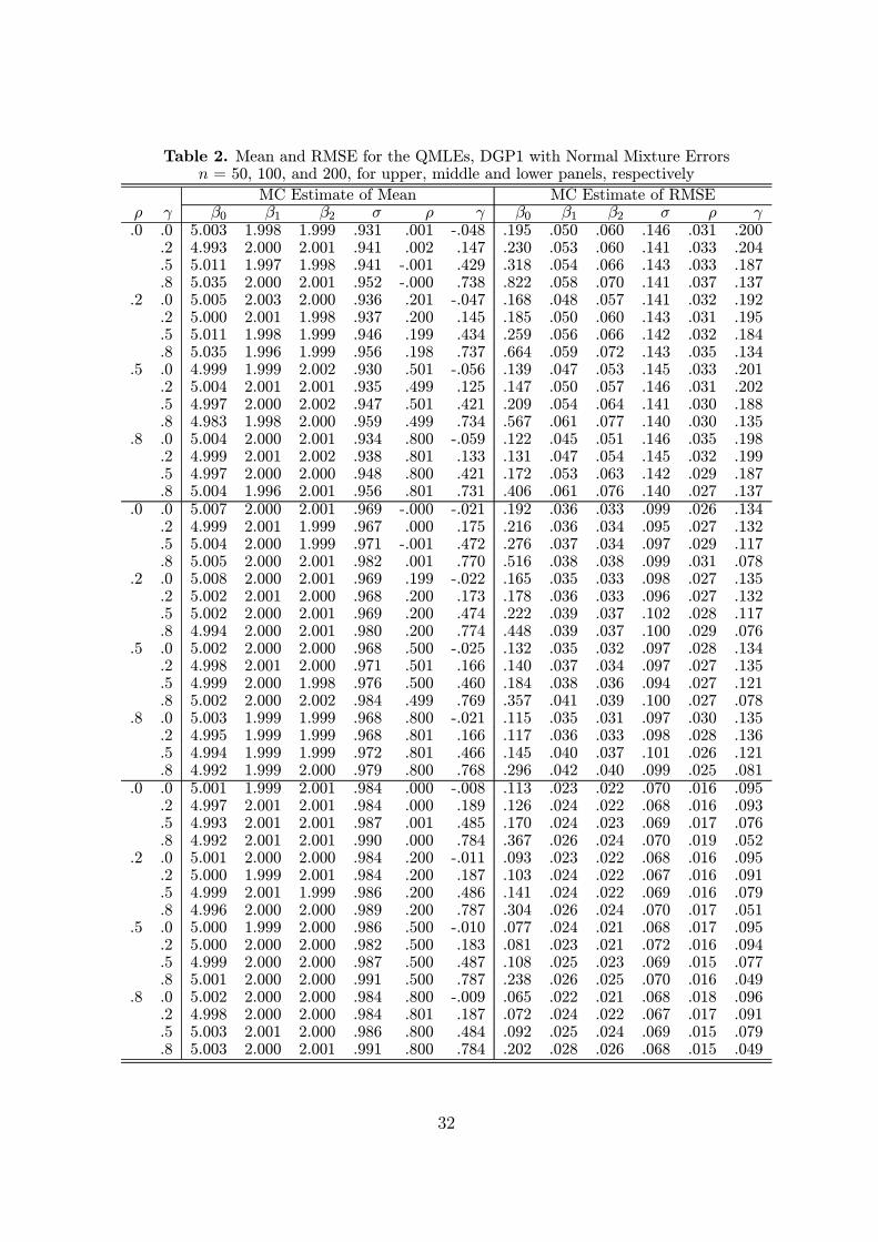
Table 2. Mean and RMSE for the QMLEs, DGP1 with Normal Mixture Errorsn = 50, 100, and 200, for upper, middle and lower panels, respectively

MC Estimate of Mean MC Estimate of RMSEρ γ β0 β1 β2 σ ρ γ β0 β1 β2 σ ρ γ.0 .0 5.003 1.998 1.999 .931 .001 -.048 .195 .050 .060 .146 .031 .200

.2 4.993 2.000 2.001 .941 .002 .147 .230 .053 .060 .141 .033 .204

.5 5.011 1.997 1.998 .941 -.001 .429 .318 .054 .066 .143 .033 .187

.8 5.035 2.000 2.001 .952 -.000 .738 .822 .058 .070 .141 .037 .137.2 .0 5.005 2.003 2.000 .936 .201 -.047 .168 .048 .057 .141 .032 .192

.2 5.000 2.001 1.998 .937 .200 .145 .185 .050 .060 .143 .031 .195

.5 5.011 1.998 1.999 .946 .199 .434 .259 .056 .066 .142 .032 .184

.8 5.035 1.996 1.999 .956 .198 .737 .664 .059 .072 .143 .035 .134.5 .0 4.999 1.999 2.002 .930 .501 -.056 .139 .047 .053 .145 .033 .201

.2 5.004 2.001 2.001 .935 .499 .125 .147 .050 .057 .146 .031 .202

.5 4.997 2.000 2.002 .947 .501 .421 .209 .054 .064 .141 .030 .188

.8 4.983 1.998 2.000 .959 .499 .734 .567 .061 .077 .140 .030 .135.8 .0 5.004 2.000 2.001 .934 .800 -.059 .122 .045 .051 .146 .035 .198

.2 4.999 2.001 2.002 .938 .801 .133 .131 .047 .054 .145 .032 .199

.5 4.997 2.000 2.000 .948 .800 .421 .172 .053 .063 .142 .029 .187

.8 5.004 1.996 2.001 .956 .801 .731 .406 .061 .076 .140 .027 .137.0 .0 5.007 2.000 2.001 .969 -.000 -.021 .192 .036 .033 .099 .026 .134

.2 4.999 2.001 1.999 .967 .000 .175 .216 .036 .034 .095 .027 .132

.5 5.004 2.000 1.999 .971 -.001 .472 .276 .037 .034 .097 .029 .117

.8 5.005 2.000 2.001 .982 .001 .770 .516 .038 .038 .099 .031 .078.2 .0 5.008 2.000 2.001 .969 .199 -.022 .165 .035 .033 .098 .027 .135

.2 5.002 2.001 2.000 .968 .200 .173 .178 .036 .033 .096 .027 .132

.5 5.002 2.000 2.001 .969 .200 .474 .222 .039 .037 .102 .028 .117

.8 4.994 2.000 2.001 .980 .200 .774 .448 .039 .037 .100 .029 .076.5 .0 5.002 2.000 2.000 .968 .500 -.025 .132 .035 .032 .097 .028 .134

.2 4.998 2.001 2.000 .971 .501 .166 .140 .037 .034 .097 .027 .135

.5 4.999 2.000 1.998 .976 .500 .460 .184 .038 .036 .094 .027 .121

.8 5.002 2.000 2.002 .984 .499 .769 .357 .041 .039 .100 .027 .078.8 .0 5.003 1.999 1.999 .968 .800 -.021 .115 .035 .031 .097 .030 .135

.2 4.995 1.999 1.999 .968 .801 .166 .117 .036 .033 .098 .028 .136

.5 4.994 1.999 1.999 .972 .801 .466 .145 .040 .037 .101 .026 .121

.8 4.992 1.999 2.000 .979 .800 .768 .296 .042 .040 .099 .025 .081.0 .0 5.001 1.999 2.001 .984 .000 -.008 .113 .023 .022 .070 .016 .095

.2 4.997 2.001 2.001 .984 .000 .189 .126 .024 .022 .068 .016 .093

.5 4.993 2.001 2.001 .987 .001 .485 .170 .024 .023 .069 .017 .076

.8 4.992 2.001 2.001 .990 .000 .784 .367 .026 .024 .070 .019 .052.2 .0 5.001 2.000 2.000 .984 .200 -.011 .093 .023 .022 .068 .016 .095

.2 5.000 1.999 2.001 .984 .200 .187 .103 .024 .022 .067 .016 .091

.5 4.999 2.001 1.999 .986 .200 .486 .141 .024 .022 .069 .016 .079

.8 4.996 2.000 2.000 .989 .200 .787 .304 .026 .024 .070 .017 .051.5 .0 5.000 1.999 2.000 .986 .500 -.010 .077 .024 .021 .068 .017 .095

.2 5.000 2.000 2.000 .982 .500 .183 .081 .023 .021 .072 .016 .094

.5 4.999 2.000 2.000 .987 .500 .487 .108 .025 .023 .069 .015 .077

.8 5.001 2.000 2.000 .991 .500 .787 .238 .026 .025 .070 .016 .049.8 .0 5.002 2.000 2.000 .984 .800 -.009 .065 .022 .021 .068 .018 .096

.2 4.998 2.000 2.000 .984 .801 .187 .072 .024 .022 .067 .017 .091

.5 5.003 2.001 2.000 .986 .800 .484 .092 .025 .024 .069 .015 .079

.8 5.003 2.000 2.001 .991 .800 .784 .202 .028 .026 .068 .015 .049

32

Table 3. Mean and RMSE for the QMLEs, DGP1 with Normal-Gamma Mixture Errorsn = 50, 100, and 200, for upper, middle and lower panels, respectively

MC Estimate of Mean MC Estimate of RMSEρ γ β0 β1 β2 σ ρ γ β0 β1 β2 σ ρ γ.0 .0 5.007 2.001 2.000 .938 -.000 -.037 .222 .056 .064 .146 .035 .193

.2 5.007 2.000 1.999 .935 -.000 .158 .235 .057 .064 .142 .034 .193

.5 5.020 1.998 1.997 .943 -.002 .444 .323 .059 .065 .147 .035 .175

.8 5.042 2.000 2.000 .945 -.000 .747 .821 .060 .070 .142 .036 .125.2 .0 5.008 1.999 1.998 .935 .199 -.032 .176 .056 .064 .143 .032 .199

.2 5.002 1.999 2.001 .935 .200 .151 .198 .059 .066 .149 .032 .201

.5 4.992 2.000 2.000 .945 .200 .437 .268 .060 .067 .145 .032 .178

.8 5.008 1.999 2.002 .955 .200 .745 .723 .063 .072 .144 .033 .127.5 .0 5.005 2.000 2.000 .938 .499 -.051 .136 .053 .062 .147 .032 .202

.2 5.002 2.000 2.000 .941 .500 .150 .149 .056 .065 .144 .030 .193

.5 5.001 1.999 1.999 .945 .500 .436 .213 .060 .070 .142 .027 .174

.8 5.003 1.998 1.999 .956 .498 .739 .550 .065 .073 .140 .027 .131.8 .0 5.001 1.999 1.999 .938 .799 -.034 .115 .052 .059 .147 .031 .189

.2 5.010 2.001 1.996 .941 .799 .148 .121 .053 .065 .142 .028 .198

.5 5.012 2.000 2.002 .947 .800 .440 .171 .061 .071 .141 .025 .182

.8 5.001 2.000 2.002 .959 .801 .736 .407 .067 .076 .140 .023 .134.0 .0 5.007 2.000 2.000 .965 .000 -.014 .140 .037 .042 .099 .023 .138

.2 4.998 2.001 2.000 .968 .001 .179 .149 .036 .043 .101 .022 .135

.5 5.008 2.000 2.000 .972 -.001 .475 .220 .039 .044 .099 .023 .114

.8 5.014 2.000 2.000 .976 -.000 .774 .508 .042 .045 .101 .025 .077.2 .0 5.005 2.001 2.002 .964 .199 -.017 .116 .036 .043 .099 .023 .134

.2 5.000 2.000 1.999 .971 .200 .176 .131 .037 .043 .102 .023 .136

.5 5.001 2.000 2.001 .974 .200 .468 .175 .038 .044 .096 .022 .120

.8 5.002 2.000 2.000 .979 .199 .773 .415 .041 .046 .100 .022 .076.5 .0 4.994 1.999 2.000 .965 .501 -.017 .098 .034 .042 .099 .024 .134

.2 4.999 2.001 1.999 .971 .500 .173 .108 .036 .043 .099 .023 .134

.5 5.010 2.001 2.000 .975 .499 .464 .147 .040 .046 .099 .021 .121

.8 5.014 2.000 2.001 .982 .500 .771 .365 .045 .049 .101 .020 .077.8 .0 5.000 2.001 2.000 .967 .801 -.021 .086 .034 .041 .097 .026 .137

.2 4.997 2.001 1.999 .968 .801 .170 .092 .036 .044 .098 .023 .133

.5 5.002 2.002 2.000 .971 .800 .466 .121 .040 .048 .101 .020 .118

.8 5.004 2.000 2.001 .978 .801 .771 .281 .047 .052 .101 .018 .075.0 .0 5.003 2.001 2.001 .982 -.000 -.006 .118 .027 .021 .069 .017 .096

.2 5.004 1.999 2.000 .982 .000 .189 .128 .026 .022 .070 .017 .095

.5 5.005 2.000 2.000 .989 .000 .486 .173 .026 .023 .071 .017 .078

.8 4.996 2.000 2.000 .989 .000 .788 .361 .026 .023 .072 .018 .048.2 .0 4.998 1.999 1.999 .984 .201 -.011 .097 .026 .022 .069 .017 .095

.2 4.998 2.000 2.000 .984 .200 .188 .105 .027 .022 .071 .017 .094

.5 4.999 1.999 2.001 .986 .200 .486 .141 .027 .023 .070 .016 .077

.8 5.000 2.000 2.000 .989 .201 .788 .299 .028 .023 .074 .016 .048.5 .0 5.003 2.000 2.000 .982 .500 -.010 .080 .026 .021 .070 .018 .094

.2 5.001 2.000 2.000 .983 .499 .186 .086 .027 .022 .070 .017 .093

.5 5.003 2.000 2.000 .984 .500 .487 .110 .028 .023 .069 .016 .078

.8 5.006 1.999 1.999 .989 .499 .786 .248 .029 .025 .072 .015 .050.8 .0 5.003 2.000 1.999 .985 .800 -.014 .067 .024 .021 .071 .018 .095

.2 4.998 2.000 2.000 .984 .801 .185 .071 .027 .022 .068 .017 .095

.5 5.003 2.000 2.000 .986 .799 .483 .093 .029 .024 .070 .015 .077

.8 4.997 1.999 2.000 .989 .800 .784 .202 .031 .025 .071 .014 .049

33

Table 4. Empirical Sizes (%) for the Four Tests, DGP1 with Normal Errors

n = 50 n = 100 n = 200ρ0 γ0 T1n T2n T3n T4n T1n T2n T3n T4n T1n T2n T3n T4n-.8 -.8 8.55 7.75 8.15 9.15 6.60 6.75 6.75 7.85 6.10 5.45 4.90 5.30

-.5 9.55 8.30 10.15 11.65 6.95 6.45 6.90 7.35 6.10 6.30 6.30 6.75-.2 9.80 6.80 11.20 10.60 6.85 7.05 6.60 7.65 6.80 5.95 5.50 5.70.0 9.80 8.55 10.60 13.05 6.90 7.50 6.70 8.05 5.90 5.30 7.10 7.10.2 9.30 9.40 9.85 12.70 7.20 6.30 6.85 7.60 6.50 5.95 6.50 6.60.5 12.05 9.75 12.55 14.10 8.10 7.40 6.95 8.00 5.85 6.10 6.40 6.50.8 12.70 8.20 9.75 11.20 7.75 6.25 7.30 7.45 6.35 5.95 6.00 6.90

-.5 -.8 9.80 8.55 8.45 10.20 7.05 5.35 7.40 6.85 6.90 5.90 5.30 5.90-.5 10.80 8.15 10.60 10.70 6.75 6.05 6.40 7.55 6.10 6.10 6.15 6.05-.2 10.25 8.10 11.40 12.30 6.65 6.05 8.00 7.30 5.55 5.80 6.10 6.90.0 9.65 7.60 9.75 11.05 8.40 7.40 6.60 7.75 6.00 6.30 6.65 7.30.2 10.50 7.85 10.75 11.00 6.95 5.80 6.90 7.60 5.80 5.40 5.75 5.45.5 10.80 8.20 8.85 10.40 7.20 5.95 6.90 6.55 6.00 5.20 6.20 6.55.8 15.00 7.15 12.20 13.10 8.80 6.30 7.70 7.60 7.70 6.15 5.60 6.15

-.2 -.8 9.95 7.40 7.55 8.70 7.05 5.85 6.65 7.10 6.75 5.50 6.75 6.35-.5 10.80 8.25 9.70 11.35 7.10 5.60 6.55 6.70 5.30 5.05 5.75 5.90-.2 10.35 8.40 10.65 11.40 6.40 6.20 6.80 7.15 6.20 5.15 6.70 6.70.0 9.65 7.40 11.40 11.85 5.95 5.55 6.55 6.35 6.95 5.50 5.60 5.50.2 9.35 7.65 9.30 10.55 7.15 6.75 7.25 7.15 5.50 5.15 4.80 5.15.5 10.90 7.05 9.15 10.35 7.45 6.80 6.50 6.85 6.25 5.70 4.80 5.35.8 13.45 8.05 10.15 11.00 9.50 6.20 7.00 8.05 7.65 5.45 6.45 6.05

.0 -.8 8.65 7.95 7.30 8.75 7.20 5.95 6.50 6.95 6.30 5.55 5.65 5.85-.5 10.15 8.50 11.50 12.00 6.40 6.60 6.60 7.65 5.80 5.50 5.80 5.70-.2 9.25 7.80 11.90 12.00 6.90 6.85 7.15 8.25 5.30 5.25 6.65 6.30.0 9.60 7.70 10.25 10.70 6.80 5.40 7.70 7.20 6.40 5.25 6.05 6.45.2 10.45 7.40 9.95 10.15 7.30 5.80 7.60 7.95 5.65 5.90 5.60 5.05.5 11.40 7.55 8.30 9.60 6.45 5.20 6.00 6.10 6.90 5.95 6.50 6.65.8 14.10 6.65 9.50 9.90 9.85 6.80 6.45 6.90 7.50 5.10 5.90 5.35

.2 -.8 9.00 6.85 8.40 9.40 6.60 5.55 6.45 6.70 6.80 5.05 6.20 5.80-.5 10.45 8.25 10.00 11.30 6.30 5.80 7.90 8.75 6.10 5.50 6.10 6.20-.2 9.30 6.70 11.30 11.10 6.65 4.65 7.55 7.70 6.65 5.85 6.75 6.30.0 10.60 7.10 10.45 10.60 6.80 6.20 7.20 7.15 6.30 6.25 7.05 7.40.2 9.70 6.95 10.10 10.25 6.25 6.65 5.90 7.15 5.05 6.15 6.60 6.95.5 11.85 7.40 9.30 9.25 7.70 6.55 6.35 7.10 6.45 5.60 4.75 6.10.8 14.05 6.95 9.95 9.75 9.00 5.20 6.05 6.50 7.40 6.05 5.45 5.45

.5 -.8 8.55 7.50 7.65 9.00 8.00 6.85 6.80 8.30 6.00 4.90 5.70 5.80-.5 10.75 7.90 10.45 10.95 7.40 6.15 7.25 8.40 6.15 6.65 5.90 6.70-.2 9.25 7.30 9.30 9.90 6.95 6.05 6.75 7.05 5.75 4.95 5.70 6.40.0 10.25 7.65 11.10 11.75 6.90 5.50 6.40 7.20 6.20 4.70 5.30 5.25.2 11.20 6.80 10.85 10.65 7.20 6.85 7.80 8.35 6.25 6.15 6.70 6.40.5 12.30 7.05 9.70 9.25 6.65 5.90 6.95 7.90 6.00 5.80 6.95 6.80.8 17.00 6.95 9.60 9.10 10.60 5.65 5.70 6.00 7.30 4.75 5.55 5.30

.8 -.8 9.20 8.20 9.05 10.30 7.70 7.30 6.15 7.50 6.80 5.95 5.95 6.65-.5 10.25 7.85 10.25 11.20 8.10 7.15 7.25 8.00 6.50 6.05 6.05 6.35-.2 10.85 8.15 9.80 11.80 8.00 5.75 7.90 8.05 5.55 5.85 6.75 6.70.0 10.55 7.55 10.50 10.60 7.30 6.35 7.70 7.70 7.60 5.75 6.25 6.10.2 10.30 6.80 9.30 9.65 7.85 6.15 6.10 7.10 5.80 5.60 6.60 7.05.5 12.80 6.00 8.65 8.85 6.15 6.55 6.35 7.35 7.05 5.25 5.70 5.50.8 15.40 6.80 8.55 8.80 9.35 5.85 6.50 6.70 7.70 5.55 4.55 5.60

34

Table 5. Empirical Sizes (%), DGP1 with Normal Mixture Errors

n = 50 n = 100 n = 200ρ0 γ0 T1n T2n T3n T4n T1n T2n T3n T4n T1n T2n T3n T4n-.8 -.8 9.60 7.80 7.65 9.10 6.35 6.20 6.35 7.00 5.25 5.35 5.60 5.70

-.5 10.45 6.60 10.40 10.85 7.75 6.90 7.30 8.55 6.15 4.30 5.60 5.95-.2 10.50 8.25 9.55 10.95 7.80 7.25 6.55 7.05 6.90 5.65 5.75 6.50.0 9.95 8.15 9.75 11.10 7.55 7.15 6.75 7.80 6.50 6.60 5.55 6.75.2 10.20 10.05 9.85 12.20 6.20 7.45 6.75 8.80 5.65 5.45 5.60 6.20.5 11.25 9.55 10.80 13.10 8.05 7.45 6.95 7.80 6.45 7.15 5.20 7.05.8 10.15 8.20 9.70 11.20 8.00 6.50 7.30 9.20 6.55 5.30 6.30 6.45

-.5 -.8 8.85 7.60 8.05 9.60 6.45 5.75 6.15 6.75 5.35 5.40 5.50 5.35-.5 8.20 7.30 9.10 9.70 7.00 6.15 7.10 7.05 5.85 4.40 5.50 5.85-.2 9.90 7.85 8.75 10.25 8.45 6.75 7.55 8.80 5.95 5.55 5.05 6.10.0 8.40 7.55 9.90 11.10 7.80 5.60 7.75 7.20 5.65 5.10 5.65 6.45.2 10.85 7.90 8.95 10.10 7.15 5.95 6.15 6.45 5.85 5.00 5.65 5.90.5 10.75 8.55 8.60 9.75 7.95 7.00 5.60 6.65 4.95 5.80 6.00 6.45.8 13.85 7.00 12.45 13.10 7.85 6.85 7.45 8.75 8.15 4.70 5.60 5.45

-.2 -.8 8.15 5.85 7.65 8.25 7.20 6.15 5.60 6.75 6.15 5.55 5.05 5.15-.5 8.70 6.80 8.95 9.90 7.20 5.70 7.30 7.35 6.95 5.80 5.55 6.20-.2 9.65 7.95 9.95 11.10 7.85 6.40 6.80 6.85 5.75 5.60 5.30 5.45.0 9.30 8.30 10.45 11.15 6.95 6.05 7.55 7.45 6.95 5.65 6.10 5.70.2 10.85 7.65 10.65 12.20 7.65 7.15 6.65 7.95 6.25 5.75 5.60 5.85.5 10.45 9.45 10.00 11.70 7.00 6.80 5.90 6.95 6.50 5.60 5.70 6.40.8 13.90 7.70 10.80 11.90 8.20 5.85 6.65 7.70 7.65 5.35 6.15 6.00

.0 -.8 9.00 6.35 7.35 8.95 6.10 5.50 5.95 6.25 6.10 6.10 5.55 6.05-.5 9.65 7.25 9.45 10.35 7.00 5.25 6.35 6.40 6.05 5.70 6.05 6.65-.2 9.75 7.75 9.60 10.85 7.40 6.80 7.45 8.80 5.45 5.35 5.60 5.60.0 9.95 7.35 10.30 11.10 6.45 4.80 6.85 6.65 5.80 5.65 5.55 5.85.2 10.35 9.15 10.60 12.30 8.35 6.15 6.35 6.60 6.95 5.40 5.65 5.85.5 11.45 7.40 9.35 10.45 7.30 6.85 7.35 7.70 5.90 5.20 5.55 5.50.8 15.45 8.20 9.65 11.60 8.95 6.30 6.95 7.75 7.80 6.20 6.65 6.45

.2 -.8 8.65 7.40 7.75 9.10 7.20 6.75 5.50 7.10 5.80 5.25 5.90 5.75-.5 9.90 7.95 8.75 10.50 6.45 6.40 8.10 8.30 5.30 5.45 6.30 6.20-.2 10.05 8.65 10.30 11.65 6.85 5.45 7.05 7.55 6.05 5.25 7.15 6.85.0 8.75 7.90 9.25 10.10 7.05 6.25 7.00 7.65 6.45 5.30 6.15 6.10.2 10.20 6.60 9.55 9.80 6.55 5.70 6.75 7.05 6.20 6.25 5.55 5.85.5 11.20 8.35 9.60 10.85 8.70 7.00 7.30 8.35 6.00 5.40 5.30 5.85.8 15.55 7.85 8.95 9.95 8.55 5.85 6.20 6.75 7.15 5.25 6.60 6.20

.5 -.8 9.65 7.20 7.55 8.75 7.55 6.55 5.45 6.50 6.40 5.95 5.10 5.30-.5 9.75 7.45 9.50 10.55 6.65 6.30 7.75 8.25 5.95 5.50 6.10 6.60-.2 10.80 6.75 10.05 9.70 7.55 5.70 7.40 7.70 6.75 5.50 6.65 6.35.0 9.75 7.10 10.20 11.25 5.95 5.80 6.75 7.00 5.60 5.75 6.05 5.85.2 10.80 7.40 9.80 9.60 7.40 6.05 7.35 7.60 5.85 4.80 5.90 6.10.5 12.75 6.65 9.60 10.30 7.40 5.75 6.80 7.15 6.65 5.25 5.40 5.10.8 16.35 7.25 8.60 8.25 9.50 5.80 7.05 6.80 6.95 5.90 6.15 5.95

.8 -.8 8.70 7.50 7.85 9.60 7.05 4.95 6.80 5.85 4.90 4.40 5.65 5.45-.5 10.10 7.95 8.60 9.70 7.55 5.45 7.75 7.70 6.40 4.65 6.60 5.75-.2 10.20 6.90 9.75 10.10 8.40 5.90 7.20 7.55 5.50 5.05 6.95 6.40.0 10.80 7.10 9.30 10.55 7.40 7.40 6.60 7.50 6.50 5.50 6.00 6.25.2 10.15 7.35 9.50 10.30 7.60 6.20 7.45 7.85 6.95 6.00 5.40 6.15.5 11.05 7.50 9.60 9.85 8.85 6.80 7.60 8.05 6.85 5.05 5.75 6.35.8 16.80 6.80 9.60 8.30 9.75 5.55 7.85 6.60 7.70 5.55 5.55 5.70

35

Table 6. Empirical Sizes (%), DGP1 with Normal-Gamma Mixture Errors

n = 50 n = 100 n = 200ρ0 γ0 T1n T2n T3n T4n T1n T2n T3n T4n T1n T2n T3n T4n-.8 -.8 10.95 8.50 7.35 10.15 6.65 5.35 6.95 6.95 6.15 5.30 5.70 5.60

-.5 11.55 9.20 9.15 10.55 7.40 6.45 6.85 7.70 6.50 5.70 6.25 6.35-.2 11.15 10.30 10.15 12.85 7.10 6.85 7.95 7.45 6.05 6.65 6.65 6.85.0 11.30 10.50 10.55 13.15 7.25 7.75 6.10 8.20 6.20 6.45 6.05 7.25.2 10.25 10.00 10.10 12.60 7.10 6.60 7.00 7.30 6.30 6.80 5.45 7.05.5 10.80 9.60 10.50 13.45 7.35 6.45 7.10 8.15 6.35 5.75 6.30 6.10.8 11.35 7.70 10.55 11.75 7.45 6.15 7.40 7.90 7.30 6.35 6.15 7.05

-.5 -.8 10.55 7.05 6.90 8.55 7.40 7.65 6.35 7.95 6.15 4.80 5.65 4.60-.5 11.00 7.80 9.70 11.20 6.45 5.70 7.70 7.25 6.50 5.95 6.15 5.70-.2 10.00 8.10 9.75 10.75 6.85 6.55 7.15 7.05 7.05 6.25 5.55 6.25.0 8.60 7.10 8.35 9.50 6.65 6.20 7.90 7.85 5.35 5.60 5.70 5.90.2 10.10 8.80 8.60 10.45 7.30 6.65 7.25 7.95 5.90 6.60 4.95 6.60.5 9.45 8.15 8.60 10.35 6.00 5.05 7.30 6.85 4.95 5.85 5.55 5.55.8 15.45 7.30 10.00 11.10 8.60 6.55 6.35 7.75 6.20 5.05 5.35 5.80

-.2 -.8 9.25 7.25 7.90 9.10 5.90 5.75 7.85 7.25 7.10 6.00 5.05 6.40-.5 9.05 6.80 8.90 9.30 7.10 7.55 6.25 7.55 6.15 6.15 6.35 6.55-.2 10.25 7.40 9.75 10.90 7.70 6.35 7.10 7.45 6.20 4.70 5.70 6.00.0 9.25 6.75 8.85 9.15 7.80 5.70 8.70 8.40 6.50 5.40 6.35 6.65.2 9.60 7.35 9.80 10.15 7.25 6.45 6.55 7.75 5.50 5.05 6.55 6.15.5 10.15 7.00 9.75 9.60 6.70 6.50 7.00 7.55 5.80 5.75 5.30 6.35.8 14.50 6.55 10.50 10.30 9.20 7.30 7.20 7.45 6.85 5.95 6.65 6.40

.0 -.8 7.85 5.85 6.95 7.80 7.50 6.35 6.35 7.10 5.75 4.95 5.70 5.75-.5 9.80 7.80 8.80 9.60 7.60 6.50 6.75 7.00 6.15 4.95 6.30 6.90-.2 8.35 6.45 9.65 10.25 7.60 5.20 6.45 6.10 6.60 4.95 6.20 6.80.0 11.35 8.85 9.30 10.05 7.50 6.35 8.15 7.65 6.05 6.05 6.70 5.95.2 9.15 6.90 9.25 9.90 6.80 5.65 7.05 7.25 5.65 5.40 6.15 6.60.5 9.70 8.10 8.20 9.95 8.15 6.20 6.75 6.55 6.80 6.30 5.55 6.70.8 15.70 6.85 8.85 10.05 8.75 6.05 6.35 7.55 6.35 6.30 5.40 5.50

.2 -.8 9.40 8.05 7.85 9.20 7.35 5.35 6.75 7.00 5.40 5.40 5.80 6.00-.5 8.95 8.85 8.95 11.05 7.30 5.75 6.95 7.20 6.75 5.40 5.40 5.50-.2 10.55 8.35 10.35 11.65 6.65 5.65 7.85 7.40 5.50 6.00 5.75 6.50.0 11.45 7.25 9.40 10.60 7.25 6.50 6.55 7.20 5.70 5.90 5.80 5.40.2 11.10 6.55 10.70 9.80 7.65 6.30 7.00 7.50 6.90 5.75 5.75 6.25.5 10.75 7.05 8.10 9.15 7.30 5.65 7.25 6.85 5.85 5.90 5.05 6.25.8 13.70 7.00 9.10 9.85 8.85 5.35 6.65 5.65 6.80 5.10 5.55 5.40

.5 -.8 9.35 7.65 8.00 9.35 6.65 6.55 6.15 6.75 5.30 5.85 5.60 5.45-.5 9.00 8.25 8.35 10.20 7.20 6.85 7.70 7.95 6.05 5.65 5.30 6.05-.2 9.10 7.95 9.00 10.10 6.90 5.45 6.70 6.65 5.75 5.55 5.45 5.70.0 9.50 7.95 10.90 11.60 7.60 6.30 7.05 7.85 5.65 5.90 5.75 6.50.2 10.25 6.95 8.95 9.15 6.25 6.30 6.70 7.75 5.80 5.25 6.30 5.80.5 11.25 6.75 8.00 8.05 7.90 5.50 7.00 7.35 6.55 5.85 6.00 5.60.8 15.40 6.65 9.25 9.45 9.50 6.55 5.95 7.20 7.15 5.70 5.80 5.90

.8 -.8 9.10 7.35 8.25 9.70 5.95 5.00 6.75 7.20 5.25 4.55 6.25 5.90-.5 9.75 7.45 9.50 10.20 6.90 7.55 6.25 7.65 6.05 5.85 6.05 6.30-.2 9.25 6.20 9.45 10.10 6.80 7.20 7.25 8.10 6.75 5.55 6.10 5.70.0 9.60 7.30 8.75 9.10 6.50 5.65 7.35 7.35 5.90 5.35 6.50 5.95.2 9.60 7.40 10.05 9.90 7.70 6.30 6.30 7.25 5.70 5.00 7.20 6.80.5 10.65 7.65 10.50 10.30 8.55 5.50 6.75 7.25 5.80 5.75 4.90 5.70.8 14.50 6.75 8.45 8.45 9.20 5.50 5.85 5.75 6.40 5.90 5.40 5.90

36

Table 7. Empirical Sizes (%) of the Four Tests, DGP2 with Normal Errors

n = 50 n = 100 n = 200ρ γ T1n T2n T3n t4n T1n T2n T3n t4n T1n T2n T3n t4n-.8 -.8 9.80 9.35 7.85 7.30 7.25 6.70 7.05 6.85 5.95 7.00 5.50 5.50

-.5 9.80 8.35 8.50 8.40 6.30 6.65 6.65 6.55 5.60 4.90 5.50 5.60-.2 10.10 7.60 9.60 9.40 8.10 5.90 7.50 7.35 5.95 5.25 5.55 5.60.0 9.40 8.15 9.10 9.00 7.70 5.80 7.95 7.65 5.20 5.65 6.40 6.40.2 10.25 7.25 7.90 7.70 7.50 6.10 7.50 7.55 5.90 4.90 6.55 6.55.5 10.55 7.80 8.50 8.60 7.85 5.95 7.10 7.35 6.40 5.50 6.10 6.10.8 14.00 7.85 12.35 12.45 8.10 5.80 7.55 7.40 5.40 4.90 6.10 6.10

-.5 -.8 9.80 8.80 7.95 6.65 7.05 8.05 6.15 6.00 6.00 6.15 6.15 5.85-.5 9.70 8.35 8.75 8.35 6.10 5.80 8.10 7.35 5.40 6.15 6.20 6.50-.2 9.90 7.50 8.95 9.30 7.40 7.25 6.65 6.55 6.70 5.40 6.50 6.65.0 10.20 6.05 9.20 9.35 7.05 6.20 6.20 6.65 5.60 5.00 6.05 6.00.2 10.95 7.15 9.15 9.60 6.45 5.50 7.10 7.20 7.10 5.80 5.90 5.75.5 11.20 6.85 8.45 8.25 7.05 5.85 6.35 5.90 6.15 6.15 6.35 6.35.8 13.25 5.45 11.40 11.00 8.55 6.35 6.75 6.40 7.25 4.80 5.75 6.05

-.2 -.8 8.95 7.55 7.95 6.30 7.10 6.45 5.70 6.10 5.60 5.60 5.35 5.35-.5 8.35 7.35 7.80 7.90 6.90 6.40 7.05 6.65 5.10 4.35 6.05 5.80-.2 9.40 6.65 9.65 9.05 6.30 5.25 7.50 8.05 5.25 5.80 6.25 7.05.0 9.70 7.40 9.05 8.95 6.55 6.15 6.40 6.65 5.20 5.95 5.70 5.90.2 10.55 7.65 9.30 9.35 7.80 6.75 7.80 7.45 6.90 5.90 5.65 5.80.5 10.85 7.20 8.75 8.50 8.25 5.05 6.65 6.35 6.20 5.55 5.55 5.35.8 14.60 7.45 9.80 9.65 9.25 6.05 5.90 6.55 6.65 5.20 6.00 5.60

.0 -.8 9.25 7.65 8.25 6.90 6.85 5.60 5.50 5.15 5.85 4.55 5.50 5.60-.5 9.80 7.85 9.45 8.75 6.85 6.15 7.75 8.00 6.25 5.85 5.50 5.30-.2 9.45 7.40 9.40 9.40 6.90 6.40 7.40 7.35 6.35 6.10 6.80 6.55.0 9.35 6.90 9.20 8.90 6.45 5.60 7.65 7.30 5.65 5.65 5.55 5.95.2 10.35 8.05 10.15 10.85 7.65 6.65 6.80 7.15 5.75 5.90 5.80 6.20.5 10.35 7.95 9.70 9.55 6.95 6.10 6.85 7.30 5.85 6.10 6.15 6.70.8 13.25 7.10 10.25 9.95 8.40 5.85 7.10 7.05 7.35 4.80 6.00 6.50

.2 -.8 8.30 7.70 7.70 6.55 6.00 5.50 5.60 6.35 6.20 5.30 5.45 5.05-.5 8.65 6.90 8.70 9.05 6.55 6.05 6.85 6.60 4.90 6.05 5.20 5.10-.2 11.35 8.80 9.20 8.60 7.70 6.00 6.80 6.55 6.40 6.25 5.40 5.30.0 10.10 7.95 10.05 9.55 7.80 6.80 7.45 7.50 6.35 5.55 6.85 6.25.2 9.30 7.35 9.95 9.40 6.60 7.20 6.85 7.05 6.20 6.10 6.15 6.35.5 10.15 8.30 9.85 10.30 5.75 5.95 6.85 6.70 6.00 5.50 5.50 5.40.8 11.70 8.90 7.90 9.25 9.30 5.65 6.25 7.50 7.05 5.65 4.65 5.00

.5 -.8 9.55 6.75 7.20 6.30 7.25 6.05 6.85 6.95 6.90 5.55 5.95 5.90-.5 9.10 6.40 9.35 9.15 7.00 7.50 6.85 7.00 5.15 5.50 5.20 5.20-.2 10.90 8.90 11.40 11.55 7.05 6.05 7.80 8.20 5.75 5.65 6.50 6.60.0 10.45 7.70 10.10 9.75 7.55 6.50 7.55 7.45 6.45 5.00 6.15 6.05.2 10.60 8.00 10.65 10.80 7.40 6.35 7.15 7.55 5.85 6.10 6.30 6.40.5 9.65 7.80 9.65 9.85 7.75 6.00 7.50 7.30 6.50 6.40 6.00 5.75.8 11.30 10.15 10.00 10.10 8.00 7.80 7.95 8.10 6.00 5.85 5.95 6.10

.8 -.8 10.25 7.60 7.45 7.20 7.35 5.60 6.70 6.90 6.05 5.05 5.40 5.15-.5 9.80 7.20 9.15 9.25 7.35 5.95 7.05 7.25 6.25 5.55 6.55 6.60-.2 10.95 7.30 11.20 11.20 7.70 6.25 8.85 8.90 6.70 5.15 6.65 6.65.0 12.45 8.05 12.10 12.05 8.90 6.80 8.20 8.40 6.00 5.25 6.55 6.55.2 11.00 7.90 10.90 10.55 9.20 7.50 8.90 8.75 6.50 5.95 7.05 6.90.5 12.70 8.90 11.90 12.10 8.35 7.10 8.05 8.35 6.75 6.05 6.00 5.85.8 12.85 10.55 10.90 10.70 8.30 8.20 8.10 8.35 6.80 6.85 5.75 6.40

37

Table 8. Empirical Sizes (%) of the Four Tests, DGP2 with Normal Mixture Errors

n = 50 n = 100 n = 200ρ γ T1n T2n T3n t4n T1n T2n T3n t4n T1n T2n T3n t4n-.8 -.8 6.95 9.75 8.25 7.25 6.15 7.85 6.25 6.15 5.15 6.70 5.70 5.05

-.5 9.55 8.30 8.90 8.80 6.70 7.90 7.45 7.50 6.00 6.05 5.80 5.65-.2 8.40 6.85 10.25 10.20 8.05 6.55 7.80 7.65 5.80 5.85 5.30 5.30.0 10.15 8.45 8.50 8.40 7.55 6.60 6.90 6.90 5.25 5.25 5.35 5.35.2 9.15 6.75 8.80 8.65 6.35 6.75 5.85 6.05 5.45 5.35 5.70 5.50.5 9.80 6.00 9.10 9.20 6.45 6.00 6.05 5.95 5.85 5.20 5.85 5.80.8 13.30 6.60 13.00 12.85 8.40 5.45 7.85 7.85 6.50 4.55 6.00 6.05

-.5 -.8 9.05 9.95 8.35 6.30 6.75 8.45 6.65 5.85 5.55 5.95 5.70 4.95-.5 7.90 7.65 8.55 8.05 6.15 7.00 6.60 6.95 5.85 5.00 6.05 6.20-.2 9.65 8.10 7.45 7.95 7.00 6.25 7.15 7.15 6.20 5.40 6.35 6.50.0 9.65 7.50 8.40 8.65 6.95 6.45 7.05 6.95 6.05 5.70 6.85 7.15.2 10.40 8.20 9.10 8.90 7.50 5.90 6.35 6.05 7.30 5.15 5.45 5.45.5 9.50 5.75 9.00 8.70 9.30 6.55 6.35 6.50 7.00 5.65 5.20 4.95.8 14.60 6.95 11.70 11.00 9.35 4.95 6.60 6.55 7.00 5.40 6.40 6.25

-.2 -.8 10.00 8.40 8.50 8.00 8.15 6.40 5.80 5.65 6.45 6.85 5.80 5.05-.5 9.30 8.05 9.15 9.50 6.85 6.00 7.10 6.55 5.65 4.95 5.55 5.60-.2 8.95 8.05 10.15 9.40 7.55 6.20 7.00 7.20 6.20 5.75 5.70 5.85.0 9.50 6.70 8.75 8.70 7.35 5.95 7.05 7.10 6.10 5.05 6.65 6.25.2 10.25 7.20 9.20 9.85 6.75 5.15 6.55 6.55 5.15 4.45 6.60 6.40.5 10.65 6.60 7.65 7.80 9.00 6.35 6.50 6.10 6.75 5.45 6.15 6.35.8 14.85 8.90 8.95 8.35 9.55 6.00 7.10 7.35 7.20 6.05 5.95 5.95

.0 -.8 9.45 8.30 7.50 6.90 6.70 5.55 6.35 5.95 5.85 5.50 5.30 5.30-.5 9.85 7.50 10.05 9.75 7.70 7.50 7.30 7.10 5.40 4.65 5.85 5.45-.2 9.20 7.65 9.00 9.75 5.75 6.00 6.95 7.35 6.00 5.80 6.20 6.50.0 10.35 8.10 9.75 10.20 8.05 5.70 7.60 7.80 5.15 5.65 6.50 6.40.2 8.60 8.10 8.55 8.25 7.15 6.55 7.40 7.85 6.65 4.70 5.95 5.80.5 9.25 7.50 7.70 8.35 7.75 6.45 6.05 6.80 5.15 5.15 5.55 5.30.8 13.95 6.90 7.85 8.30 9.30 5.90 6.50 7.00 7.00 6.15 5.35 5.80

.2 -.8 9.60 7.00 7.10 7.90 7.00 5.55 6.40 5.95 6.05 6.00 4.65 4.75-.5 9.50 8.55 8.00 7.50 7.65 7.15 6.75 6.45 6.50 6.65 6.55 7.00-.2 11.55 9.30 10.45 10.00 8.00 6.40 8.20 7.70 6.50 6.05 6.70 6.40.0 10.25 8.65 10.70 10.60 7.50 6.30 6.35 6.30 5.90 5.80 6.40 6.15.2 11.65 6.75 9.20 9.40 6.60 6.90 6.80 7.30 6.75 5.25 6.05 5.35.5 9.65 7.40 8.35 8.35 7.70 6.10 7.25 7.50 6.85 5.75 6.45 6.30.8 11.85 7.25 8.60 9.65 8.00 6.20 6.45 6.35 6.45 5.85 5.70 5.30

.5 -.8 9.40 7.15 7.25 6.70 7.00 5.35 6.20 5.95 5.35 4.05 5.85 5.60-.5 9.60 8.25 8.80 8.55 7.60 6.30 7.45 7.55 6.10 5.70 5.75 5.85-.2 10.50 7.70 9.95 9.50 8.95 6.50 7.05 7.20 6.50 5.75 6.40 6.35.0 11.70 9.35 10.95 10.80 7.15 7.60 7.15 7.05 7.10 5.85 6.30 6.30.2 11.50 8.50 10.40 10.65 8.65 6.70 7.05 7.20 7.25 5.80 6.85 6.60.5 11.95 9.80 10.55 10.25 7.95 7.35 7.80 7.15 6.30 5.25 6.15 6.05.8 10.95 10.15 9.90 9.75 9.15 7.55 8.40 8.25 7.00 6.30 5.55 6.00

.8 -.8 9.75 8.25 8.70 8.05 7.25 6.10 6.15 6.05 5.60 5.15 5.85 5.75-.5 11.05 7.55 10.25 10.20 8.15 7.15 7.70 7.65 6.15 5.10 5.75 5.75-.2 11.05 8.10 10.80 10.80 7.65 6.70 7.40 7.50 6.10 6.10 6.40 6.40.0 13.00 8.25 11.55 11.45 8.35 6.60 9.05 8.85 6.70 5.40 5.95 6.20.2 13.75 9.05 12.75 12.85 10.15 8.00 8.05 7.75 6.60 5.50 6.10 5.90.5 14.90 11.40 11.95 12.45 10.55 7.90 9.35 9.40 6.20 5.10 6.85 7.00.8 17.10 16.45 13.95 14.20 11.05 10.80 9.55 9.40 7.35 7.35 7.40 7.40

38

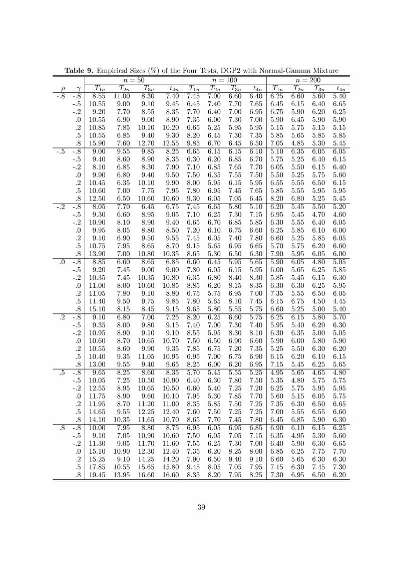
Table 9. Empirical Sizes (%) of the Four Tests, DGP2 with Normal-Gamma Mixture

n = 50 n = 100 n = 200ρ γ T1n T2n T3n t4n T1n T2n T3n t4n T1n T2n T3n t4n-.8 -.8 8.55 11.00 8.30 7.40 7.45 7.00 6.60 6.40 6.25 6.60 5.60 5.40

-.5 10.55 9.00 9.10 9.45 6.45 7.40 7.70 7.65 6.45 6.15 6.40 6.65-.2 9.20 7.70 8.55 8.35 7.70 6.40 7.00 6.95 6.75 5.90 6.20 6.25.0 10.55 6.90 9.00 8.90 7.35 6.00 7.30 7.00 5.90 6.45 5.90 5.90.2 10.85 7.85 10.10 10.20 6.65 5.25 5.95 5.95 5.15 5.75 5.15 5.15.5 10.55 6.85 9.40 9.30 8.20 6.45 7.30 7.35 5.85 5.65 5.85 5.85.8 15.90 7.60 12.70 12.55 9.85 6.70 6.45 6.50 7.05 4.85 5.30 5.45

-.5 -.8 9.00 9.55 9.85 8.25 6.65 6.15 6.15 6.10 5.10 6.35 6.05 6.05-.5 9.40 8.60 8.90 8.35 6.30 6.20 6.85 6.70 5.75 5.25 6.40 6.15-.2 8.10 6.85 8.30 7.90 7.10 6.85 7.65 7.70 6.05 5.50 6.15 6.40.0 9.90 6.80 9.40 9.50 7.50 6.35 7.55 7.50 5.50 5.25 5.75 5.60.2 10.45 6.35 10.10 9.90 8.00 5.95 6.15 5.95 6.55 5.55 6.50 6.15.5 10.60 7.00 7.75 7.95 7.80 6.95 7.45 7.65 5.85 5.55 5.95 5.95.8 12.50 6.50 10.60 10.60 9.30 6.05 7.05 6.45 8.20 6.80 5.25 5.45

-.2 -.8 8.05 7.70 6.45 6.75 7.45 6.65 5.80 5.10 6.20 5.45 5.50 5.20-.5 9.30 6.60 8.95 9.05 7.10 6.25 7.30 7.15 6.95 5.45 4.70 4.60-.2 10.90 8.10 8.90 9.40 6.65 6.70 6.85 5.85 6.30 5.55 6.40 6.05.0 9.95 8.05 8.80 8.50 7.20 6.10 6.75 6.60 6.25 5.85 6.10 6.00.2 9.10 6.90 9.50 9.55 7.45 6.05 7.40 7.80 6.60 5.25 5.85 6.05.5 10.75 7.95 8.65 8.70 9.15 5.65 6.95 6.65 5.70 5.75 6.20 6.60.8 13.90 7.00 10.80 10.35 8.65 5.30 6.50 6.30 7.90 5.95 6.05 6.00

.0 -.8 8.85 6.60 8.65 6.85 6.60 6.45 5.95 5.65 5.90 6.05 4.80 5.05-.5 9.20 7.45 9.00 9.00 7.80 6.05 6.15 5.95 6.00 5.65 6.25 5.85-.2 10.35 7.45 10.35 10.80 6.35 6.80 8.40 8.30 5.85 5.45 6.15 6.30.0 11.00 8.00 10.60 10.85 8.85 6.20 8.15 8.35 6.30 6.30 6.25 5.95.2 11.05 7.80 9.10 8.80 6.75 5.75 6.95 7.00 7.35 5.55 6.50 6.05.5 11.40 9.50 9.75 9.85 7.80 5.65 8.10 7.45 6.15 6.75 4.50 4.45.8 15.10 8.15 8.45 9.15 9.65 5.80 5.55 5.75 6.60 5.25 5.00 5.40

.2 -.8 9.10 6.80 7.00 7.25 8.20 6.25 6.60 5.75 6.25 6.15 5.80 5.70-.5 9.35 8.00 9.80 9.15 7.40 7.00 7.30 7.40 5.95 5.40 6.20 6.30-.2 10.95 8.90 9.10 9.10 8.55 5.95 8.30 8.10 6.30 6.35 5.00 5.05.0 10.60 8.70 10.65 10.70 7.50 6.50 6.90 6.60 5.90 6.00 5.80 5.90.2 10.55 8.60 9.90 9.35 7.85 6.75 7.20 7.35 5.25 5.50 6.30 6.20.5 10.40 9.35 11.05 10.95 6.95 7.00 6.75 6.90 6.15 6.20 6.10 6.15.8 13.00 9.55 9.40 9.65 8.25 6.00 6.20 6.95 7.15 5.45 6.25 5.65

.5 -.8 9.65 8.25 8.60 8.35 5.70 5.45 5.55 5.25 4.95 5.65 4.65 4.80-.5 10.05 7.25 10.50 10.90 6.40 6.30 7.80 7.50 5.35 4.80 5.75 5.75-.2 12.55 8.95 10.65 10.50 6.60 5.40 7.25 7.20 6.25 5.75 5.95 5.95.0 11.75 8.90 9.60 10.10 7.95 5.30 7.85 7.70 5.60 5.15 6.05 5.75.2 11.95 8.70 11.20 11.00 8.35 5.85 7.50 7.25 7.35 6.30 6.50 6.65.5 14.65 9.55 12.25 12.40 7.60 7.50 7.25 7.25 7.00 5.55 6.55 6.60.8 14.10 10.35 11.65 10.70 8.65 7.70 7.45 7.80 6.45 6.85 5.90 6.30

.8 -.8 10.00 7.95 8.80 8.75 6.95 6.05 6.95 6.85 6.90 6.10 6.15 6.25-.5 9.10 7.05 10.90 10.60 7.50 6.05 7.05 7.15 6.35 4.95 5.30 5.60-.2 11.30 9.05 11.70 11.60 7.55 6.25 7.30 7.00 6.40 5.90 6.30 6.65.0 15.10 10.90 12.30 12.40 7.35 6.20 8.25 8.00 6.85 6.25 7.75 7.70.2 15.25 9.10 14.25 14.20 7.90 6.50 9.40 9.10 6.60 5.65 6.30 6.30.5 17.85 10.55 15.65 15.80 9.45 8.05 7.05 7.95 7.15 6.30 7.45 7.30.8 19.45 13.95 16.60 16.60 8.35 8.20 7.95 8.25 7.30 6.95 6.50 6.20

39