Embed Size (px)
Citation preview
On-line diagnostic tool for hot stripmill
Relatório submetido à Universidade Federal de Santa Catarina
como requisito para a aprovação da disciplina:
DAS 5511: Projeto de Fim de Curso
Renato Kendy Murata
Florianópolis, Novembro de 2019


On-line diagnostic tool for hot strip mill
Renato Kendy Murata
Esta monografia foi julgada no contexto da disciplina
DAS 5511: Projeto de Fim de Curso
e aprovada na sua forma final pelo
Curso de Engenharia de Controle e Automação
Prof. Ubirajara Franco Moreno

Banca Examinadora:
Van Thang Pham
Orientador na Empresa
Prof. Ubirajara Franco Moreno
Orientador no Curso
Prof. Fabio Luis Baldissera
Responsável pela disciplina
Bernardo Schwedersky Barancelli, Avaliador
Gustavo Ardigó de Souza, Debatedor
Eduardo Marschall, Debatedor

Dedico este trabalho ao meu professor de francês Michel Abes (in memorian).
Sua vocação em ensinar e transmitir experiências me fez me encantar com um outro país.
Merci beaucoup!


Acknowledgements
This work represents the end of one cycle that started in September of 2017 with
the double degree program in France. I would like to thank everyone that make that
experience as splendid as it was.
First, I would like to thank my family, specially my father Nelson, my mother
Marineuza and my sister Cintia, to the unconditional support they gave me in my academic
life. Without their incentive, I would never have left my hometown at age 14 to dream
bigger.
I would like to thank the amazing friends that I met during this experience. They
made me feel like home even being in another country. Xiaowen, Gao, Alejandra, Rodrigo,
Sibel, Humberto, Iryna, Caio, Lucas, Carmen, Teresa, Vitor, Mônica, Isaac, Josué, Débora,
Diego, Laura and all the others. I was lucky to experienced so many great moments with
you. A special thank to Corentin, for all the support and partnership and for being the
person that I can always count with.
To my brazilian university UFSC, the french école CentraleSupelec and all the
inspiring teachers that I had the honor to learn from them, my sincere gratitude. A special
thanks to my supervisor during this program Prof. Ubirajara Franco Moreno for all the
support and disponibility.
Finally, I would like to thank all the COSMO team from ArcelorMittal Maizières
Research and specially my supervisor Van Thang Pham. You were all very kind, patient
encouraging. Thanks to you, my first professional experience was enriching and pleasant.


Resumo
A indústria siderúrgica está em constante evolução. O processo de laminação a quente,
introduzido no início do século XX, revolucionou a indústria do aço, tornando o custo de
produção de laminas de aço significativamente menores. O processo consiste em transformar
grandes barras de aço em chapas extremamente finas através de uma série de rolos. Com
o advento dos sistemas de controle, a automatização do processo de laminação a quente
deixou o processo ainda mais eficiente e rápido. Novas tecnologias trazem novos desafios,
nos processos de laminação a quente atuais, os rolos compressores chegam a uma velocidade
de 120 metros por minuto. Nessas condições, qualquer defeito ou falha no sistema deve ser
detectado o mais rápido possível, para evitar danos ou produtos defeituosos. O presente
trabalho apresenta diferentes métodos para implementar um sistema de detecção de falhas.
Primeiramente é desenvolvido um sistema para detecção de falha nos "loopers". Esse
sistema consiste em analisar os sinais adquiridos nas fábricas com diferentes métodos
de processamento de sinal, notadamente estatística descritiva, STFT e EMD, e usando
técnicas de aprendizado de máquina, classificar as informações extraídas dos sinais em dois
grupos: nominal (quando o sistema está em seu funcionamento normal) e falho (quando há
alguma falha no sistema). Esse método provou-se eficaz na detecção de falhas. Em seguida,
foi proposto um método baseado em modelo para identificação de falhas no subsistema de
"strip steering". No entanto, a implementação desse método pode ser terminada devido a
ausência de dados experimentais, necessários para a validação do modelo matemático do
sistema.
Palavras-chave: Laminação a quente. Sistema de detecção de falhas. Processamento de
sinal. Aprendizado de máquina.


Abstract
The steel industry is constantly evolving. The hot strip mill process, introduced in the
early twentieth century, reshaped the steel industry, making the cost of producing steel
sheets significantly lower. The process consists in transform thick steel slabs into thin coils
using a series of compressing rolls. With the advent of control systems, the automation of
the hot rolling process has made it even more efficient and faster. Nowadays, the rolling
speed can reach 120 meters per minute. In this condition, any default or failure must be
detected as soon as possible to avoid damages and non-quality products. This document
present different method to implement a fault detection system. First, it is developed one
fault detection system on loopers. This system analyses the signals recorded by the plant’s
data acquisition system with data processing methods, notably descriptive statistics, STFT
and EMD. By using machine learning techniques, the features extracted from the signals
are separated into two groups: the nominal (when the system has no default) and the
fault (when the system has a fault). This method proved to be efficient for fault detection
on loopers. Then, it was proposed a model-based method for fault detection on the strip
steering subsystem. Although, the method implementation wasn’t possible due to the lack
of experimental data. Those data are necessary to validate the mathematical model of the
system.
Keywords: Hot strip mill. Fault detection system. Signal processing. Machine Learning


List of Figures
Figure 1 – Finishing mill plant (From [1]) . . . . . . . . . . . . . . . . . . . . . . 22
Figure 2 – Measurement & Control department (Source: personal archive) . . . . . 24
Figure 3 – R&D Maizières campus organization (From: ArcelorMittal) . . . . . . . 24
Figure 4 – Hot strip mill (From [2]) . . . . . . . . . . . . . . . . . . . . . . . . . . 27
Figure 5 – Arcelor’s finishing mill schema (From [3]) . . . . . . . . . . . . . . . . . 27
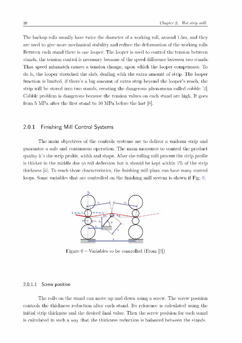
Figure 6 – Variables to be controlled (From [3]) . . . . . . . . . . . . . . . . . . . 28
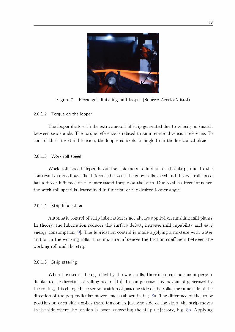
Figure 7 – Florange’s finishing mill looper (Source: ArcelorMittal) . . . . . . . . . 29
Figure 8 – Strip steering system (From [4]) . . . . . . . . . . . . . . . . . . . . . . 30
Figure 9 – Cobble fault (ThyssenKrupp Steel Europe AG) . . . . . . . . . . . . . 31
Figure 10 – Shearing-tail fault (ThyssenKrupp Steel Europe AG) . . . . . . . . . . 32
Figure 11 – Plausibility test scheme (Source: personal archive) . . . . . . . . . . . . 33
Figure 12 – Hardware redundancy scheme (Source: personal archive) . . . . . . . . 34
Figure 13 – Software redundancy scheme (Source: personal archive) . . . . . . . . . 34
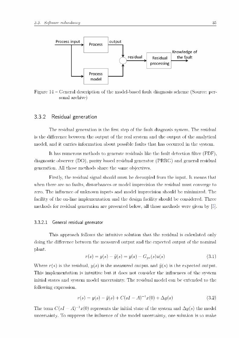
Figure 14 – General description of the model-based fault diagnosis scheme (Source:
personal archive) . . . . . . . . . . . . . . . . . . . . . . . . . . . . . . 35
Figure 15 – Signal processing structure (From [5]) . . . . . . . . . . . . . . . . . . . 40
Figure 16 – Empirical mode decomposition (Source: Towards Data Science) . . . . 43
Figure 17 – Nominal and fault signals (Source: personal archive) . . . . . . . . . . . 50
Figure 18 – Nominal and fault signals, another example (Source: personal archive) . 51
Figure 19 – Fault detection system architecture (Source: personal archive) . . . . . 52
Figure 20 – Relation between the maximum value and the median of the modeling
signals (Source: personal archive) . . . . . . . . . . . . . . . . . . . . . 52
Figure 21 – Relation between the standard deviation and the mean value of the
signals (Source: personal archive) . . . . . . . . . . . . . . . . . . . . . 53
Figure 22 – STFT results (Source: personal archive) . . . . . . . . . . . . . . . . . 54
Figure 23 – Application of EMD to nominal case (Source: personal archive) . . . . 55
Figure 24 – Application of EMD to fault case (Source: personal archive) . . . . . . 55
Figure 25 – Model validation results (Source: personal archive) . . . . . . . . . . . 57
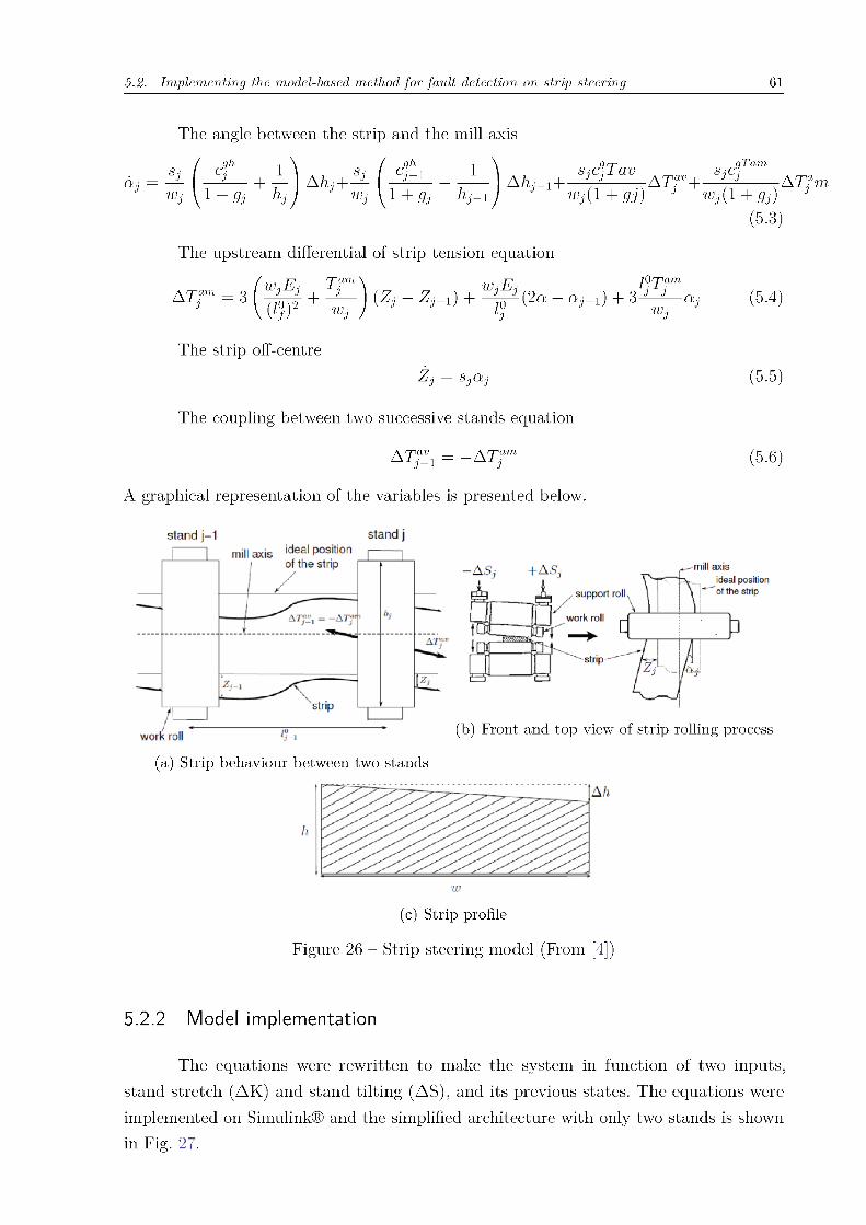
Figure 26 – Strip steering model (From [4]) . . . . . . . . . . . . . . . . . . . . . . 61
Figure 27 – Simplified Simulink model (Source: personal archive) . . . . . . . . . . 62


List of Tables
Table 1 – Numeric values of model validation . . . . . . . . . . . . . . . . . . . . . 58
Table 2 – The most efficient techniques for fault detection on loopers . . . . . . . 58
Table 3 – Strip steering parameters . . . . . . . . . . . . . . . . . . . . . . . . . . 60


List of abbreviations and acronyms
SSU: Shared Services Unit
MC: Measurement & Control department
COSMO: Control , Simulation and Models
HAGC: Hydraulic automation gauge control
HSM: Hot strip mill
FD: Fault detection
FDI: Fault detection and isolation
FDIA: Fault detection and isolation and Analysis
FDF: Fault detection filter
DO: Diagnostic observer
PRRG: Parity based residual generator
LCF: Left coprime factor
SDFA: Set of disturbances that causes false alarms
FDR: Fault detection rate
FFT: Fast Fourier transform
STFT: Short time Fourier transform
EMD: Empirical mode decomposition
SVM: Support vector machine


Contents
1 INTRODUCTION . . . . . . . . . . . . . . . . . . . . . . . . . . . . 21
1.1 Motivation of the project . . . . . . . . . . . . . . . . . . . . . . . . . 21
1.1.1 ArcelorMittal . . . . . . . . . . . . . . . . . . . . . . . . . . . . . . . . . 22
1.1.1.1 ArcelorMittal Global R&D . . . . . . . . . . . . . . . . . . . . . . . . . . . 23
1.1.1.2 ArcelorMittal Maizières Research SA . . . . . . . . . . . . . . . . . . . . . . 23
1.1.1.3 Measurement & Control department . . . . . . . . . . . . . . . . . . . . . . 23
1.1.1.4 COSMO team . . . . . . . . . . . . . . . . . . . . . . . . . . . . . . . . . 24
1.1.2 Project objectives . . . . . . . . . . . . . . . . . . . . . . . . . . . . . . . 25
1.2 Structure of the document . . . . . . . . . . . . . . . . . . . . . . . . 25
2 HOT STRIP MILL . . . . . . . . . . . . . . . . . . . . . . . . . . . 27
2.0.1 Finishing Mill Control Systems . . . . . . . . . . . . . . . . . . . . . . . . 28
2.0.1.1 Screw position . . . . . . . . . . . . . . . . . . . . . . . . . . . . . . . . . 28
2.0.1.2 Torque on the looper . . . . . . . . . . . . . . . . . . . . . . . . . . . . . . 29
2.0.1.3 Work roll speed . . . . . . . . . . . . . . . . . . . . . . . . . . . . . . . . 29
2.0.1.4 Strip lubrication . . . . . . . . . . . . . . . . . . . . . . . . . . . . . . . . 29
2.0.1.5 Strip steering . . . . . . . . . . . . . . . . . . . . . . . . . . . . . . . . . 29
2.1 Possible faults on Hot Strip Mill plant . . . . . . . . . . . . . . . . . 30
2.1.1 Faults on actuators . . . . . . . . . . . . . . . . . . . . . . . . . . . . . . 30
2.1.2 Cobbles . . . . . . . . . . . . . . . . . . . . . . . . . . . . . . . . . . . . 31
2.1.3 Shearing-tails . . . . . . . . . . . . . . . . . . . . . . . . . . . . . . . . . 31
3 FAULT DETECTION THEORY . . . . . . . . . . . . . . . . . . . . 33
3.1 Plausibility test . . . . . . . . . . . . . . . . . . . . . . . . . . . . . . . 33
3.2 Hardware redundancy . . . . . . . . . . . . . . . . . . . . . . . . . . . 33
3.3 Software redundancy . . . . . . . . . . . . . . . . . . . . . . . . . . . . 34
3.3.1 Analytical model-based fault detection . . . . . . . . . . . . . . . . . . . . 34
3.3.2 Residual generation . . . . . . . . . . . . . . . . . . . . . . . . . . . . . . 35
3.3.2.1 General residual generator . . . . . . . . . . . . . . . . . . . . . . . . . . . 35
3.3.2.2 Optimal fault detection filter . . . . . . . . . . . . . . . . . . . . . . . . . . 36
3.3.2.3 Parity space method . . . . . . . . . . . . . . . . . . . . . . . . . . . . . . 37
3.3.3 Fault detectability, isolability and identifiability . . . . . . . . . . . . . . . 37
3.3.4 Structural fault detectability . . . . . . . . . . . . . . . . . . . . . . . . . 37
3.3.5 Structural fault isolability . . . . . . . . . . . . . . . . . . . . . . . . . . . 38
3.3.6 Structural fault identifiability . . . . . . . . . . . . . . . . . . . . . . . . . 39
3.4 Signal processing . . . . . . . . . . . . . . . . . . . . . . . . . . . . . . 39

3.4.1 Symptom generation . . . . . . . . . . . . . . . . . . . . . . . . . . . . . 40
3.4.1.1 Descriptive statistics . . . . . . . . . . . . . . . . . . . . . . . . . . . . . . 40
3.4.1.2 Fast Fourier transform (FFT) . . . . . . . . . . . . . . . . . . . . . . . . . . 41
3.4.1.3 Short time Fourier transform (STFT) . . . . . . . . . . . . . . . . . . . . . . 42
3.4.1.4 Empirical mode decomposition (EMD) . . . . . . . . . . . . . . . . . . . . . 42
4 DEVELOPMENT OF AN APPLICATION FOR FAULT DETECTION 45
4.1 The proposed signal processing method for fault detection . . . . . 45
4.1.1 Data reading . . . . . . . . . . . . . . . . . . . . . . . . . . . . . . . . . 45
4.1.1.1 Pre-processing . . . . . . . . . . . . . . . . . . . . . . . . . . . . . . . . . 45
4.1.2 Data processing . . . . . . . . . . . . . . . . . . . . . . . . . . . . . . . . 46
4.1.3 Data classification . . . . . . . . . . . . . . . . . . . . . . . . . . . . . . 46
4.1.3.1 Support Vector Machine (SVM) . . . . . . . . . . . . . . . . . . . . . . . . 47
4.1.3.2 Classification Tree . . . . . . . . . . . . . . . . . . . . . . . . . . . . . . . 48
4.1.3.3 Cross-Correlation . . . . . . . . . . . . . . . . . . . . . . . . . . . . . . . . 48
4.2 Implementing the signal processing method for fault detection on
loopers . . . . . . . . . . . . . . . . . . . . . . . . . . . . . . . . . . . . 49
4.3 Data selection . . . . . . . . . . . . . . . . . . . . . . . . . . . . . . . . 50
4.3.1 Pre-processing . . . . . . . . . . . . . . . . . . . . . . . . . . . . . . . . 51
4.4 Data processing . . . . . . . . . . . . . . . . . . . . . . . . . . . . . . . 51
4.4.1 Descriptive statistics . . . . . . . . . . . . . . . . . . . . . . . . . . . . . 52
4.4.2 Short-time Fourier Transform (STFT) . . . . . . . . . . . . . . . . . . . . 53
4.4.3 Empirical Mode Decomposition (EMD) . . . . . . . . . . . . . . . . . . . 54
4.5 Data Classification . . . . . . . . . . . . . . . . . . . . . . . . . . . . . 56
4.5.1 Classification Tree . . . . . . . . . . . . . . . . . . . . . . . . . . . . . . 56
4.5.2 Support vector machine . . . . . . . . . . . . . . . . . . . . . . . . . . . 56
4.5.3 Cross Correlation . . . . . . . . . . . . . . . . . . . . . . . . . . . . . . . 56
4.6 Implementation results . . . . . . . . . . . . . . . . . . . . . . . . . . 56
4.7 Experimental results and validation . . . . . . . . . . . . . . . . . . . 57
5 MODEL-BASED FAULT DETECTION ON STRIP STEERING . . . 59
5.1 The proposed model-based method for fault detection . . . . . . . . 59
5.2 Implementing the model-based method for fault detection on strip
steering . . . . . . . . . . . . . . . . . . . . . . . . . . . . . . . . . . . 59
5.2.1 Mathematical equations . . . . . . . . . . . . . . . . . . . . . . . . . . . 60
5.2.2 Model implementation . . . . . . . . . . . . . . . . . . . . . . . . . . . . 61
5.2.2.1 Model Validation . . . . . . . . . . . . . . . . . . . . . . . . . . . . . . . . 62
6 SUMMARY AND FUTURE WORK . . . . . . . . . . . . . . . . . . 63
6.1 Summary . . . . . . . . . . . . . . . . . . . . . . . . . . . . . . . . . . 63

6.2 Future work . . . . . . . . . . . . . . . . . . . . . . . . . . . . . . . . . 63
BIBLIOGRAPHY . . . . . . . . . . . . . . . . . . . . . . . . . . . . 65


21
1 Introduction
The 20th century lead the world to a new era with a chain of events that had a
great impact in our society. In the 1960s a big quantity of theories was developed and had
a great contribution in controls design. Nowadays, with the control theory consolidated
in the industry and the automation degree of process continuously growing, there is an
increasing demand for higher system perform and product quality. To increase the perform
of the system and the product quality, it is required more system safety and reliability.
One way to have a safer and more reliable process is by building a fault diagnosis
system. Those diagnosis systems are built to detect faults that a simply process monitoring
system would not detect, like sensor faults and actuator faults. A fault diagnosis system
can be developed in many ways, the main methods are the hardware redundancy schemes,
plausibility test, software redundancy schemes and by signal processing. During this project,
it was developed a fault detection system using the software-redundancy test and the
signal processing.
The fault diagnosis system aims to detect fault in a hot strip mill plant. The plant
transforms thick stabs of steel into thin coils. It is an expensive process because of the
wear of actuators, that must be often changed, and due to the size of the system, any
fault can be dangerous for the operators that are working next to it. The rolling process,
Fig. 1, is an important method in the metal industry. The product must have very precise
dimension, in the micro meter range.
1.1 Motivation of the project
The hot strip mill process consists hundred of sensors and actuators to ensure the
process operation. The rolling speed can reach up to 120m/min. At that speed, any fault
can have serious damages on the plant, and also have an influence on the product quality.
Even with the most advanced sensors and actuators, and making a regular maintenance of
the components, the process is not immune to faults.
According to a study made by SCHAFFLER on the ThyssenKrupp Steel Europe
AG’s facilities in Germany shown that one repair on the work rolls of the hot strip mil
plant costs around e21000 euros. In one year, this problem happened 5 times, totalizing
an extra charge of e105000 euros per year due to unplanned stoppage. Also, 5 unplanned
roller replacement of 7 minutes each costs e35000 euros. So, in this case, the unpredictable
faults in one hot strip mill during year costs around e140000 euros.


1.1. Motivation of the project 23
steep products. The steel is produced all over the world. Europe is the biggest producer
corresponding to 47% of the steel production, the Americas produces 38% and the other
regions 18%. ArcelorMittal’s products are organised according to region, each region is
specialized in a set of products.
1.1.1.1 ArcelorMittal Global R&D
The research and development have a big importance in the ArcelorMittal’s strate-
gies. The main goal of the R&D sector is to realise ArcelorMittal’s ambitions in technological
innovation, and ensuring future growth with focus on sustainability. The company has
10 research centers distributed in North America, Europe and South America, with more
than 1400 researchers. The R&D is highly business oriented, it is focused on seven key
areas: automotive, packaging, construction, general industry, energy market, long prod-
ucts and special plates. Those centers ensures a shorter time to market and improved
competitiveness.
1.1.1.2 ArcelorMittal Maizières Research SA
The project took place in Maizières’s campus. The Maizière campus is the biggest
global R&D campus. With 24 hectares and 45.000 m2 of laboratories, the Maizière center
has 570 permanent employees and receives around 100 interns per year. The campus hosts
four different research centres: Maizière Process, Maizière Products, Maizières Mining
and Shared Services Unit (SSU). Those centres are specialized in automotive products,
packaging, process development and mining processing.
1.1.1.3 Measurement & Control department
The internship took place in the Measurement & Control Department (MC). The
department is part of the Maizière Process center. The MC department is composed of three
teams: Advanced Process Instrumentation and product non destructive evaluation; Surface
Properties, Image & Data processing; and COntrol, Simulation and MOdels (COSMO).
The main mission of those teams is to bring relevant solutions for the different process
involved in the productive chain of the steel products. Those solutions are searched in the
fields of process control, instrumentation and product inspection and evaluation.


1.2. Structure of the document 25
1.1.2 Project objectives
The objective of the internship is to carry out a feasibility of different fault detection
methods for hot strip mill process. The idea is to take advantage of the huge amount of data
that is recorded with the hot strip mill plant data acquisition system to perform an on-line
fault detection of the system. The methods can be model-based methods, data-oriented
method as well as knowledge-based methods. To develop such a system, the following
tasks are expected:
• Bibliography revision of preview works with the same subject
• Try different methods on real industrial historic data
• Develop a toolbox for facilitating further usage
• Establish a final report to capitalize the study
1.2 Structure of the document
This document is divided into six chapters. In chapter 1, the motivation of the
project and its main objectives is given. The enterprise organization and the details about
the place where the internship took place is also presented in chapter 1. Chapter 2 presents
the hot strip mill system and its components. It also contains the possible faults on hot
strip mill plant that were found in the bibliography revisions. In chapter 3 the fault
detection theory is presented, this chapters gives an overview on two different methods:
signal processing and model-based. Chapter 4 proposed a signal processing method for
fault detection, the method is applied for the looper subsystem and its results are analyzed.
In chapter 5 a model based method for fault detection on strip steering subsystem is
presented. Chapter 6 summarizes the main results of this project and presents and outlook
for future work.


36 Chapter 3. Fault detection theory
one closed loop structure as one output observer with the following structure.
y(s) = Gyu(s)u(s) + L(s)(y(s) − y(s)) (3.3)
Rewriting the previous expression in the state space model, we must define the L matrix
ensuring A − LC stable and with the desired dynamic. It was proven on [5] that the
residual of the closed loop structure presented can be expressed by the formula
r(s) = Mu(s)y(s) − Nu(s)u(s) (3.4)
where the transfer matrices Mu and Nu are the left coprime factor (LCF) of the Gyu(s)
function and can be obtained with the following expression.
Mu = (A − LC, −L, C, I), Nu = (A − LC, B − LD, C, D) (3.5)
This method is easy to design but it requires complex computation, which can difficult
the on-line realization. Choosing L is also a problem, and it was the subject of various
residual generation approached in the last three decades.
3.3.2.2 Optimal fault detection filter
In this section the optimal tuning of the fault detection filter is presented. This
regulation minimizes the set of disturbances that causes false alarms (SDFA) in function
of a given fault detection rate (FDR). Having the following state space system
x(t) = Ax(t) + Bu(t) + Edd(t) + Eff(t)
y(t) = Cx(t) + Du(t) + Fdd(t) + Fff(t)(3.6)
we must generate residuals using one FDF of the form
xa = Axa(t) + Bu(t) + L(y(t) − ya(t))
ya(t) = Cxa(t) + Du(t)
r(t) = V (y(t) − ya(t))
(3.7)
The optimal L and V gains can be obtained using the following equations
Lopt = (EfF ′
f + YfC ′)(FfF ′
f )−1
Vopt = (FfF ′
f )1
2
(3.8)
with Yf being the solution of the Riccati equation
AYf + YfA′ + EfE ′
f − (EfF ′
f + YfC ′)(FfF ′
f )−1(FfE ′
f + CYf ) = 0 (3.9)
This function can be numerically solved using the function care from MATLAB®.
A′
eXEe + E ′
eXAe − (E ′
eXBe + Se)R−1e (B′
eXEe + S ′
e) + Qe = 0
Ae = A′ Be = C ′ Q = EfE ′
f
R = FfF ′
f S = EfF ′
f E = Isize(A)

3.3. Software redundancy 37
3.3.2.3 Parity space method
As shown on [11] parity equations are a straightforward method for fault detection.
Developed on the 80’s, this method is simple do construct and implement, it’s a method
indicated to detect additive faults and it has similar results of more complicated methods
presented in previous sections.
First we need a model Gm(s) of the process Gp(s). The residual can be calculated
by the following formula
r(s) = [Gp(s) − Gm(s)]u(s) + Gp(s)fu(s) + fy(s) (3.10)
If the model is accurate, Gm(s) = Gp(s), so the first part of the equation is equal
to zero. The residual value is only different to zero if the additive input fault fu(s) 6= 0
and the additive output fault fy(s) 6= 0
3.3.3 Fault detectability, isolability and identifiability
A model-based fault detection cannot detect all the faults of the system, there are
some conditions have to be validated to detect, isolate and identify a fault, in a FDI point
of view. The theorems used in this section were obtained on [5].
3.3.4 Structural fault detectability
A fault is detectable if its occurrence, independent of its size and type, would cause
a change in the nominal behaviour of the system output. To define in which conditions a
fault can be detectable, we recall the following theorem
Theorem 1. Given the system
x = (A + ∆Af )x + (B + ∆Bf )u + Eff
y = (C + ∆Cf )x + (D + ∆Df )u + Fff
Where f is the additive fault vector and ∆Af , ∆Cf , ∆Bf and ∆Df are the multiplicative
faults given by
∆Af =lA∑
i=1
AiΘAi, ∆Bf =
lB∑
i=1
BiΘBi
∆Cf =
ICf∑
i=1
CiΘCi, ∆Df =
lD∑
i=1
DiΘDi
An additive fault fi is detectable if and only if
C(sI − A)−1Efi+ Ffi
6= 0

38 Chapter 3. Fault detection theory
with Efi, Ffi
denoting the i-th column of matrices EfFf respectively, a multiplicative fault
ΩAiis detectable if and only if
C(sI − A)−1Ai(sI − A)−1B 6= 0
a multiplicative fault ΘBiis detectable if and only if
C(sI − A)−1Bi 6= 0
A multiplicative fault ΘCiis detectable if and only if
Ci(sI − A)−1B 6= 0
A multiplicative fault ΘCiis detectable if and only if
Di 6= 0
From Theorem 1 , we can conclude that an additive fault is detectable if the
transfer function between the fault and the system output is not zero. A multiplicative
fault ΘDiis always detectable and the detectability of fault ΘBi
can be interpreted as
input controllability and the ΘCithe observability. The multiplicative fault ΘAi
can change
the system dynamics.
It is evident that detecting additive faults can be realized independent of the system
input, and multiplicative faults is possible do be detected if the input signal is not zero.
This conclusion explain why sensor faults are usually modelled as additive faults and
actuators faults as multiplicative faults.
3.3.5 Structural fault isolability
In this context, it is considered a system with the influence of two faults, unknown
inputs are not taken into account. We take two faults, ξi ,ξj ,i 6= j are possible to isolate if
the changes in the system output caused by these two faults are distinguishable. To check
the conditions of fault isolability, we now use a the following corollary.
Corollary 1. Given the system used in theorem 1, then ξ with fault transfer matrix
Gξ(s) = [Gξ1(s)...Gξl(s)]
Is structurally isolable if and only if
rank(Gξ(s)) =l∑
i=1
rank(Gξi(s))

3.4. Signal processing 39
For additive faults for example, this result means that the faults are isolable only
if the number of faults is not larger than the number of sensors. With multiplicative fault,
the fault transfer matrix is different so it may demand more sensors. It is possible to
archive fault isolation even if this corollary is not satisfied by removing some assumption
as having previous knowledge of faults, or assuming that a simultaneous occurrence of
faults is impossible.
3.3.6 Structural fault identifiability
Fault identifiability characterizes the mapping from the system output to the faults
under consideration. If this mapping is unique, then the faults are identifiable. The formal
definition is presented below.
Definition 1. Given the system used in theorem 1, then ξ with fault transfer matrix
Gξ(s) = [Gξ1(s)...Gξl(s)]
the fault vector is called structurally identifiable if Gξ(s) is invertible and its inverse is
stable and casual.
It is a necessary condition the fault transfer function be invertible and stable,
otherwise the fault identifiability structure will be equivalent to the fault isolability
scheme.
3.4 Signal processing
The basic architecture for fault detection using signal processing is shown is Fig.
15. In this case we consider that the system’s outputs carry information about faults. The
symptom generation will catch all relevant information about the possible faults present
in the signal. Typical faults usually have influence on time domain functions, like mean
values, limit values, standard deviation or frequency domain functions like spectral power
densities, etc. The main drawback for signal processing methods is its inefficiency with
dynamic systems, where the input signals changes very often. In other hand, this method
is easy to implement and it does not requires much information about the system.


3.4. Signal processing 41
The standard deviation calculates the amount of dispersion of a list of values
and can be calculated by the following formula
s =
√√√√ 1
N − 1
N∑
i=1
(xi − x)2
where x is the arithmetic mean and N is the amount of values of the list.
• Variance
The variance is the expectation of the squared deviation of a random variable
from its mean [12].
V ar(X) = E[(X − µ)2
]
• Range
The range of a set of data is the difference between the largest and smallest values [12].
• Limit values
The maximum and the minimum value of a list of values.
3.4.1.2 Fast Fourier transform (FFT)
The fast Fourier transform is the discrete version of the Fourier transform. The
Fourier transform convert a signal in time domain into the frequency domain. The Fourier
transform plays a very important roll in signal processing because it represents a signal as
sum of complex sinusoids. Having a signal described as a sum of complex sinusoids, it is
possible to make a spectral analysis of the signal.
The spectral analysis is a important component of signal processing. For example,
it can give information on the wear of mechanical components of one system by monitoring
its vibration, and it can also identifies cyclic behaviours hidden in a signal.
The fast Fourier transform (FFT) is one algorithm to perform a Fourier transform
of a dataset. The FFT can be calculated by the following formula [13] with y(t) being the
signal.
Y (k) =N∑
t=1
y(t)e−i2πkt/N k = 0, . . . , N − 1,
The fast Fourier transform is recommended for stationary signals because it applies the
formula over the entire signal.

42 Chapter 3. Fault detection theory
3.4.1.3 Short time Fourier transform (STFT)
The short time Fourier transform is another method based on the Fourier transform.
This method instead of applying the Fourier transform in the whole signal, as the FFT
does, it splits, over the time, the entire signal into smaller parts. So the FFT is applied for
each part of the signal.
This is a solution for spectrum analysis when it comes to non-stationary signals.
When we take the whole signal and divide it into smaller parts, each part is considered
to be stationary, so it makes sense to apply the FFT over the smaller part. As a result,
we can extract information about the evolution of the most important frequencies of the
signal over the time. The STFT is considered to be a time-frequency method because it
carries information about both variables.
The discrete STFT can be calculated with the following formula [2]
X(m, ω) =∞∑
n=−∞
x[n]w[n − m]e−jωn
where X(m, ω) are the Fourier coefficients depending on time index m and frequency ω, x
is the signal and w is the window function.
3.4.1.4 Empirical mode decomposition (EMD)
The empirical mode decomposition is another time-frequency method for signal
processing of non-stationary signals. It’s an empirical method, different from STFT and
FFT, and it decomposes the signal into intrinsic mode functions (IMF).
IMFs represents specific oscillations of the original signal [2]. This method was
developed by NASA’s engineer Norden E. Huang on 1988. According to its definition, one
IMF should satisfy two conditions “... the number of extrema and the number of zero
crossings must either equal or differ at most by one” and “the mean value of the envelope
defined by the local maxima and the envelope defined by the local minima is zero” [14]
The EMD method can be perform by the following algorithm [15]
1. Initialize: r1 = x (t) , and i = 1
2. Extract the ith IMF
a) Initialize: hi(k−1) = ri, k = 1
b) Extract the local extrema and the minima of hi(k−1)
c) Cubic spline interpolation of local extrema from upper and lower envelopes of
hi(k−1)

3.4. Signal processing 43
d) Calculate the mean mi(k−1) of the upper and lower envelopes of hi(k−1)
e) Let hik = hi(k−1) − mi(k−1)
f) If hik is an IMF then set IMFi = hik, else go to step (b) with k = k + 1
3. Define ri+1 = ri − IMFi
4. If ri+1 still has least 2 extrema then go to step (2) else decomposition process is
finished and ri+1 is the residue of the signal
Figure 16 – Empirical mode decomposition (Source: Towards Data Science)


45
4 Development of an application for fault de-
tection
In this chapter, it is proposed a signal processing method for fault detection.
The method combine signal processing techniques with machine learning algorithms. Its
implementation for fault detection on loopers is shown in section 4.2. Then the results of
the validation are discussed.
4.1 The proposed signal processing method for fault detection
The hot strip mill plant, as presented on section 2, has a lot of sensor and actuators,
the signals transmitted and emitted by those components contains information about
the system state. On ArcelorMittal’s steel mills, those signals are stored using the IBA®
measurement system. The main idea is to take advantage of the huge amount of signals
that were record to build a signal processing fault detection system.
The proposal is to build a fault detection system that can be divided into three
parts:
1. Data reading
2. Data processing
3. Data classification
4.1.1 Data reading
This is the most simple task of the proposed method. The system will be developed
on MATLAB® platform, and the signals are recorded using the IBA® measurement system.
As the acquisition system is already complete and working, it’s just necessary to convert
the IBA® files into MATLAB® ".dat" format.
4.1.1.1 Pre-processing
The hot strip mill plant record hundreds of signals not all of them are useful or
contains information about the state of the system. In this part, the useful signals for fault
detection are selected and the useless part of those signals are removed. Some signals like
46 Chapter 4. Development of an application for fault detection
the input of the motor that controls the looper for example, when the looper is not used,
the signal is zero and it doesn’t have any useful information.
The pre-processing take care of the useless signals. It is an important task because
the signal processing requires a considerable computational effort, like the Fourier or
Wavelet transforms. When the data is clean, less computational effort is required so the
system is more efficient and faster.
4.1.2 Data processing
The data processing is the most important part of the method. It’s necessary to
use the right methods for features extraction, so the data classification will have more
success and the fault detection system will be more precise and accurate.
For features extraction, the proposed technique is to try different methods studied
on section 3.4.1:
• Descriptive statistics
• Short time Fourier transform
• Empirical mode decomposition
Those three methods were chosen because they have completely different characteristics.
Descriptive statistics like the mean, variance and standard deviation are very easy to
calculate and can give a lot of information about the signal. The STFT is a theoretical tool
based on the Fourier transform and it’s possible to analyse the evolution of the frequencies
over the time of one signal. The EMD is different from both of them, it’s a empirical
method and can be useful when the signal is too complex or non-stationary.
4.1.3 Data classification
The features extracted by the methods presented in the previous section need to be
classified into fault or nominal data. As there’s an important amount of signals recorded,
it was chosen two machine-learning methods: support vector machine and classification
tree. The cross-correlation method is used to classify the EMD results, following the signal
processing method presented on [5]. In this section, a basic theory about those classification
method is given.

4.1. The proposed signal processing method for fault detection 47
4.1.3.1 Support Vector Machine (SVM)
The support vector machine is a learning model that can be used for data classi-
fication. In our case, we have to give the data from the feature extraction labeled into
two groups: the nominal and the fault data. The SVM algorithm will create an optimal
hyperplane to separate the both data. The optimal hyperplane created to separate the
training data can be used to classify new data. So, by using a big amount of labeled and
recorded data, it is possible to train a SVM model to classify the new data.
The mathematical basis to develop a system with such characteristics is given
by [16].
The data needed for training is given in the following form
(y1, x1)...(yn, xn) x ∈ Rn, y ∈ −1, +1 (4.1)
The hyper plane is defined as
H(ω, b) = ∀x|ωT x + b = 0 (4.2)
where b is the parameter needed to calculate the normal distance of the hyperplane to the
origin and ω is the normal vector to the hyperplane. The prameters in Equation 4.2 are
scalable, meaning that
H(ω, b) = ∀x|cωT x + cb = 0 (4.3)
with c ∈ R and c 6= 0 lead to the same hyperplane as Equation 4.2 The optimal hyperplane
has to fulfil the condition below
minxi|ωT xi|
!= 1 (4.4)
The euclidean distance of a point xi to the hyper plane is
d(H; x) =|ωT xi + b|
||ω||(4.5)
The support vectors are the the data points xi closest to the hyperplane. The distance
between the data points and the hyperplane is called margin, must reach a maximum. The
distance can be calculated by the following formula
ζ(H) = minxid(H; xi) =
1
||ω||[minxi
|ωT xi + b|] =1
||ω||(4.6)
The maximum ζ is reached when ||ω|| is minimized. The optimization problem below must
be solved
Θ(ω) = argminω,b[1
2||ω||2] (4.7)
The following constraint must be assumed to not violate the condition 4.4
yi((ωT xi) + b) ≥ 1, i = 1, ...n (4.8)

48 Chapter 4. Development of an application for fault detection
The optimization problem with constraints can be solved using the Lagrange’s method of
multipliers
ω =n∑
i=1
αiyixi (4.9)
for ω, with αi being the Lagrange multipliers
b = −1
2ω[xr + xs] (4.10)
for b, where the indiced r and s indicate the support vectors
αr, αs > 0, yr = 1, ys = −1 (4.11)
finally, the optimal hyperplane is
f(x) = sign(ωT x + b) (4.12)
4.1.3.2 Classification Tree
The classification tree is a very simple and efficient tool that can be used in data
classification. The classification tree can be seen as a binary tree. Each root node of the
tree represents one input and the leaf nodes represents the output of the tree. The C4.5
algorithm [17] is one solution to implement a classification tree.
• Check for base cases
1. For each attribute a
a) Find the feature that best divides the training data such as information
gain from splitting on a
2. Let a best be the attribute with the highest normalized information gain
a) Create a decision node node that splits on a_best
• Recurse on the sub-lists obtained by splitting on a best and add those nodes as
children of node
4.1.3.3 Cross-Correlation
The cross-correlation function on signal processing tells the similarity of two given
signals. The function is defined by the following expression
Cx1x2(σ) = lim
Tf →∞
1
Tf
∫ Tf /2
−T f/2x1(t)x2(t + σ)dt (4.13)
The method proposed by [5] for fault detection using cross-correlation is to calculate the
auto-correlation between the IMF’s obtained with the EMD method, discussed on section

4.2. Implementing the signal processing method for fault detection on loopers 49
3.4.1.4, in the feature extraction part. The auto-correlation is the cross-correlation function
applied to the same signal divided into two parts. Having the results of the auto-correlation,
the magnitude and the position where the correlation was more important is saved. Those
values gives information about the symmetry of the signal. If the highest magnitude of the
correlation is when the position is close to zero, it means that the IMF is highly symmetric.
The method proposes to use those symmetric information to define thresholds to classify
the data into two states.
In our case, instead of define thresholds to classify the data, we propose to use the
machine learning methods, SVM or classification tree. So, as training data, instead of the
features extracted by the data processing part, the machine learning methods used the
information about similarity of the IMFs obtained with the cross-correlation function.
4.2 Implementing the signal processing method for fault detection
on loopers
The signal processing method for fault detection on loopers was implemented using
the recorded data from 2016 to 2018 from Florange factory. The hot strip mill plant has
an iba® measurement system. This system acquires hundreds of signals during the whole
milling process. The signal-based fault detection model was made to identify fault on
loopers. In the looper subsystem, 18 signals are recorded by the iba® measurement system.
Some of the most important signals recorded are:
• Angular position measure/reference
• Speed measure/reference
• Torque measure/reference
• Servomotor reference
• Pression on hydraulic cylinder
There are 2297 files recorded in total. It’s known that 1827 files represent the
nominal behaviour of the system. The other 470 files were recorded when the system was
on its faulty state. It’s not defined the exact fault presented in the system, or how many
faults can be found on the faulty files. It is just known that those files don’t represents
the nominal behaviour of the system.


56 Chapter 4. Development of an application for fault detection
4.5 Data Classification
After the feature extractions, the next step is the classification. To implement
different classification methods, it was used the MATLAB® Classification Learner app.
The basic statistical features were classified using SVM and classification tree. The STFT
results were sorted using classification three. The EMD results were first classified using
cross-correlation and then with SVM.
4.5.1 Classification Tree
The classification tree was applied to the basic statistics features and to the STFT
data. For the basic statistics features, each feature (mean, median, maximum value,
minimum value, standard deviation and variation) is an input to the classification tree, as
result, it indicates the state of the system. The STFT data were also used as input in the
classification tree. The results are presented in the next section.
4.5.2 Support vector machine
The SVM was used to classify the features extracted by the data processing methods
into the two system states. The classification tree has the same input as the SVM. So our
objective here is to compare which classification method is more efficient to identify faults
in the signal that is being used.
4.5.3 Cross Correlation
The features extracted using the EMD method were auto-correlated. From each
result of the autocorrelation it was extracted the maximum point of correlation. If the signal
is symmetric for example, the highest autocorrelation would be in 0. That information
was used as input for the support vector machine training.
4.6 Implementation results
In total, we had 2297 files recorded. Around 80% represented the system on its
nominal behaviour and the other 20% the system on its fault state. For modeling, 60% of
each type of file were used. So the other 40% were reserved to do the validation. The files
were chosen randomly, to minimize the influence of the period when the file was recorded.


58 Chapter 4. Development of an application for fault detection
Table 1 – Numeric values of model validation
Model False positive rate True positive rateDescriptive statistics - Tree 3.7% 99.0%Descriptive statistics - SVM 4.2% 99.7%STFT - Tree 52.2% 98.2%EMD-CC-SVM 70.7% 97.8%
It’s clear that for fault detection, the best results are the combination between
basic statistics and a given classification method. The classification tree has a singly better
fault positive rate, and a worst true positive rate comparing to the SVM. Considering that
this is a fault detection system, it’s better to have a false alarm instead of doesn’t identify
one fault. So, the basic statistics features combined with SVM classifier is the best choice.
The other two model has shown worst results. It shows that for fault detection on
loopers, time-frequency analysis aren’t good methods for features extraction. However,
those methods should be considered when it comes to fault identification, but to perform
a fault identification it is required more information about the fault.
Another reason that should be considered to understand why the more complex
methods didn’t give good results is that is not known how many type of faults were present
on the files. Both features extraction systems, STFT and EMD, had a big false alarm rate.
It means that with the system is too sensible to identify faults.
So, the best signal processing method for fault identification on loopers are the
descriptive statistics combined with support vector machine or classification tree.
Table 2 – The most efficient techniques for fault detection on loopers
Model False positive rate True positive rateDescriptive statistics - Tree 3.7% 99.0%Descriptive statistics - SVM 4.2% 99.7%

59
5 Model-based fault detection on strip steer-
ing
After speaks with specialists from the factories. It was noticed that the loopers
aren’t a big problem on the hot strip mill plant. Those faults are not the most frequent
and it’s not a reason for a big concern from the operators.
The most problematic part of the hot rolling process is the strip tracking. Usually
the strip gets out of its desired path, this deviation can cause serious faults like the ‘cobble’
which also very dangerous for the operators.
This chapter proposes a model-based fault identification system on strip steering.
5.1 The proposed model-based method for fault detection
Model-based methods are much more complex to develop than signal based ones. It
requires an accurate model of the system and the fault detection, isolation and identification
is much more complex. In other hand, those models are usually better on fault identification
and much more flexible to changes on the plant.
As seen in previous sections, there’s many ways to build a model-based fault
detection system. The proposed solution in presented below.
1. Build a dynamic model
• Validate the model
2. Study the faults on the system and build model for the faults
3. Linearize the system
4. Apply the methods presented on section 3.3.2
5. Validate the fault identification system with real data
5.2 Implementing the model-based method for fault detection on
strip steering
The first step to implement the proposed solution is to build a dynamic model for
the system. When the strip steering control, see 2.0.1.5, was implemented, one dynamic

60 Chapter 5. Model-based fault detection on strip steering
model was developed. The idea was to use the same model for fault detection on the strip
path.
5.2.1 Mathematical equations
Those equations were developed by ArcelorMittal’s engineers when the strip steering
control was developed [18]. The non-linear equations shows the relation between the
parameters presented on table 3.
Table 3 – Strip steering parameters
Parameter Description∆Pj Differential rolling force∆hj Strip thickness profile∆Sj Stand tilting∆Kj Differential stand stretch∆T am
j Upstream differential of strip tension
∆T avj Downstream differential of strip tension
Zj Strip off-centreEj Young’s modulesj Work roll speedbj Work roll lengthl0j Inter-stand length
lvj The screw inter-axis length
T avj The front strip tension
T amv The back strip tension
hj Strip thicknesswj Strip width
cfhj , c
fTam
j , cfTav
j cghj Constants to represent the gradient of the strip parameters
cgTam
j , cgTav
j , Khj , K
fj , K l
j, Pj, gj Constants to represent the gradient of the strip parameters
The main equations governing the system are presented below.
The differential rolling force equation
∆Pj = cfhj−1∆hj−1 + cT am
j ∆T amj + c
fT avj ∆T av
j (5.1)
The exit stand wedge equation
∆hj =
wj
(lv)2jK
hj
+6wj
b2jK
fj
(∆Pj − 2Pj) Zj +
∆Pj
K lj
+wj
lvj
∆Sj −wj
lvj (Kh
j )2Pj (5.2)


63
6 Summary and future work
6.1 Summary
The project presents two different methods for fault detection on hot strip mill
plants: signal processing and model-based. The signal processing method was used for fault
detection on looper by analysing the servo-motor signal. The signals were firstly analysed
through short time Fourier transform, empirical mode decomposition and basic descriptive
statistics. Then the data was classified using machine-learning methods. The method that
combined descriptive statistics and support vector machine gave great results, with more
than 99% of true positive rate and less than 5% of false positive rate for fault detection.
The model-based method proposed for fault detection on strip steering system couldn’t be
finished due to lack of real data to validate the model of the process.
Most part of the project objectives were accomplished. An extensive bibliography
revision were made to study the techniques of fault detection in the steel industry. Two
different methods for fault detection were studied and one was successfully implemented.
A toolbox for facilitating further usage wasn’t developed because the fault detection on
loopers turned out to be an infrequent and not relevant fault. So it was made a decision
to don’t spend more resources on this subject.
6.2 Future work
The signal processing method for fault detection proved its efficiency. The same
method could be used for fault detection on other parts of the hot strip mill system.
The recorded data available was separated into two groups: fault and nominal, those
circumstances made impossible the development of a complete fault diagnostic system.
Organizing the fault data into subgroups, each one with one different fault, would allow
the implementation of a fault isolation and identification system.
The model-based method, the next step is to validate the existing model with real
data from industry. Having a valid model of the strip steering system, it’s possible to do
a study of the failures on the strip steering system and model it. With both models it’s
possible to build model-based fault diagnosis system with the techniques studied in this
project.


65
Bibliography
1 M., L. C. D. Design of fault diagnosis observer for hagc system on strip rolling mill.Journal of Iron and Steel Research, v. 13, p. 27 – 31, 2006. Citado 2 vezes nas páginas 11and 22.
2 A., R. Approach for Improved Signal-Based Fault Diagnosis of Hot Rolling Mills. Tese(PhD Thesis) — Universität Duisburg-Essen, 2016. Citado 5 vezes nas páginas 11, 27, 28,42, and 54.
3 LOIC, B. Hot Rolling Friction Control Through Lubrification. Tese (PhD Thesis) —Université de Lorraine, 2017. Citado 3 vezes nas páginas 11, 27, and 28.
4 B., C.-W. Strip Tracking in Hot Strip Mills. Tese (Marter’s thesis) — Cardiff University,2011. Citado 4 vezes nas páginas 11, 28, 30, and 61.
5 DING, S. X. Model-based Fault Diagnosis Techniques. United States: Springer, 2008.Citado 7 vezes nas páginas 11, 35, 36, 37, 40, 46, and 48.
6 LENARD, J. G. Primer on Flat Rolling - History of Hot Strip Mills. Netherlands:Elsevier, 2014. Citado na página 22.
7 J., M. Maintenance and quality related monitoring of rolling mill main drives. AISEAnnual Convention, p. 1 – 14, 2002. Citado na página 27.
8 S., Y. K. Finishing Mill Modelling and Looper Control. Tese (Marter’s thesis) —University of Alberta, 2005. Citado na página 28.
9 G., B. J. Lubrification of hot-strip-mill rolls. Wear, v. 23, p. 203 – 208, 1973. Citadona página 29.
10 B., F. A. Adaptive Fuzzy Logic Steering Controller for a Steckel Mill. Tese (Marter’sthesis) — University of Johannesburg, 2005. Citado na página 29.
11 R., I. Model-based fault detection and diagnosis - status and applications-. ControlEngineering Practice, v. 5, p. 709 – 719, 1997. Citado 2 vezes nas páginas 34 and 37.
12 WOODBURY, G. An Introduction to Statistics. United States: Cengage Learning,2001. Citado na página 41.
13 STOICA, P.; MOSES, R. SPECTRAL ANALYSIS OF SIGNALS. United States:PRENTICE HALL, 2005. Citado na página 41.
14 HUANG, S. S. N. Hilbert–huang transform and its applications. World Scientific,2005. Citado na página 42.
15 PENG P. W. TSE, F. C. Z. A comparison study of improved hilbert–huang transformand wavelet transform: Application to fault diagnosis for rolling bearing. MechanicalSystems and Signal Processing, 2005. Citado na página 42.
16 ABE, S. Support Vector Machines for Pattern Classification. United Kingdom:Springer Verlag London, 2010. Citado na página 47.

66 Bibliography
17 KOTSIANTIS, S. Supervised machine learning: A review of classification techniques.Informatica, 2007. Citado na página 48.
18 MALLOCI J. DAAFOUZ, C. I. R. B. P. S. I. Robust steering control of hot strip mill.10th European Control Conference,, 2009. Citado na página 60.