Embed Size (px)
Citation preview

This item was submitted to Loughborough's Research Repository by the author. Items in Figshare are protected by copyright, with all rights reserved, unless otherwise indicated.
On-line PID tuning for engine idle-speed control using continuous actionOn-line PID tuning for engine idle-speed control using continuous actionreinforcement learning automatareinforcement learning automata
PLEASE CITE THE PUBLISHED VERSION
http://dx.doi.org/10.1016/S0967-0661(99)00141-0
PUBLISHER
© Elsevier
VERSION
AM (Accepted Manuscript)
LICENCE
CC BY-NC-ND 4.0
REPOSITORY RECORD
Howell, M.N., and Matt C. Best. 2011. “On-line PID Tuning for Engine Idle-speed Control Using ContinuousAction Reinforcement Learning Automata”. figshare. https://hdl.handle.net/2134/8318.

This item was submitted to Loughborough’s Institutional Repository (https://dspace.lboro.ac.uk/) by the author and is made available under the
following Creative Commons Licence conditions.
For the full text of this licence, please go to: http://creativecommons.org/licenses/by-nc-nd/2.5/

On-line PID tuning for engine idle-speedcontrol using continuous action reinforcement
learning automataRunning title : On-line PID tuning for engine control using CARLA
M.N. HowellEmail: [email protected]
FAX: +44 (0)1509 223946Department of Aeronautical and Automotive Engineering,
Loughborough University,Loughborough, Leicestershire, UK
M.C. BestEmail: [email protected]: +44 (0)1509 223946
Department of Aeronautical and Automotive Engineering,Loughborough University,
Loughborough, Leicestershire, UK
Abstract
PID systems are widely used to apply control without the need to obtain a dynamic model. However, the
performance of controllers designed using standard on-line tuning methods, such as Ziegler-Nichols, can often be
significantly improved. In this paper the tuning process is automated through the use of continuous action
reinforcement learning automata (CARLA). These are used to simultaneously tune the parameters of a three term
controller on-line to minimise a performance objective. Here the method is demonstrated in the context of engine
idle speed control; the algorithm is first applied in simulation on a nominal engine model, and this is followed by
a practical study using a Ford Zetec engine in a test cell. The CARLA provides marked performance benefits
over a comparable Ziegler-Nichols tuned controller in this application.
Keywords: Learning automata; Intelligent control; PID (three term) control; Engine idle-speed control
1. Introduction
Despite huge advances in the field of control systems engineering, PID still remains the most common control
algorithm in industrial use today. It is widely used because of its versatility, high reliability and ease of operation
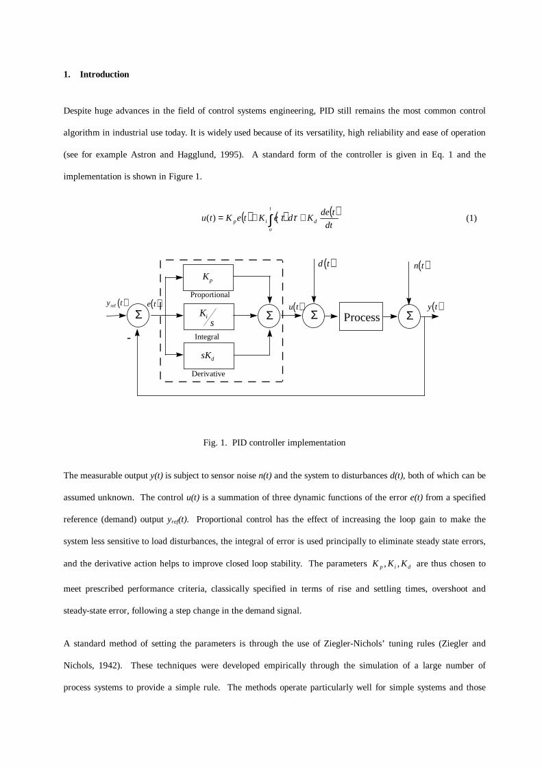
(see for example Astron and Hagglund, 1995). A standard form of the controller is given in Eq. 1 and the
implementation is shown in Figure 1.
( ) ( ) ( )∫ ++=t
o
dip dt
tdeKdeKteKtu ττ)( (1)
ProcessΣΣΣ Σ
-
Ks
i
Kp
sKd
( )d t ( )n t
( )y t( )u t( )e t( )y tref
Proportional
Integral
Derivative
Fig. 1. PID controller implementation
The measurable output y(t) is subject to sensor noise n(t) and the system to disturbances d(t), both of which can be
assumed unknown. The control u(t) is a summation of three dynamic functions of the error e(t) from a specified
reference (demand) output yref(t). Proportional control has the effect of increasing the loop gain to make the
system less sensitive to load disturbances, the integral of error is used principally to eliminate steady state errors,
and the derivative action helps to improve closed loop stability. The parameters dip KKK ,, are thus chosen to
meet prescribed performance criteria, classically specified in terms of rise and settling times, overshoot and
steady-state error, following a step change in the demand signal.
A standard method of setting the parameters is through the use of Ziegler-Nichols’ tuning rules (Ziegler and
Nichols, 1942). These techniques were developed empirically through the simulation of a large number of
process systems to provide a simple rule. The methods operate particularly well for simple systems and those
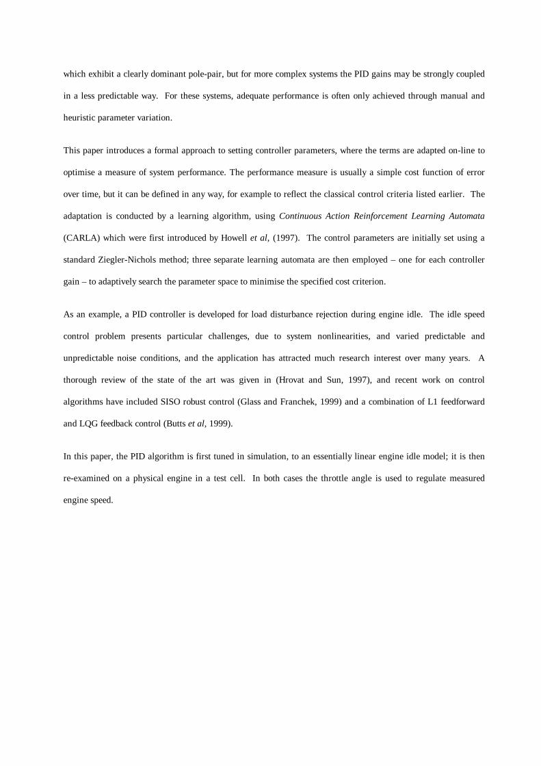
which exhibit a clearly dominant pole-pair, but for more complex systems the PID gains may be strongly coupled
in a less predictable way. For these systems, adequate performance is often only achieved through manual and
heuristic parameter variation.
This paper introduces a formal approach to setting controller parameters, where the terms are adapted on-line to
optimise a measure of system performance. The performance measure is usually a simple cost function of error
over time, but it can be defined in any way, for example to reflect the classical control criteria listed earlier. The
adaptation is conducted by a learning algorithm, using Continuous Action Reinforcement Learning Automata
(CARLA) which were first introduced by Howell et al, (1997). The control parameters are initially set using a
standard Ziegler-Nichols method; three separate learning automata are then employed – one for each controller
gain – to adaptively search the parameter space to minimise the specified cost criterion.
As an example, a PID controller is developed for load disturbance rejection during engine idle. The idle speed
control problem presents particular challenges, due to system nonlinearities, and varied predictable and
unpredictable noise conditions, and the application has attracted much research interest over many years. A
thorough review of the state of the art was given in (Hrovat and Sun, 1997), and recent work on control
algorithms have included SISO robust control (Glass and Franchek, 1999) and a combination of L1 feedforward
and LQG feedback control (Butts et al, 1999).
In this paper, the PID algorithm is first tuned in simulation, to an essentially linear engine idle model; it is then
re-examined on a physical engine in a test cell. In both cases the throttle angle is used to regulate measured
engine speed.

2. Continuous Action Reinforcement Learning Automata
The CARLA operates through interaction with a random or unknown environment by selecting actions in a
stochastic trial and error process. For applications that involve continuous parameters which can safely be varied
in an on-line environment, the CARLA technique can be considered to be more appropriate than alternatives. For
example, one such alternative, the genetic algorithm (Holland 1975) is a population based approach and thus
requires separate evaluation of each member in the population at each iteration. Also, although other methods
such as simulated annealing could be used, the CARLA has the advantage that it provides additional convergence
information through probabilitiy density functions.
CARLA was developed as an extension of the discrete stochastic learning automata methodology (see Narendra
and Thathachar, 1989 or Najim and Posnyak, 1994 for more details). CARLA replaces the discrete action space
with a continous one, making use of continuous probability distributions and hence making it more appropriate
for engineering applications that are inherently continuous in nature. The method has been successfully applied
to active suspension control (Howell et al, 1997) and digital filter design (Howell and Gordon, 1998). A typical
layout is shown in Figure 2.
ProcessRandom
Environment
Performance
Evaluation
CARLA 1
CARLA 2
CARLA n
M
( )f x1
( )f x2
( )f xn
M
RandomizedAction
Selector
Learning Sub-system
CostAction Set
x x xn1 2, , ,L
( ) ( ) ( ) f x f x f xn1 2, , ,LSet of Distributions
J
β
Fig. 2. Learning system

Each CARLA operates on a separate action – typically a parameter value in a model or controller – and the
automata set runs in a parallel implementation as shown, to determine multiple parameter values. The only
interconnection between CARLAs is through the environment and via a shared performance evaluation function.
Within each automata, each action has an associated probability density function f(x) that is used as the basis for
its selection. Action sets that produce an improvement in system performance invoke a high performance ‘score’
β, and thus through the learning sub-system have their probability of re-selection increased. This is achieved by
modifying f(x) through the use of a Gaussian neighbourhood function centred on the successful action. The
neighbourhood function increases the probability of the original action, and also the probability of actions ‘close’
to that selected; the assumption is that the performance surface over a range in each action is continuous and
slowly varying. As the system learns, the probability distribution generally converges to a single Gaussian
distribution around the desired parameter value.
Referring to the ith action (parameter), xi is defined on a pre-specified range xi(min), xi(max). For each
iteration k of the algorithm, the action xi(k) is chosen using the probability distribution function fi(xi,k), which is
initially uniform :
( ) [ ] otherwise
(max) (min), where
0
(min)(max)11, iiiii
ii
xxxxxxf
∈
−
= (2)
The action is selected by ( ) )(,)(
0
kzdxkxf i
kx
iii
i
=∫ (3)
where z varies uniformly in the range 0, 1.
With all n actions selected, the set is evaluated in the environment for a suitable time, and a scalar cost value J(k)
calculated according to some predefined cost function. Performance evaluation is then carried out using
( ) ( )
−−= 1 , ,0maxmin
minmed
med
JJ
kJJkβ (4)
where the cost )(kJ is compared with a memory set of R previous values from which minimum and median costs
Jmin , J med are extracted. The algorithm uses a reward / inaction rule, with action sets generating a cost below
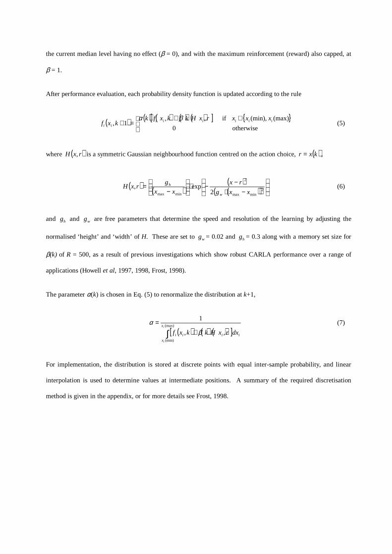
the current median level having no effect (β = 0), and with the maximum reinforcement (reward) also capped, at
β = 1.
After performance evaluation, each probability density function is updated according to the rule
( ) ( ) ( ) ( ) ( )[ ] otherwise
(max) (min), if
0
,,1, iiiiii
ii
xxxrxHkkxfkkxf
∈
+
=+βα
(5)
where ( )rxH , is a symmetric Gaussian neighbourhood function centred on the action choice, ( )kxr = ,
( ) ( )( )( )( )
−⋅−−⋅
−
=2
minmax
2
minmax 2exp,
xxg
rx
xx
grxH
w
h (6)
and gh and gw are free parameters that determine the speed and resolution of the learning by adjusting the
normalised ‘height’ and ‘width’ of H. These are set to gw = 0.02 and gh = 0.3 along with a memory set size for
β(k) of R = 500, as a result of previous investigations which show robust CARLA performance over a range of
applications (Howell et al, 1997, 1998, Frost, 1998).
The parameter α(k) is chosen in Eq. (5) to renormalize the distribution at k+1,
( ) ( ) ( )[ ]∫ +=
(max)
(min)
,,
1i
i
x
xiiii dxrxHkkxf β
α (7)
For implementation, the distribution is stored at discrete points with equal inter-sample probability, and linear
interpolation is used to determine values at intermediate positions. A summary of the required discretisation
method is given in the appendix, or for more details see Frost, 1998.

3. Engine Idle Speed Control
Vehicle spark ignition engines spend a large percentage of their time operating in the idle speed region. In this
condition the engine management system aims to maintain a constant idle speed in the presence of varying load
demands from electrical and mechanical devices, such as lights, air conditioning compressors, power steering
pumps and electric windows. Engines are inherently nonlinear, incorporating variable time delays and
discontinuities which make modelling difficult, and for this reason their control is well suited to optimisation
using learning algorithms.
3.1 Model Based Learning
For comparison with real engine data, and as a demonstration of CARLA operation, the technique is first tested
on a simple generic engine model. Cook and Powell (1988) presented a suitable structure, which relates change
in engine speed to changes in fuel spark and throttle, with the model linearised about a fixed idle speed. Figure 3
illustrates the model, with attached PID controller.
PID Controller Gi(s)
Inlet ManifoldDynamic
Ga(s)
Combustion Delay
+-
RotationalDynamics
Gr(s)
Pumping Feedback
++
Throttle
load D(t)(disturbance input)
Kn
++
∆F = 0Fuel
++
+
∆S = 0
Spark
0ref =∆V
Fig. 3. Engine idle speed simulation model

Component dynamics are taken as
( ) ( )Gi sK T
T s
p p
p
=+ 1
( )Gr ss
( ).
=+
20
35 1 ( )Ga s G ep
s= − τ (8)
where nominal system parameters are chosen: Tp = 0 05. , K Tp p = 9000 , Gp = 085. , Kn = × −1 10 4 with a
combustion time delay of 1.0=τ seconds. From earlier identification work, these settings are known to be
representative of the test engine which we will consider in Section 3.2, for an idle speed of 800rpm with no
electrical or mechanical load.
In this paper, control is applied via modulation of the throttle only, to minimise the change in engine speed (∆V)
in the presence of load torque variations D(t). Adopting the stability boundary method for Ziegler-Nichols tuning,
reference PID gains were obtained, and these are recorded in Table 1.
The CARLA algorithm is applied by defining three actions – one for each controller gain – with wide search
ranges, of ±200% of the Ziegler-Nichols settings. The optimisation was conducted by minimisation of integrated
time and squared error,
( )( ) τττ dVJT
2
0
∆⋅= ∫ (9)
over a suitably long period (T = 5 seconds) following an applied 10Nm step in load at t = 0. By time weighting
the error signal less emphasis is placed on the initial error, which is largely unavoidable, and greater emphasis on
reducing long duration oscillations.
Figure 4 shows how the probability density functions varied for each of the three parameters over a series of 3000
iterations. The proportional term has converged to a value close to the Ziegler-Nichols value, but the integral and
derivative terms have converged to one end of their range. Critically though, all three terms have converged
distinctly, and it can be shown that further learning only has the effect of reducing variance about the selected
values, to a minimum specified by H, ( )( )2minmax
2min xxgw −⋅=σ . Taking the three modal values of the final
distributions, the optimal controller is given along with a cost comparison in Table 1. Note the significant
performance benefit of the new controller – cost has been reduced by around 60%.

0
500
1000
1500
2000
2500
3000
−0.01
0
0.01
0.02
0.03
0
100
200
300
400
Iteration
Pro
b. D
ensi
ty
Proportional Gain
0
500
1000
1500
2000
2500
3000
−0.020
0.020.04
0.060.08
0.1
0
20
40
Iteration
Pro
b. D
ensi
ty
Integral Gain
0
500
1000
1500
2000
2500
3000
−50
510
1520
x 10−4
0
1000
2000
3000
Iteration
Pro
b. D
ensi
ty
Derivative Gain
Fig. 4. Controller parameter convergence

Table 1. Comparison of PID parameter settings and associated cost
Ziegler-Nichols CARLA Optimised
K p 0.0115 0.0137
Ki 0.04 0.1034
Kd 0.00082 0.0021
Cost, J 216 87
Figure 5 shows a comparison of responses to the load step; the benefits of increased integral and derivative action
are clear, with the error approaching zero more quickly and having lower initial overshoot in the learnt controller.
In this noise-free test however, high gains are suitable, so we might not expect the same trends in a physical
engine test.
Zeigler−Nichols Learnt Parameters
0 0.2 0.4 0.6 0.8 1 1.2 1.4 1.6 1.8 2−20
0
20
40
60
80
100
Spe
ed D
iffer
ence
from
Idle
(rp
m)
Time (s)
Fig. 5. Comparing controller performance for a 10Nm step change in load

3.2 On-Line Learning
To examine CARLA in the physical test environment, a Ford Zetec 1.8l engine was connected to a PC-based
digital control system in a test cell. Test equipment was arranged to emulate the measurement and control that
was simulated in section III(A); the equipment, operation and settings are illustrated in Figure 6 and summarised
below.
Air by-pass valve
Engine
DAC ADCPC / DSPControlSystem
to dummy loadAir by-pass input
Engine ManagementDevelopment Computer
( set fixed spark retard and fuelling )
ModifiedAlternator
Load resistor
Engine speed
Power Amp &PWM generator
EngineManagement
Module
Fig. 6. System implementation
(i) The control system consisted of a TMS320C40 digital signal processor, with Matlab, Simulink and dSPACE
software. A Simulink hardware-in-the-loop system was designed, measuring engine speed and supplying a
continuous control output to maintain idle at 800rpm. PID parameters were set on-line via a Matlab
program running the CARLA algorithm; to implement the controller, the derivative term was approximated
as ( )s
s1 200 1+.
(ii) A pulse-width modulated voltage was generated from the PC control signal, and applied to the engine air
bypass valve.

(iii) The engine management module was connected to a proprietary development computer, in order to over-ride
standard idle management. Spark retard was fixed at 13° before TDC, and fuelling set to vary with mass air
flow only, with no exhaust oxygen control. The air bypass valve lead was attached to a dummy load.
(iv) The alternator was attached to a low resistance (0.2Ω) load with its field voltage switched via a power
amplifier, by the PC / DSP control system.
For each learning iteration, new PID gains were set and allowed to settle before a 400 Watt load was switched on
for four seconds and then switched off. If during the test the control gains invoked an unstable engine response –
detected by ∆V > 200rpm – the system was stabilised by resetting the control parameters to Ziegler-Nichols
values, and the iteration was aborted. The cost was then evaluated according to time and speed error after both
transients, using a record of engine speed sampled at 1kHz :
( ) ( ) ( )∑∑==
∆⋅−+∆⋅=6000
4000
22000
0
2 4k
kkk
kk VtVtJ
After 1500 iterations – an on-line test of just over four hours – the cost had settled, and two of the three
probability distributions had converged. The cost – filtered using a 100 point moving mean – is shown in Figure
7, and the probability distributions are given in Figure 8.
0 500 1000 15000
1
2
3
4
5
6
7x 10
6
Iteration
Mea
n C
ost
Fig. 7. Mean cost reduction as a result of learning

0
500
1000
1500
2
3
4
5
6
x 10−3
0
500
1000
1500
Iteration
Pro
b. D
ensi
ty
Proportional Gain
0
500
1000
1500
00.5
11.5
22.5
3
x 10−3
0
500
1000
Iteration
Pro
b. D
ensi
ty
Integral Gain
0
500
1000
1500
0
1
2
3
4
5
x 10−4
0
5000
10000
15000
Iteration
Pro
b. D
ensi
ty
Derivative Gain
Fig. 8. Probability density function variation about Ziegler Nichols values
Ziegler-Nichols values :
Kp = 4×10⁻³
Ki = 1.5×10⁻³
Kd = 2.5 ×10⁻⁴

Again the P and D terms are distinct, with modal values Kp = 0.0028, Kd = 3.48×10⁻⁴. Interestingly, the integral
term is not well defined – the distribution indicates two candidate parameter ranges, with little cost difference
between them. Here we choose Ki = 0.0019, which is a modal peak from the wider of the two ranges. The choice
is nominal, but selecting from the wider range we might reasonably expect a more robust control solution. The
performance benefit of the learnt controller is shown separately for the load on and load off switches, in Figure 9.
Note the high amplitude disturbance process at the engine firing frequency of 27Hz. Compared with the engine
fundamental response frequency of around 1Hz, this is one complexity of the plant which may explain the lack of
convergence in Ki.
Ziegler−Nichols Learnt Parameters
0 0.2 0.4 0.6 0.8 1 1.2 1.4 1.6 1.8 2740
750
760
770
780
790
800
810
820
Time (s)
Eng
ine
Spe
ed (
rpm
)
Applying Load
Ziegler−Nichols Learnt Parameters
0 0.2 0.4 0.6 0.8 1 1.2 1.4 1.6 1.8 2780
790
800
810
820
830
840
850
Removing Load
Time (s)
Eng
ine
Spe
ed (
rpm
)
Fig. 9. Resulting improvement over Ziegler-Nichols
4. Concluding Remarks
Whilst it is recognised that the Ziegler-Nichols compensator is not optimised for the same criteria, the learnt
controller’s performance is excellent, with very different control gains achieving significant cost benefits. Also,
from this simple study and given the flexibility of CARLA, it seems likely that the system’s scope can be
extended. Restricting discussion to the engine idle application, feedforward control is a good candidate; some
engine loads can be anticipated (eg air conditioning pump demands), and CARLA might usefully be applied to
parametrise a model for feedforward control under expected load conditions.

The control algorithm itself can also be extended – for example by considering full state feedback; CARLA has
already been successfully employed in this way for optimising suspension control. More informally, gains could
be optimised for multiple feedback paths in a general classical controller; in addition to engine speed, manifold
pressure and mass air-flow may be measureable, and spark and fuelling actuation could be introduced. The
method would also have similar applications in the wider remit of engine management.
One notable disadvantage of learning is its specificity to the individual test environment; plant variations can
have significant implications for robustness. Again, potential solutions exist however – for example the learning
algorithm could be implemented on-line in service. By restricting gain ranges, it should be possible to slowly
adapt to individual plant variations throughout service life.
In summary, the continuous action reinforcement learning automata has been successfully applied to determine
PID parameters for engine idle speed control, both in simulation and in practice. The technique does not require
a-priori knowledge of the system dynamics, and it provides optimised control of complex nonlinear systems.
5. References
Astron, K.J. and T. Hagglund (1995). PID Controllers: Theory, Design, and Tuning, ISA, Research Triangle
Park, NC, USA.
Butts, K.R., N. Sivashankar and J. Sun (1999). Application of l1 optimal control to the engine idle speed control
problem, IEEE Transactions on Control Systems Technology, Vol. 7, No. 2, pp 258-270.
Cook, J.A. and B.K. Powell (1988). Modelling of an internal combustion engine for control analysis, IEEE
Control Systems Magazine, Vol. 8, No. 4, pp. 20-26.
Frost, G.P. (1998). Stochastic Optimization of Vehicle Suspension Control Systems via Learning Automata, PhD
Dissertation. Aeronautical and Automotive Engineering Department. Loughborough University.
Glass, J.W. and M.A. Franchek (1999). NARMAX modelling and robust control of internal combustion engines,
International Journal of Control, Vol. 72, No. 4, pp 289-304.
Holland, J.H. (1975). Adaptation in Natural and Artificial Systems, The University of Michigan Press, Ann
Arbor.

Howell, M.N., G.P. Frost, T.J. Gordon and Q.H. Wu (1997). Continuous action reinforcement learning applied to
vehicle suspension control, Mechatronics, Vol. 7, No. 3, pp 263-276.
Howell, M.N. and T.J. Gordon (1998). Continuous learning automata and adaptive digital filter design,
Proceedings of Control ’98, Swansea, UK.
Hrovat, D. and J. Sun (1997). Models and control methodologies for IC engine idle speed control design, Control
Engineering Practice, Vol. 5, No. 8, pp 1093-1100.
Najim, K. and A.S. Posnyak (1994). Learning Automata; Theory and Applications, Pergamon, Oxford.
Narendra, K. and M.A.L. Thathachar (1989). Learning Automata: An Introduction, Prentice-Hall, London.
Ziegler, J.G. and N.B. Nichols (1942). Optimum setting for Automatic Controllers, Trans. ASME, Vol. 64, pp.
759-768.

Appendix
In order to implement CARLA, the probability distributions fi must be stored and updated at discrete sample
points. The most efficient data storage can be achieved using equal inter-sample probability rather than equal
sampling on xi, but this is at some computational expense, as the sampled vector xi must be redefined after each
iteration k, acording to the updated distribution fi(xi,k+1).
The data management is carried out by first executing the algorithm as described in Section 2, but using α = 1
and evaluating equations (5) - (7) at the N current sampled points xi(k). A new set of sample points xi(k+1) is
then selected sequentially from xi(min) to xi(max); with regard to Figure A1 (and dispensing with the subscript i),
x1 = x(min), xN = x(max) and intermediate samples are defined for j = 1, N-1 by the following :
f(x, k+1)
x
x1(k)= x1(k+1)
= x(min)
x3(k)x2(k+1) xj(k+1)
xj+1(k+1)
Fig. A1. Re-sampling on the linearly interpolated probability density function
jN
Aa j
j −−
=+
11 (A1)
( ) ( )[ ] ( )( ) ( )( )[ ] 111 1,1,115.0 +++ =+−++−+ jjjjj akxfkxfkxkx (A2)
11 ++ += jjj aAA (A3)
Here aj refers to the jth intersample probability, and Aj records the cumulative re-sampled probability at j (A1=0).
In each case, equation (A2) is solved for xj+1(k+1) by interpolating ( )( )1,1 ++ kxf j between known values on

f(xj,k+1), and solving the resulting quadratic equation. The sequential re-calculation of target intersample
probability – equation (A1) – prevents cumulative interpolation errors from corrupting the probability distribution
function as it develops with iterations. This algorithm was used successfully in the paper using the relatively
small sample set N = 100.


![[PID] PID Control - Good Tuning - A Pocket Guide](https://img.pdfslide.net/doc/110x75/577d2a661a28ab4e1ea914b1/pid-pid-control-good-tuning-a-pocket-guide.jpg)


![C6-PID Controller Tuning[1]](https://img.pdfslide.net/doc/110x75/55cf9497550346f57ba30ba9/c6-pid-controller-tuning1.jpg)