Embed Size (px)
Citation preview

TI 2007-054/1 Tinbergen Institute Discussion Paper
On Mergers in Consumer Search Markets
Maarten C.W. Janssen1
José Luis Moraga-González2*
1 Erasmus University Rotterdam, and Tinbergen Institute; 2 University of Groningen, and CESifo. * Associate research fellow TI.

Tinbergen Institute The Tinbergen Institute is the institute for economic research of the Erasmus Universiteit Rotterdam, Universiteit van Amsterdam, and Vrije Universiteit Amsterdam. Tinbergen Institute Amsterdam Roetersstraat 31 1018 WB Amsterdam The Netherlands Tel.: +31(0)20 551 3500 Fax: +31(0)20 551 3555 Tinbergen Institute Rotterdam Burg. Oudlaan 50 3062 PA Rotterdam The Netherlands Tel.: +31(0)10 408 8900 Fax: +31(0)10 408 9031 Most TI discussion papers can be downloaded at http://www.tinbergen.nl.

On Mergers in Consumer Search Markets∗
Maarten C. W. Janssen†
Erasmus University Rotterdam and Tinbergen Institute
Jose Luis Moraga-Gonzalez‡
University of Groningen and CESifo
June 2007
Abstract
We study mergers in a market where N firms sell a homogeneous good and consumerssearch sequentially to discover prices. The main motivation for such an analysis is that mergersgenerally affect market prices and thereby, in a search environment, the search behavior ofconsumers. Endogenous changes in consumer search may strengthen, or alternatively, offsetthe primary effects of a merger. Our main result is that the level of search costs are crucialin determining the incentives of firms to merge and the welfare implications of mergers. Whensearch costs are relatively small, mergers turn out not to be profitable for the merging firms. Ifsearch costs are relatively high instead, a merger causes a fall in average price and this triggerssearch. As a result, non-shoppers who didn’t find it worthwhile to search in the pre-mergersituation, start searching post-merger. We show that this change in the search composition ofdemand makes mergers incentive-compatible for the firms and, in some cases, socially desirable.
Keywords: consumer search, mergers, price dispersionJEL Classification: D40, D83, L13
∗We thank Chaim Fershtman, Mike Waterson, Matthijs Wildenbeest, Chris Wilson and Hugo Boff for their valuablecomments on the subject. The paper has also benefited from presentations at Pompeu Fabra University, PortugueseCompetition Authority and the 2007 International Industrial Organization Conference (Savannah).
†Erasmus University Rotterdam and Tinbergen Institute. P.O.Box 1738, 3000 DR Rotterdam, The Netherlands.E-mail: [email protected]
‡Department of Economics, University of Groningen, P.O. Box 9700 AV Groningen, The Netherlands. E-mail:[email protected]
1
1 Introduction
The literature on the incentives of firms to merge and on the economic effects of mergers is quite
extensive. One basic point that is coming back throughout this literature is that mergers strengthen
firms’ market power so that, in the absence of any offsetting effect, mergers are detrimental from a
welfare point of view. Another basic point relates to the firms’ incentives to merge.1 Salant, Switzer
and Reynolds (1983) studied such incentives using a Cournot model with homogeneous product
sellers. They derived the paradoxical result that quantity-setting firms do not have an incentive to
merge, except in the case where the merger leads to a monopoly. The paradox arises because in
the post-merger equilibrium the non-merging firms increase their output relative to the pre-merger
situation, which tends to put sufficient pressure on prices so as to make merging unprofitable.
This result, known as the merger paradox, had an immediate response in the work of Deneckere
and Davidson (1985) and Perry and Porter (1985). Deneckere and Davidson studied mergers in a
horizontally differentiated products market with price-setting firms. They showed that the strategic
nature of the decision variables has an important bearing on the results. Indeed, price-setting firms
may have an incentive to merge because price increases of the merging firms are accompanied by
price increases of the non-merging firms. The price increases, of course, also imply that total welfare
is always lower in the post-merger market. Perry and Porter (1985), building on Williamson (1968),
explicitly modelled the cost efficiencies which arise from economies of sharing assets in a setting
with homogeneous product markets. They found conditions under which an incentive to merge
exists and mergers are socially desirable. In antitrust economics, this reduction-in-costs argument
in favor of mergers has been called the efficiency defense.2
So far the study of mergers has exclusively focused on markets with perfect price information.
Casual empiricism suggests the contrary, i.e. that consumers typically lack price information and
have to incur significant search costs to get it. By incorporating consumer search activity into a
model of mergers, this paper provides new and interesting perspectives on the study of the economic
effects of mergers. First, ceteris paribus, mergers have an effect on (the distribution of) prices; as
price setting and search intensity are endogenously determined in consumer search markets, we
show that changes in search behavior due to price variations can reinforce or offset the initial effect
on prices. Second, one of the consequences of consumers having to search to discover prices is the
1For a survey of the literature on the unilateral effects of mergers see Ivaldi, Jullien, Rey, Seabright and Tirole(2003a).
2See also the papers of Farrell and Shapiro (1990) and McAfee and Williams (1992).
2
failure of the “law of one price” (see e.g. Burdett and Judd, 1983; Stahl, 1989; Reinganum, 1979).3
When the market outcome is characterized by a distribution of prices, consumers who search more
intensively end up paying lower prices on average than consumers who search little. We show that
the impact of mergers on consumer welfare may differ across consumer types, i.e., mergers may
have distributional effects at the demand side. To the best of our knowledge, this is the first paper
addressing these two issues.
To contrast our context with the two reactions to the merger paradox outlined above, we assume
that mergers do not yield any cost efficiencies and that the firms market homogeneous products. We
study mergers in the classical sequential consumer search model of Stahl (1989) with N retailers,
but we relax the assumption that the first price quotation is costless (see Janssen et al., 2005). On
the demand side of the market there are two types of consumers, namely, consumers who search
at no cost and thus are fully informed at all times, and consumers who must pay a positive search
cost each time they search. In this model, there is a unique mixed strategy equilibrium but, in
contrast to the original paper by Stahl (1989), this equilibrium may come in three types. The
distinct types of equilibrium differ in the level of prices that can be sustained in the market as well
as in the search composition of demand. In fact, the departure from Stahl’s original setup has the
implication that consumers with high search cost do not necessarily participate in the market.
We show that the economic effects of mergers in consumer search markets hinge upon the level
of search costs. When search costs are relatively low, in equilibrium all consumers participate in
the market. In this case, mergers do not affect demand, but just consumer prices and firms’ profits.
It turns out that mergers are unprofitable in this instance of low search costs and therefore we
may expect that mergers do not to take place in these types of market. This result thus confirms
that the merger paradox continues to hold in markets where search costs are relatively small and
unimportant.
When search costs are instead relatively high, some consumers find it prohibitive to participate
in the market and do not search or buy in equilibrium. In this case, a merger results in a change in
the search composition of demand such that merging firms may obtain larger profits in the post-
merger situation than in the pre-merger one. This is because a merger results in a lowering of the
average price in the market, which is precisely the price that triggers search. Non-shoppers who
3The existence of price dispersion for seemingly identical goods has been extensively documented in empiricalwork (see e.g., Stigler (1961) and Pratt et al. (1979) for early studies and Sorensen (2000) and Lach (2001) for morerecent work).
3
didn’t find it worthwhile to search in the pre-merger situation, start searching post-merger. Relative
to the pre-merger situation, the ratio of active high search cost (non-price-sensitive) consumers to
low search cost (price-sensitive) consumers increases in the post-merger market and this explains the
increase-in-profits result. The paper thus shows that the merger paradox does not hold when search
costs are relatively important, even if products are homogeneous and there is no cost efficiency to
be gained from the merger.
Incentive-compatible mergers turn out to lead to an increase in consumer participation and this
has the potential to make them even socially desirable (from a total surplus point of view). We
show that this is always the case when demand is inelastic, while with downward sloping demand
only if the share of fully informed consumers is low. Moreover, as the different groups of consumers
exert externalities on one another, mergers have interesting distributional effects. Indeed, we find
that mergers hurt low search cost consumers because they end up paying higher prices on average,
but at the same time they benefit high search cost consumers because they pay lower prices on
average. The paper shows that these results are robust to several changes in the basic model.
The main thesis of this paper is that mergers may have novel and interesting effects when search
costs are relatively large. How large search costs are in real-world markets is therefore a natural
empirical question. Several authors (Hong and Shum, 2006; Hortacsu and Syverson, 2004; and
Moraga-Gonzalez and Wildenbeest, 2007) have recently proposed structural methods to estimate
search costs. Although this literature is still in its infancy, the results show that consumers do not
to search much, which suggests that search costs may be larger than expected. For example, in
a study of some on-line markets for memory chips, Moraga-Gonzalez and Wildenbeest (2007) find
that only around 10% of the consumers seems to search intensively. This finding is in line with the
results reported by Johnson et al. (2004), who studied consumer click-through behavior online. In
a study of the market for prescription drugs, Sorensen (2001) reports a similar finding that only
between 5% to 10% of the consumers conduct an exhaustive search. On the basis of this evidence,
our results for the case that search costs are relatively high may be important for the way mergers
are analyzed by anti-trust authorities.4
4The fact that search costs may be so high that consumers stop searching may explain some of the recent develop-ments in the market for telephone directory assistance services in quite a number of European countries. Traditionally,the incumbent operators provided these services and consumers could access it by dialing 118. New firms wanted toenter this industry, but claimed they would be unsuccessful as long as the incumbent firm could continue to use the118 number as all consumers knew this number by heart and automatically dialed it in case they needed this sortof service. Regulators, insisting on the need for more competition in the market, forbid incumbent firms to continueusing the 118 number. The typical consumer now has to search for a number to call to as well as for the price ofthe service. It is already a few years since the 118 number was removed, and the size of the market has shrunk
4

The remainder of the paper is organized as follows. Section 2 describes the consumer search
model we use and Section 3 discusses the special case of unit demand. Section 4 then briefly discusses
the equilibrium analysis of the general model with downward sloping demand, while Section 5 delves
into the two questions related to the incentives to merge and the welfare implications of mergers.
Section 6 develops an extension of the basic model where we replace the set of identical high search
cost consumers with a heterogeneous group of consumers who differ in their search cost. We show
that the results discussed above remain the same and that the only change is with respect to
the search behavior of the consumers. Section 7 concludes and provides a discussion of the main
assumptions of the paper. Proofs are relegated to the appendix.
2 The Model
We study mergers in the standard consumer search model of Stahl (1989), but we assume that
all price quotations are costly to obtain (as in Janssen et al., 2005).5 The features of the model
are as follows. There are N ≥ 3 firms that produce a homogeneous good at constant returns to
scale. Their identical unit cost can be normalized to zero and prices can be interpreted as price-
to-cost margins. There is a unit mass of buyers and we assume that buyers’ demand curves are
given by D(p), with D′(p) < 0, where p is the price at which the consumer decides to buy. In
some of the analysis we assume for convenience that demand is linear, i.e., D(p) = a − bp, with
a > 0, b > 0. It will be useful to denote the revenue function as R(p) = pD(p); we assume that R(p)
is monotonically increasing up to the monopoly price, denoted, pm. Let R−1(·) be the inverse of the
revenue function. The surplus of a consumer who buys at price p is denoted as CS(p) =∫∞p D(p)dp.
A proportion λ ∈ (0, 1) of the consumers has zero opportunity cost of time and therefore searches
for prices costlessly. These consumers are referred to as ‘shoppers’ or low search cost consumers.
The rest of the buyers, referred to as ‘non-shoppers’ or high search cost consumers, must pay search
cost c > 0 to observe every price quotation they get, including the first one. Non-shoppers search
for lower prices sequentially, i.e., a buyer first decides whether to sample a first firm or not and
then, upon observation of the price of the first firm, decides whether to search for a second price
considerably relative to the old days.5The assumption that consumers obtain the first price quotation at no cost has been widely adopted in the search
literature and it boils down to assuming all consumers participate in the market so industry demand is inelastic. Asshown in Janssen et al. (2005) this assumption is not without loss of generality. In fact, when search is truly costlynot all consumers may search because their search cost may be too high compared to the value of the product andthe price they expect to pay for the good. In those cases, the market will no longer be covered and industry demandwill typically be elastic, which is a more natural outcome.
5

or not, and so on. To avoid trivialities, we assume that if all firms priced at marginal cost then all
consumers would search once and buy at the encountered firm, i.e., CS(0) =∫∞0 D(p)dp > c,
Firms and buyers play the following game. An individual firm chooses its price taking price
choices of the rivals as well as consumers’ search behavior as given. An individual buyer forms
conjectures about the distribution of prices in the market and decides on his/her optimal search
strategy. We confine ourselves to the analysis of symmetric Nash equilibria. The distribution of
prices charged by a firm is denoted by F (p), its density by f(p) and the lower and the upper bound
of its support by p and p, respectively. It is obvious that firms will never set prices above the
monopoly price.
Before moving to the study of the effects of mergers, we need to address the issue of whether
merging firms wish to continue to operate two retail stores or else prefer to shut down one of the
stores. The difference is that in the first case the merged entity would be in control of two prices,
while in the second case the merged firm would control only one price. To answer this question, we
need to make assumptions about the information consumers have in connection with the merger.
In what follows, we shall assume that, if a merger occurs, consumers know (i) that two firms have
merged, and (ii) the identity of the merging firms. Of course, since we are modelling mergers in a
search environment, we shall assume consumers don’t know the prices of the merging firms without
searching. Assumption (i) captures the idea that consumers’ conjectures about the gains from
search must be correct in equilibrium. Assumption (ii) implies that consumers can choose whether
to search for prices among the merged entities or else search for prices among the non-merging
firms. The next proposition argues that the merging firms do not have an incentive to continue to
operate two independent stores.
Proposition 1 Suppose two firms merge and that consumers know the identity of the merging
firms; then, the merged entity prefers to be in control of a single price rather than in control of two
prices. As a result, it is optimal for the merging firms to close down one of their stores.
The idea behind the proof of this result, which is placed in the Appendix, is as follows. Since
merging does not bring any cost reduction, in the post-merger market consumers must be indifferent
between shopping at the merging stores and shopping at the non-merging stores for otherwise the
pricing of either type of firm would not be optimal. It turns out that if the merging firms control
two prices in the post-merger equilibrium, the unilateral incentives of the merging stores lead them
to charge higher prices on average than the non-merging firms, which constitutes a contradiction as
6

consumers wouldn’t then wish to visit any of the merging firms. Hence, appealing to this result, in
the rest of the paper we analyze the case where the merged firms shut down one of their stores.6,7
We note that Proposition 1 extends to situations where consumers know a merger has taken
place in the market but do not know the identity of the merging firms. We spell out the basic ideas
behind this statement in the Conclusions section.
3 Mergers: the simple case of unit-demand
We start our discussion on the incentives of firms to merge and on the collective effects of mergers by
looking at the simple case of unit demand (D(p) = 1, for all p ≤ v and 0 otherwise). When demand
is inelastic, there aren’t dead-weight-losses and therefore the analysis of mergers is relatively simple;
the paper will deal with elastic demands in Sections 4 and 5 and the role of this section is to put
forward the main issues in the possibly most simple setting.
Janssen et al. (2005) present a complete characterization of equilibria in the unit-demand case.
Their findings, described in a compact way, are as follows. There is a unique symmetric equilibrium.
When search costs are relatively low, non-shoppers participate in the market with probability one.
We refer to this situation as an equilibrium with full consumer participation. In that case firms
obtain an expected profit Eπ = (1−λ)ρN/N and the reservation price ρN (indexed by N to indicate
its dependency on N) can be calculated explicitly as:
ρN =c
1−∫ 1
0
dy1+bNyN−1
< v, (1)
where b = λ/(1 − λ). The ratio of shoppers to non-shoppers will be important for our analysis
since it tells us something about the composition of demand. When c is large enough so that (1)
is not satisfied, a partial consumer participation equilibrium exists. In this type of equilibrium,
an individual firm obtains a profit Eπ = µN (1 − λ)v/N, where µN is the probability with which
6In the proof of this result we assume that the merged entity cannot commit to charge the same price in thetwo stores. Under this assumption, the merged entity is tempted to increase the price at one of the stores and thistemptation can only be eliminated by shutting down one of the shops. However, the result in Proposition 1 canbe extended to the case in which the merged firm can commit to charging the same price in the two stores. Theargument is similar because, in that case, the merged entity would have a larger share of non-shoppers and wouldthus charge higher prices (cf. Baye et al., 1992 ).
7Proposition 1 should also hold if firms marketed differentiated products (cf. Anderson and Renault, 1999). Theidea is that a firm that operates two stores internalizes the externalities between shops and so is tempted to chargehigher prices than the rival firms. As a result, a consumer who knows the incentives of the firms would rather searchamong the non-merging firms.
7

non-shoppers search and is implicitly determined by the solution to
1−∫ 1
0
dy
1 + 1µbNyN−1
=c
v, (2)
which states that the incremental gain from searching one time rather than not searching at all
equals the marginal cost of search. Notice that the LHS of (2) is a continuously decreasing function
of µ, going from 1 to some positive number (for details see Janssen et al., 2005).
The unit-demand case is convenient because there are no welfare effects associated to price
changes other than those related to the rate of participation of the non-shoppers. As a result,
total surplus generated in the market takes a simple expression: TS = λv + µN (1− λ)(v− c). This
expression reflects two facts. One, a shopper always acquires one unit from the cheaper supplier
thus generating a surplus equal to v (this surplus is somehow divided between the supplier and
consumer); two, a non-shopper only buys with probability µN ≤ 1, in which case a surplus of v−c is
generated. Janssen et al. (2005) show that (as a comparative statics exercise) µN is non-increasing
in N. Therefore, in a full consumer participation equilibrium total surplus is independent of N , but
in a partial consumer participation equilibrium total surplus if higher when N is smaller.
To our knowledge, the incentives of firms to merge have so far not been studied in a search
model. In this context of unit demand, we can show that in a full participation equilibrium firms
do not have an incentive to merge, whereas they do have an incentive to merge in a subset of
the parameter space where the equilibrium involves only partial consumer participation. Taking
this observation along with the remarks on welfare above, this means that whenever firms have an
incentive to merge, total welfare increases. Moreover, if merging does not increase total surplus,
firms do not have an incentive to merge. Thus, from the point of view of social welfare, the
incentives to merge are insufficient in this case of unit-demand: there are situations where mergers
would be socially desirable from a total surplus point of view, but they do not occur as the firms
involved do not have an incentive to merge.
We start by showing that in a full participation equilibrium firms do not have an incentive
to merge. Before the merger, an individual firm’s profit is given by (1 − λ)ρN+1/(N + 1), while
post-merger profits of a typical firm are (1 − λ)ρN/N. As a result, firms do not have an incentive
to merge when the collective post-merger profits of the merging firms is lower than the joint pre-
merger profits, i.e., when 2ρN+1/(N + 1) > ρN/N. Using the reservation price formula in (1), this
8

condition requires thatc/(N + 1)
1−∫ 1
0
dy1+b(N+1)yN
>c/2N
1−∫ 1
0
dy1+bNyN−1
.
This can be rewritten as
N − 1− 2N
∫ 1
0
dy
1 + bNyN−1+ (N + 1)
∫ 1
0
dy
1 + b(N + 1)yN> 0.
Or, rearranging, as
(N − 1)(
1−∫ 1
0
dy
1 + bNyN−1
)> (N + 1)
(∫ 1
0
dy
1 + bNyN−1−∫ 1
0
dy
1 + b(N + 1)yN
).
It is easy to see that the LHS of this inequality is positive. Thus, if the RHS is negative, the claim
that mergers are not incentive-compatible when search costs are low follows. To show the RHS is
indeed negative, rewrite it as∫ 1
0
[byN−1((N + 1)y −N)
(1 + b(N + 1)yN ) (1 + bNyN−1)
]dy. (3)
Note that 1+ b(N +1)yN and 1+ bNyN−1 are both positive and strictly increasing in y. Therefore,
we can follow the proof of Proposition 1 of Janssen and Moraga-Gonzalez (2004) to show that the
expression in (3) is indeed negative. In particular,∫ 1
0
[byN−1((N + 1)y −N)
(1 + b(N + 1)yN ) (1 + bNyN−1)
]dy
=∫ N
N+1
0
[byN−1((N + 1)y −N)
(1 + b(N + 1)yN ) (1 + bNyN−1)
]dy −
∫ 1
NN+1
[byN−1(N − (N + 1)y)
(1 + b(N + 1)yN ) (1 + bNyN−1)
]dy
≤∫ N
N+1
0
byN−1((N + 1)y −N)(1 + b NN
(N+1)N−1
)2 dy −∫ 1
NN+1
byN−1(N − (N + 1)y)(1 + b NN
(N+1)N−1
)2 dy
=b(
1 + b NN
(N+1)N−1
)2
∫ 1
0yN−1((N + 1)y −N)dy = 0.
Therefore, firms do not have an incentive to merge when the search cost is sufficiently low. In
addition, there are no welfare gains to be derived from mergers.
We next show that firms may have an incentive to merge in a partial participation equilibrium,
i.e., when the search cost is sufficiently large. In this case, in the pre-merger situation an individual
firm obtains a profit of µN+1(1−λ)v/(N+1), while post-merger profits are µN (1−λ)v/N. Therefore,
mergers are beneficial for the merging firms if µN/N > 2µN+1/(N + 1). From (2), we know that
9

µN is the solution to ∫ 1
0
dy
1 + bµNyN−1
= 1− c
v
and that µN+1 solves ∫ 1
0
dy
1 + bµ(N + 1)yN
= 1− c
v
As proven above, ∫ 1
0
dy
1 + bµNyN−1
>
∫ 1
0
dy
1 + bµ(N + 1)yN
for all µ
Given these equilibrium restrictions on how the participation rate of the non-shoppers is determined,
we conclude that merging is profitable for the firms if∫ 1
0
dy
1 + bµN
NyN−1<
∫ 1
0
dy
1 + 2 bµN
NyN.
This condition holds if
bN
µN
∫yN−1(1− 2y)dy(
1 + bµN
NyN−1)(
1 + 2bµN
NyN) > 0.
Or
bNµN
∫yN−1(1− 2y)dy
(µN + bNyN−1) (µN + 2bNyN )> 0. (4)
We now show that this inequality holds when µN is sufficiently small. From the remarks above
after equation (2), it follows that for given values of b and N, µN can always be chosen close enough
to 0 by taking c close enough to v. At µN = 0, the expression (4) equals 0; let us now show that
(4) increases in µN in a neighborhood of µN = 0. Taking the derivative of (4) with respect to µN
yields ∫ 1
0
bNyN−1(1− 2y)[2b2N2y2N−1 − µ2
N
](µN + bNyN−1)2 (µN + 2bNyN )2
dy
For µN close to 0, the sign of this expression will be determined by the sign of∫ 1
0
yN−1(1− 2y)4b4N4y4N−2
[2b2N2y2N−1
]dy
=∫ 1
0
1− 2y
2b2N2yNdy =
∫ 1/2
0
1− 2y
2b2N2yNdy −
∫ 1
1/2
2y − 12b2N2yN
dy
>1
2b2N2(
12
)N(∫ 1/2
0(1− 2y) dy −
∫ 1
1/2(2y − 1) dy
)
=2N−1
b2N2
∫ 1
0(1− 2y) dy = 0.
10

This proves that for c values close enough to v, µN/N > 2µN+1/(N + 1) and therefore mergers are
incentive-compatible for the merging firms.
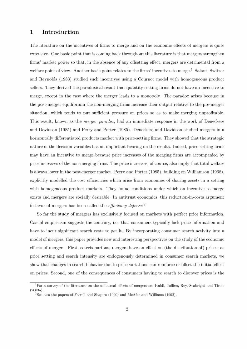
At this point we would like to note that the range of values of c for which the firms would
rather merge is of course larger. To illustrate this point, we have computed numerically the region
of parameters for which mergers would be incentive-compatible. The results appear in Figure 1.
Figure 1: Parameters for which mergers are profitable and welfare improving (λ = 0.5).
We finish this section by elaborating on the redistributive effects of a profitable merger. When
mergers are incentive-compatible, non-shoppers are indifferent between searching and not searching
so we can deduct industry profits µN (1−λ)v from total surplus to obtain the surplus of the shoppers:
λv − µN (1 − λ)c. Since µN+1 < µN , it follows that shoppers are worse off after a merger. It is
important to note that this reduction in the welfare of shoppers is not due to a genuine increase
in prices because expected price remains constant. The decrease is due to the fact that the firms’
incentives to compete for the informed consumers weaken as fewer firms remain in the market and
therefore, the chance of observing relatively low prices decreases as well. This harms fully informed
consumers as they buy at the lowest observed price in the market.
4 Equilibria
We now analyze our general model with downward sloping demand. In this Section we characterize
the symmetric equilibrium and present a theoretical innovation: compared to Stahl (1989), we find
that there are three types of symmetric equilibrium. The distinct types of equilibrium differ in
the price levels that can be sustained and hold for different magnitudes of search costs. Later in
11

Section 5 we study mergers.
We start by characterizing optimal consumer search. For this purpose, we invoke some results
already known in the consumer search literature.
Lemma 1 If there exists a symmetric equilibrium, then (i) non-shoppers search either once surely
or mix between searching and not searching, and (ii) firms set prices randomly drawn from an
atomless price distribution.
Proof. For a proof of these results see Stahl (1989) and Janssen et al. (2005). �
The ideas underlying this lemma are as follows. If non-shoppers were not active at all, firms
would have no other equilibrium choice than charging the competitive price. In that case, non-
shoppers’ behavior would not be optimal. Now consider that in equilibrium a non-shopper walks
away from a firm j which is charging a price pj . This implies that the expected gains from searching
further at price pj are higher than the search cost, i.e.,∫ pj
p (CS(p) − CS(pj))dF (p) > c. Since all
non-shoppers are identical, no consumer would remain at firm j so charging pj cannot be optimal.
Notice that these two remarks together imply that non-shoppers either search for one price with
probability one or mix between searching once and not searching at all. In either case, they do not
compare prices. Consider now the strategy of a firm and suppose that all firms charge the same
price p > 0. Since shoppers compare all prices in the market, it is readily seen that an individual
firm would gain by charging a price slightly less than p; all firms charging p = 0 cannot be an
equilibrium either since a deviant firm would gain by slightly increasing its price (the firm would
sell to those non-shoppers who happen to venture its store and make a strictly positive profit).
In conclusion, symmetric equilibrium implies that firms mix in prices and non-shoppers either
search for one price surely or mix between searching and not searching. In what follows we examine
the characterization and the existence of equilibrium.
Case a: High search cost
Suppose that non-shoppers mix between searching and not searching. Let µ ∈ (0, 1) denote the
probability with which non-shoppers are active in the market. In this case the expected payoff to
a firm i from charging price pi when its rivals choose a random pricing strategy according to the
cumulative distribution F (·) is
πi(pi, F (pi)) = R(pi)[µ(1− λ)
N+ λ(1− F (pi))N−1
]. (5)
12

The expression in square-brackets represents the quantity firm i expects to sell at price pi. The
firm expects to serve the shoppers when it happens to be the case that its price is lower than its
rivals’ prices; likewise, the firm expects to sell to the non-shoppers when they happen to visit its
store.
In equilibrium, a firm must be indifferent between charging any price in the support of F (·);
this indifference condition allows us to calculate the equilibrium price distribution:
F (p) = 1−(
µ(1− λ)λN
R(p)−R(p)R(p)
) 1N−1
. (6)
Given that consumers are indifferent between searching and not searching, the upper bound of the
price distribution must be equal to the monopoly price pm for otherwise a firm charging a price
equal to an upper bound p < pm would gain by increasing its price. The lower bound of the price
distribution can easily be calculated by setting F (p) = 0 and solving for p.
The cumulative distribution (6) represents optimal firm pricing, given consumer search behavior.
We now turn to find the conditions under which the assumed buyer search activity is optimal. For
non-shoppers to mix between searching and not searching, it must be the case that the surplus
they expect to get in the market is equal to the search cost, i.e.,∫ pm
pCS(p)f(p)dp = c. (7)
We can use the variable change z = 1− F (p) to rewrite condition (7) as follows:∫ 1
0CS
(R−1
(R(pm)
1 + λNµ(1−λ)z
N−1
))dz = c. (8)
Let us denote the LHS of (8) as βN (µ), which denotes the incremental gains to a non-shopper from
entering the market. Note that this function also depends on λ and demand parameters; to save
on space we will not write this dependency unless necessary. Since CS(·) is a decreasing function
while R−1(·) is an increasing function, it is straightforward to verify that βN (µ) decreases in µ. It
is also easy to check that βN (µ) converges to CS(0) as µ → 0; likewise, as µ approaches 1, βN (µ)
converges to a strictly positive number denoted βN (1). This leads to the following existence and
uniqueness result.
Proposition 2 Let CS(0) > c > βN (1). Then there exists a unique symmetric mixed strategy
equilibrium where firms prices are distributed according to the cdf given in (6) and non-shoppers
mix between searching for one price with probability µ and not searching at all with the remaining
13

probability, with µ given by the solution to (8). In equilibrium an individual firm obtains an expected
profit equal to π = µ(1 − λ)R(pm)/N, non-shoppers obtain an expected surplus equal to zero and
shoppers obtain and expected surplus equal to∫ pm
p CS(p)N(1− F (p))N−1f(p)dp > 0.
Case b: Low search cost
Suppose that non-shoppers search for one price with probability 1, as in Stahl (1989). In this case
the expected payoff to a firm i from charging price pi when its rivals choose a random pricing
strategy according to the cumulative distribution F (·) is
πi(pi, F (pi)) = R(pi)[1− λ
N+ λ(1− F (pi))N−1
]. (9)
The interpretation of this expression is similar to that in (5).
Proceeding as before we can calculate the equilibrium price distribution:
F (p) = 1−(
1− λ
λN
R(p)−R(p)R(p)
) 1N−1
. (10)
The cdf in (10) represents optimal firm pricing given that non-shoppers search once surely. Let
us now check when such behavior is optimal for consumers. If consumers do not search further
it is because the expected gains from search are lower than the search cost. Let us define the
reservation price ρ as the price that makes a non-shopper indifferent between searching once more
and accepting ρ right away; this price satisfies:∫ ρ
p[CS(p)− CS(ρ)] f(p)dp = c. (11)
Notice that the LHS of (11) is increasing in ρ so that ρ is increasing in c. If in equilibrium consumers
do not search further it is indeed because firms do charge prices not greater than ρ because otherwise
consumers would go on with their search. As a result, p ≤ ρ; we also know that prices above the
monopoly price are not optimal either. These two observations imply that the maximum price
charged in the market must satisfy
p ≤ min{ρ, pm}. (12)
Consider the search cost c such that the reservation price which solves (11) equals the monopoly
price. This search cost satisfies
c =∫ pm
p[CS(p)− CS(pm)] f(p)dp (13)
14

Or
c =∫ pm
pCS(p)f(p)dp− CS(pm) = βN (1)− CS(pm) (14)
For search costs c ≥ c, the upper bound of the equilibrium price distribution p is equal to pm.
For non-shoppers to search for one price surely it must be the case that, ex-ante, they expect to
get sufficient surplus to cover the search cost, i.e.,∫ pm
pCS(p)f(p)dp > c. (15)
which imposes the condition that βN (1) > c.
When c < c, the upper bound of the equilibrium price distribution p is equal to ρ, where ρ
solves (11), which can be rewritten as∫ ρ
pCS(p)f(p)dp = c + CS(ρ) (16)
For non-shoppers to search for one price surely it must be the case that, ex-ante, they expect to
get sufficient surplus to cover the search cost, i.e.,∫ ρ
pCS(p)f(p)dp > c. (17)
which holds when (16) is satisfied. Then we have the following result:
Proposition 3 (a) Let 0 < c < βN (1) − CS(pm). Then there exists a unique symmetric mixed
strategy equilibrium where firms prices are distributed according to the cdf given in (10) with p = ρ
and non-shoppers search for one price with probability 1. The reservation value ρ solves (11).
(b) Let βN (1) − CS(pm) < c < βN (1). Then there exists a unique symmetric mixed strategy
equilibrium where firms prices are distributed according to the cdf given in (10) with p = pm and
non-shoppers search for one price with probability 1.
In equilibrium firms obtain expected profits equal to π = µ(1 − λ)R(p)/N, non-shoppers obtain
an expected surplus equal to∫ pp CS(p)f(p)dp > 0 and shoppers obtain an expected surplus equal to∫ p
p CS(p)N(1− F (p))N−1f(p)dp > 0.
Our results show there is a unique symmetric equilibrium where consumers may either search
once surely, or mix between searching and not searching. This depends on the market parameters,
in particular when search cost is low, consumers search once surely and their threat to search
further restricts pricing in that the maximum price charged in the market is the reservation price
15

ρ < pm. When search cost is moderate, consumers search also one time surely but the firms can
safely charge prices up to the monopoly price, since buyers’ threat to continue searching is not very
effective. When search costs are sufficiently high, non-shoppers expect prices to be that high that
they are indifferent between searching and not searching.
5 Mergers
The analysis of mergers in the unit-demand case is, of course, highly simplified, as it does not
incorporate the consumer surplus effects of the price changes driven by mergers. In what follows,
we show that the results of Section 3 generally hold true so that the absence of these consumer
surplus effects is not essential for the argument to hold. The general idea is that in consumer
search markets mergers give firms incentives to lower average prices so that consumers who were
not searching in the pre-merger situation may find it worthwhile to initiate search. This boost-
in-demand effect of mergers may make them profitable for the merging firms as well as socially
desirable.
Proposition 4 Assume that D(p) = a − bp. (i) For any a, b, λ and N , if 0 < c < βN (1), then
πN+1 > πN/2 so merging is not individually rational. (ii) For any a, b, λ and N there exists
c ∈ (βN (1), CS(0)) such that πN+1 < πN/2 for all c ≥ c, i.e., merging is individually rational for
a pair of firms.
The proof of this result is in the Appendix. We first prove that mergers are not incentive
compatible when the search cost is low. The reason is that in this case of low search costs a merger
results in a lowering of the reservation value so the profits of the merging firms fall after the merger.
Secondly, we prove that when search costs are relatively high, a merger changes the composition
of demand in such a way that the non-shoppers to shoppers ratio increases, which implies that
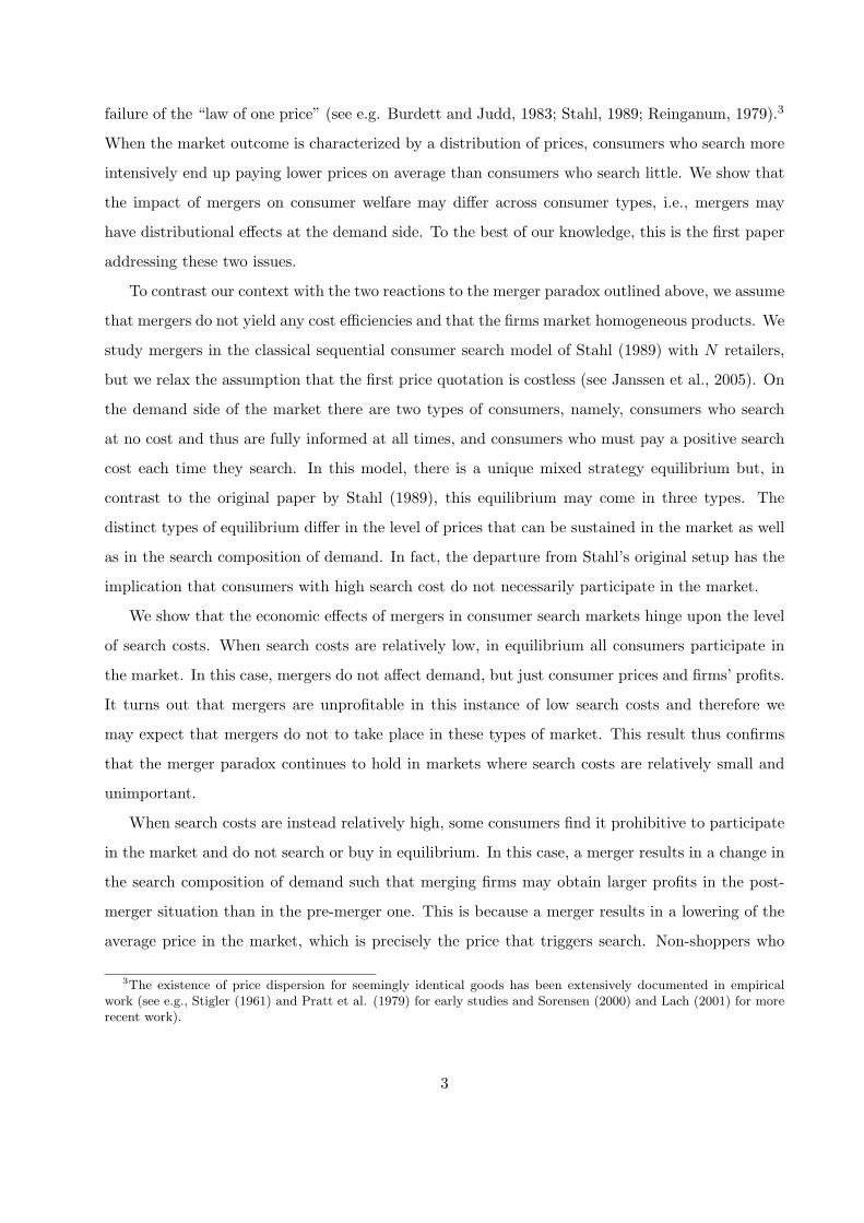
firms can raise their prices and thereby their profits. The idea behind the proof is in Figure 2.
The decreasing solid curves denote the non-shoppers’ incremental gains from searching once rather
than not searching at all; these gains are given in equation (8). The thicker curve shows these
gains in the pre-merger situation while the thinner curve shows them in the post-merger situation.
To understand why this schedule is decreasing notice that when µ → 0, only shoppers are left
in the market so pricing must be competitive; in that case, the incremental gains from searching
over not searching are highest and equal CS(0). As the number of non-shoppers increases, pricing
becomes more monopolistic and the gains from participation decrease. The search intensities of
16

the non-shoppers in the pre- and post-merger markets are then given by the intersection of these
curves with the cost of search; these search intensities are µN and µN+1, respectively.
A merger is incentive-compatible when each of the merging firms obtains a post-merger profit
that is larger than the pre-merger profits, i.e., when R(pm)(1−λ)µN+1/N+1 > R(pm)(1−λ)µN/2N .
This implies that for a profitable merger it must be the case that µN+1 < µN (N + 1)/2N , or in
other words, it must be that a sufficiently large new group of non-shoppers will find it worthwhile
to start searching post-merger so that the market expands. In the proof we show that when c is
sufficiently large this is indeed the case.
Figure 2: Profitable mergers and high search costs.
Our second result discusses who benefits and who looses because of the mergers.
Proposition 5 Assume that D(p) = a − bp and that c ∈ (βN (1), CS(0)). Then a merger leads to
an increase in industry profits and to a decrease in the surplus of the shoppers; the surplus of the
non-shoppers remains constant.
Proposition 5 shows that the social welfare implications of mergers are complex: the collective
profit of the firms increases at the expense of the surplus of the shoppers while non-shoppers
continue to obtain zero surplus. In the unit demand case it was easy to show that the increase in
industry profits offsets the decrease in the surplus of the shoppers. Unfortunately, that proof does
not extend easily to the new situation with elastic demand. Our next result shows that when the
17

market hosts few shoppers, welfare increases as a result of the merger; simulation results (some of
which are presented after the proposition) suggest that this welfare result is much more general.
Proposition 6 Assume that D(p) = a− bp, and that c ∈ (βN (1), CS(0)). Then limλ→0(TS(N)−
TS(N + 1)) > 0.
Numerical analysis of the model reveals that the result in Proposition 6 holds also in markets
with an fraction number of shoppers. To illustrate this, Table 1 shows the relevant equilibrium
variables when 50% of the consumers are shoppers and 50% are non-shoppers. For this example we
take demand to be q = 1 − 0.9p and the search cost c = 0.4. For these parameters, non-shoppers
enter the market with probability µ. The Table shows that mergers increase the participation rate
of the non-shoppers. This leads to a rise in firm profits and aggregate welfare. Again, shoppers
lose when mergers occur.
N=2 N=3 N=4 N=5 N=6µ 0.7912 0.4776 0.2631 0.1354 0.0659Eπ 0.0549 0.0221 0.0091 0.0037 0.0015CSshoppers 0.4372 0.4821 0.5142 0.5339 0.5449Welfare 0.3285 0.3074 0.2936 0.2857 0.2816Notes:
Parameters are a = 1, b = 0.9, c = 0.4 and λ = 0.5.Welfare is TS = λECSshoppers + NEπ.
Table 1: Equilibrium values (model with linear demand)
6 Search cost heterogeneity
So far we have assumed that all non-shoppers have identical search cost. In reality, search costs
will be more smoothly distributed across the consumer population. In this section, we relax the
equal-search-cost assumption and consider the case where non-shoppers have different search costs.
To keep things relatively simple, we introduce search cost heterogeneity in a way that extends the
analysis in the main body of the paper. In the concluding section we will discuss more informally
some results that can be obtained in a more general search model.
We consider a situation where consumers demand one unit of the good at most, and their
common valuation is equal to v. Let search costs be uniformly distributed in the interval [c, c], with
v ≥ c > c > 0, and assume that in equilibrium there exists a consumer with search cost c who is
18
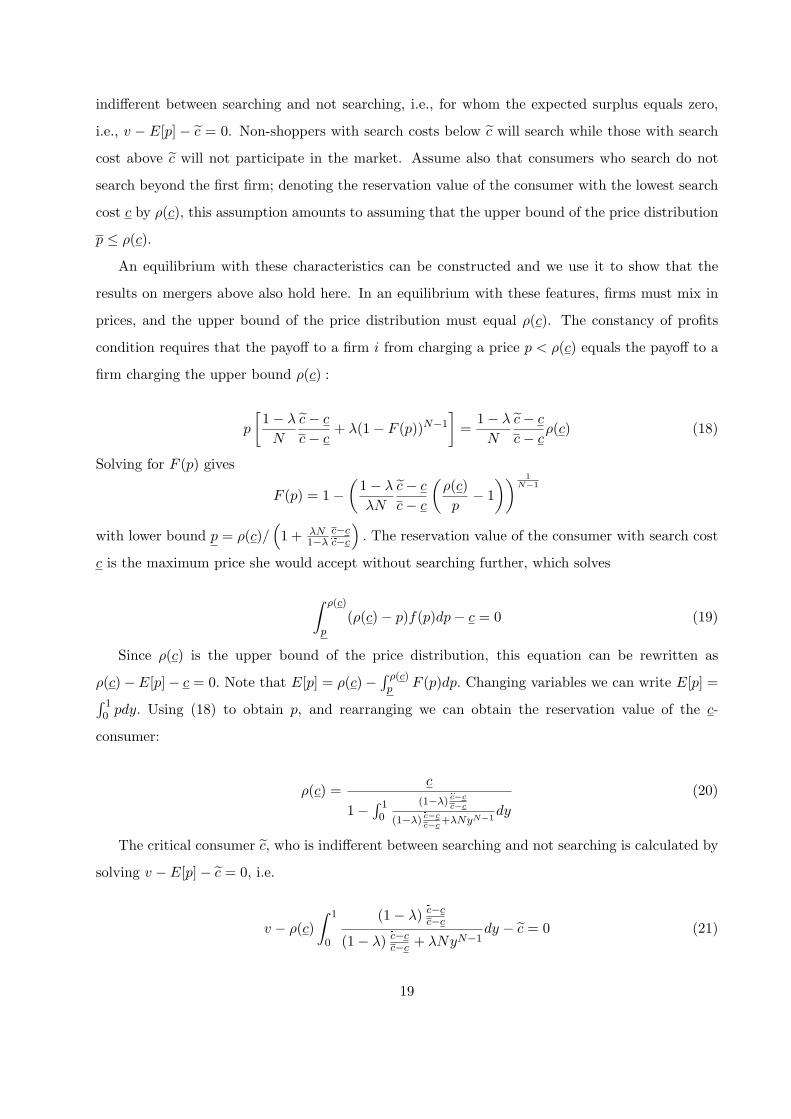
indifferent between searching and not searching, i.e., for whom the expected surplus equals zero,
i.e., v − E[p] − c = 0. Non-shoppers with search costs below c will search while those with search
cost above c will not participate in the market. Assume also that consumers who search do not
search beyond the first firm; denoting the reservation value of the consumer with the lowest search
cost c by ρ(c), this assumption amounts to assuming that the upper bound of the price distribution
p ≤ ρ(c).
An equilibrium with these characteristics can be constructed and we use it to show that the
results on mergers above also hold here. In an equilibrium with these features, firms must mix in
prices, and the upper bound of the price distribution must equal ρ(c). The constancy of profits
condition requires that the payoff to a firm i from charging a price p < ρ(c) equals the payoff to a
firm charging the upper bound ρ(c) :
p
[1− λ
N
c− c
c− c+ λ(1− F (p))N−1
]=
1− λ
N
c− c
c− cρ(c) (18)
Solving for F (p) gives
F (p) = 1−(
1− λ
λN
c− c
c− c
(ρ(c)p
− 1)) 1
N−1
with lower bound p = ρ(c)/(1 + λN
1−λc−cec−c
). The reservation value of the consumer with search cost
c is the maximum price she would accept without searching further, which solves
∫ ρ(c)
p(ρ(c)− p)f(p)dp− c = 0 (19)
Since ρ(c) is the upper bound of the price distribution, this equation can be rewritten as
ρ(c)−E[p]− c = 0. Note that E[p] = ρ(c)−∫ ρ(c)p F (p)dp. Changing variables we can write E[p] =∫ 1
0 pdy. Using (18) to obtain p, and rearranging we can obtain the reservation value of the c-
consumer:
ρ(c) =c
1−∫ 10
(1−λ) ec−cc−c
(1−λ) ec−cc−c
+λNyN−1dy
(20)
The critical consumer c, who is indifferent between searching and not searching is calculated by
solving v − E[p]− c = 0, i.e.
v − ρ(c)∫ 1
0
(1− λ) ec−cc−c
(1− λ) ec−cc−c + λNyN−1
dy − c = 0 (21)
19

Equations (18) to (21) define a candidate equilibrium. To complete the characterization we need
to show that no firm has an incentive to charge prices outside the support of the price distribution.
It is obvious that a firm would not gain by charging a price less than the lower bound p. Consider
a firm deviating by charging a price p above the upper bound, i.e., p > ρ(c). To calculate the
payoff of the deviant, notice that, given the strategy of the other firms, the deviant firm will not
attract any of the shoppers; moreover, note that some of the non-shoppers, in particular those with
reservation prices less than p, will continue to search. Let c be the search cost of the consumer
whose reservation value is p, i.e., p satisfies p − E[p] − c = 0. If p is so large that c > c then
no buyer will buy from the deviant. If p is not so high, then the payoff to the deviant would be
Eπd(p > ρ(c)) = p1−λN
ec−bcc−c . At p = ρ(c), this profit expression equals the equilibrium profits. Taking
the derivative of this profit formula with respect to p yields 1−λN
ec−2bp+E[p]c−c = 1−λ
Nec−2bc−E[p]
c−c , which is
clearly negative for search cost distributions with a small range.
We are now ready to study the effects of mergers on firm profits and welfare. The profits of a
firm in this market are given by Eπ = 1−λN
ecN−cc−c ρ(c), where, as usual, we index c by the subscript
N to indicate the dependency of c on N. Comparing profits in the pre-merger and post-merger
situations reveals that merging is individually rational for a pair of firms if ec(N+1)−cN+1 < ec(N)−c
2N .
Welfare in this market is given by the expression W = λv +∫ecN
cv−cc−cdc.
N=2 N=3 N=4 N=5 N=6 N=7c 6.45082 6.14807 5.91674 5.75535 5.6496 5.58415ρ(c) 9.04918 9.35193 9.58326 9.74465 9.8504 9.91585E[p] 3.54918 3.85193 4.08326 4.24465 4.3504 4.41585Eπ 1.07552 0.505056 0.24961 0.12442 0.0614 0.0298016W 5.95667 5.67658 5.44713 5.27912 5.1655 5.09379Notes:Parameters are v = 10, c = 5.5, c = 7.5;λ = 0.5.
Table 2: Equilibrium values (model with search cost heterogeneity)
Table 2 shows how mergers can be incentive-compatible and welfare improving also with search
cost heterogeneity. The table shows how the endogenous variables vary when we increase the
number of firms. It can be seen that the number of non-shoppers participating in the market
declines as N increases. This causes the maximum price to increase as well as the mean price.
Firm profits decrease and welfare increase as the number of firms in the market rises. In this case,
mergers are incentive-compatible and socially desirable.
20

7 Discussion and Conclusion
We have studied mergers in a market where N firms sell a homogeneous good and consumers search
sequentially to discover prices. The main motivation for this study has been that mergers generally
affect market prices and thereby, in a search environment, the search intensity of the consumers.
We have seen that endogenous changes in consumer search behavior have the potential to reinforce
or, alternatively, offset the initial price effects of a merger. Interestingly, when search costs are
relatively large, a merger results in a decrease in the expected price and since this is precisely the
price which triggers search for consumers with relatively high search cost, non-shoppers who didn’t
find it worthwhile to search in the pre-merger situation, start searching post-merger. We have seen
how this “boost-in-demand” effect of mergers can make mergers incentive-compatible for the firms
and socially desirable. This result seems to be relatively robust, since it holds under unit demand,
elastic demand, and search cost heterogeneity.
To the best of our knowledge this is the first paper on mergers in markets with search frictions.
Along the way, we have made a number of simplifying assumptions. For example, we have assumed
that consumers know the identity of the merging firms. Building on the distinction between the
gains from searching among the merged firms and the gains form searching among the non-merging
firms, we have proven that the merging firms do not have an incentive to continue to operate two
stores. The problem is that a firm which operates two shops is tempted to increase one of its prices
all the way up to the monopoly price which, as a result, would drive consumers away from the
merging firms. We have argued that this problem would persist even if the merging firms could
credibly commit not to charge different prices at the two different shops, since still in this case the
merging firms would be charging on average higher prices than the non-merging firms.
An interesting question is what would happen if consumers could not tell which firms have
merged. It turns out that the merging firms are strictly better off by letting consumers know about
the merger for otherwise non-shoppers’ incentives to enter the market after the merger would be
weakened and the potential for profitable mergers would be reduced. The idea is that consumers,
knowing that a merger has occurred, would expect one of the (merging) stores to be charging the
monopoly price, which increases market average prices and lowers incentives to participate in the
market altogether.
[IRELAND PAPER] [MERGER WAVES]
Another simplifying assumption relates to the fact that consumers are quite homogeneous.
21

Although we have analyzed some form of search cost heterogeneity, we have not addressed the
more general situation where valuations and search costs of consumers follow some (arbitrary)
distribution. Such a more general analysis is interesting as it will bring out other ways in which
the composition of demand may change because of a merger. From the analysis in this paper we
know that the ratio of consumers who search only once relative to the consumers who compare
more prices is an important factor determining market outcomes. In the present paper, this ratio
can change after a merger, as some consumers will start searching after the merger instead of not
searching at all. In a more general setup, it may very well be the case that a larger share of
consumers becomes more prone not to search thoroughly (i.e. accept higher prices right away)
after a merger.8 We hope to pursue this line of inquiry in future work.
8 Appendix
Proof of Proposition 1. We first show that firms will quote prices in such a way that non-
shoppers will not search beyond the first firm. Let F 1i (p) and F 2
i (p) be the (mixed) strategies
of the two shops of the merged entity; likewise, let F−i(p) denote other firms’ (mixed) strategies.
Let the supports of these mixed strategies be given by [p1i, p1
i ], [p2i, p2
i ] and [p−i, p−i], respectively.9
Consider a consumer who has observed a price p. The consumer’s gains from searching one more
time depend on whether the consumer ventures one of the stores of the merged entity, or else one of
the shops of the non-merging firms. Let f1i (x) and f2
i (x) denote the price densities corresponding
to the merged entity’s shops. A consumer who ventures one of the merged entity’s shops should
then expect a price according to the density function[f1
i (x) + f2i (x)
]/2. Therefore, the gains from
search for a consumer who searches randomly among the merging firms are
Φi(p) =∫ p
0[CS(x)− CS(p)]
[f1
i (x) + f2i (x)
]/2dx;
likewise, the gains from search for a consumer who searches one of the merging firms after having
visited the other merged firm are
Φji (p) =
∫ p
0[CS(x)− CS(p)] f j
i (x)dx, j = 1, 2; (22)
8Of course whether a consumer searches further or not will in general depend on which price realization he/sheobserves.
9Standard arguments can be used to show that the supports of these pricing strategies must be compact and thatthere should not have mass points, except the strategies of the merging firms possibly having a mass point at theupper bound of their support.
22

finally, the gains from searching among the non-merging firms are
Φ−i(p) =∫ p
0[CS(x)− CS(p)] f−i(x)dx
where f−i(x) denotes the price density function of a non-merging firm.
Given these expressions, we can define the reservation price of the non-shoppers for continued
search among the different search alternatives: the price ρi (respectively ρji , ρ−i, j = 1, 2) which
solves Φi(ρ) = c (respectively Φji (ρ) = c, Φ−i(ρ) = c, j = 1, 2). Similar arguments as in Stahl
(1989) imply that none of the firms will charge a price above min{ρ1i , ρ
2i , ρ−i, p
m} so non-shoppers
will visit one of the stores and stop searching there. The main point to realize here is that a firm
charging max{p1i , p
2i , p−i} will not sell to any consumers if this price is above min{ρ1
i , ρ2i , ρ−i} as
non-shoppers will continue searching.
There are then three cases to be distinguished: (i) non-shoppers prefer to visit first one of
the shops of the merged entity, (ii) non-shoppers prefer to first visit one of the non-merged firms
and (iii) non-shoppers are indifferent between shops, whether from a merged firm or not. We now
discuss these cases in turn.
(i) Suppose non-shoppers prefer to visit first one of the shops of the merged firm. In this case,
the non-merging stores will only sell to the shoppers, if at all, in which case the price distribution of
a non-merging store should be degenerated at the marginal cost. This constitutes a contradiction,
however, as then the non-shoppers would prefer to visit one of the non-merging stores as well.
(ii) Consider next the case that non-shoppers prefer to visit first one of the non-merged firms.
This implies that the merged firm will only attract the shoppers who are informed about all the
prices. In this case –if it can happen at all in equilibrium– the merged firm (weakly) prefers not to
set different prices in the two stores as the store with the highest price does not generate any sales.
(iii) So, if in equilibrium the merged firm prefers to set different prices in the two stores, it must
be the case that the non-shoppers are indifferent between visiting one of the non-merged firms and
visiting one of the merged firm’s stores. In this case, the payoff to the merging firm setting prices
p1i , p
2i (supposing p1
i ≤ p2i without loss of generality) would be
π(p1i , p
2i ;F−i(·)) =
{p1
i
[1−λN + λ(1− F−i(p1
i ))N−2
]+ p2
i1−λN if p1
i < p2i
p1i
[1−λN + λ
2 (1− F−i(p1i ))
N−2]+ p2
i
[1−λN + λ
2 (1− F−i(p2i ))
N−2]
if p1i = p2
i
(23)
This profit expression is easily understood on the basis of the following two observations. First,
23

note that each retail store of the merged entity attracts a share 1/N of the non-shoppers, who
come in proportion 1− λ. Second, suppose that p1i < p2
i . The cheapest store, in this case store 1,
happens to attract all the shoppers when the price at this store is the lowest in the market, i.e.,
with probability (1 − F−i(p1i ))
N−2. When p1i = p2
i , the shoppers are indifferent between the two
stores so on average half of them show up at store 1 and the other half at store 2.
It is straightforward to see that the profit expression in (23) is monotonically increasing in p2i
hence the distribution of prices at one of the stores must be degenerated at the upper bound of the
price distribution. Given this, it is readily seen that, when choosing p1i , the merged entity faces
exactly the same tradeoff as the rival firms so in equilibrium we must have F 1i (p) = F−i(p) for all
p. From standard arguments it follows that the price distribution F−i(p) must be atomless, with
convex support and mean price E[p] ≤ p.
Consider now a consumer contemplating to venture one of the merging stores. Since buyer
conjectures must be correct in equilibrium, this consumer should expect to observe a price equal to
(p + E[p])/2 at one of the merging stores. Hence, the expected price at one of the merging stores
will be higher than the expected market price so non-shoppers should rather visit one of the rival
firms. It then follows that merging firms have an incentive to commit to setting one price and one
way to make this commitment credible is to shut down one of the stores.10 �
Proof of Proposition 4. Part (i). We first prove that mergers are not incentive compatible when
search costs are relatively low, in particular when c < βN (1). Note that in this case non-shoppers
participate with probability 1 and the equilibrium characterizations is given in Proposition 3.
The equilibrium price cdf is
FN (p) = 1−(
(1− λ)λN
R(p)−R(p)R(p)
) 1N−1
where p denotes the upper bound of the price distribution. When search costs are relatively low,
it follows from Proposition 3 that p is either equal to the monopoly price pm or to the reservation
price ρN < pm. where ρN is given by the solution to (11). For mergers to be incentive-compatible
we need that p(1− λ)/2N be greater than p(1− λ)/(N + 1). When p = pm it follows immediately
that mergers are not profitable. Consider now the case in which p = ρN . Equation (11) can be
10As argued in the main text, we are assuming here that the merging firms cannot commit to charge the sameprice in the two stores (cf. footnote 6).
24

rewritten as
a2
2b− a
2
(∫ ρN
ppfN (p)dp
)− 1
2
(∫ ρN
pp(a− bp)fN (p)dp
)− (a− bρN )2
2b= c (24)
Let
I1 =∫ ρN
ppfN (p)dp
I2 =∫ ρN
pp(a− bp)fN (p)dp
Using the change of variables z = 1− F (p), these two integrals can be written as follows:
I1 =a
2b− 1
2b
∫ 1
0
√a2 − 4bρN (a− bρN )
1 + λN1−λzN−1
dz
I2 =∫ 1
0
ρN (a− bρN )1 + λN
1−λzN−1dz
Plugging these in (5) we get
a2
2b− a
2
(a
2b− 1
2b
∫ 1
0
√a2 − 4bρN (a− bρN )
1 + λN1−λzN−1
dz
)− 1
2
(∫ 1
0
ρN (a− bρN )1 + λN
1−λzN−1dz
)− (a− bρN )2
2b= c
Or
a2
4b+
a
4b
∫ 1
0
√a2 − 4bρN (a− bρN )
1 + λN1−λzN−1
dz − 12
(∫ 1
0
ρN (a− bρN )1 + λN
1−λzN−1dz
)− (a− bρN )2
2b= c (25)
Let us denote the LHS of (25) by H(·). We are interested in the derivative of ρN with respect
to N. Actually we want to prove that ρN increases in N. Using the implicit function theorem we
havedρN
dN= −
∂H(·)∂N
∂H(·)∂ρN
Above in the paper we have proven that∫ 10
11+ λN
1−λzN−1
dz increases in N. Likewise,∫ 10
√a2 − 4bρ(a−bρ)
1+ λN1−λ
zN−1
decreases in N. As a result, H(·) decreases in N.
25

It thus remains to prove that ∂H(·)∂ρN
> 0.
∂H(·)∂ρ
=a
4b
∫ 1
0
1
2√
a2 − 4bρN (a−bρN )
1+ λN1−λ
zN−1
−4b(a− 2bρN )1 + λN
1−λzN−1dz − 1
2
∫ 1
0
(a− 2bρN )1 + λN
1−λzN−1dz +
a
2+
a− 2bρN
2
(26)
=a− 2bρN
2
(1−
∫ 1
0
11 + λN
1−λzN−1dz
)+
a
2
1−∫ 1
0
1√a2 − 4bρN (a−bρN )
1+ λN1−λ
zN−1
(a− 2bρN )1 + λN
1−λzN−1dz
(27)
Let us look at the integrals in (8). We know that 1−∫ 10
11+ λN
1−λzN−1
dz > 0. For the second integral
we have
1−∫ 1
0
1√a2 − 4bρN (a−bρN )
1+ λN1−λ
zN−1
(a− 2bρN )1 + λN
1−λzN−1dz > 1− (a− 2bρN )√
a2 − 4bρN (a− bρN )= 0
This proves that ∂H(·)∂ρN
> 0. The desired result follows.
Part (ii). We now prove that when search costs lie in the range c ∈ (βN (1) , CS(0)) mergers
may be profitable for the merging firms. First note that in equilibrium non-shoppers randomize
between searching and not searching in both the pre-merger and the post-merger equilibria. The
participation rate of the non-shoppers in the pre-merger and post-merger situations, µN+1 and µN ,
are given by the solution to the following equations:∫ pm
pN+1
CS(p)fN+1(p)dp = c (28)
∫ pm
pN
CS(p)fN (p)dp = c, (29)
respectively. Therefore, it must be the case that (using the variable change z = 1− F (p))
∫ 1
0CS
R−1
R(pm)
1 + λ(N+1)µN+1(1−λ)z
N
=∫ 1
0CS
(R−1
(R(pm)
1 + λNµN (1−λ)z
N−1
))(30)
26
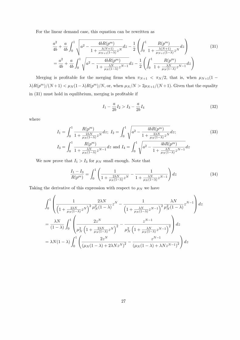
For the linear demand case, this equation can be rewritten as
a2
4b+
a
4b
∫ 1
0
√√√√a2 − 4bR(pm)
1 + λ(N+1)µN+1(1−λ)z
Ndz − 1
2
∫ 1
0
R(pm)
1 + λ(N+1)µN+1(1−λ)z
Ndz
(31)
=a2
4b+
a
4b
∫ 1
0
√a2 − 4bR(pm)
1 + λNµN (1−λ)z
N−1dz − 1
2
(∫ 1
0
R(pm)1 + λN
µN (1−λ)zN−1
dz
)
Merging is profitable for the merging firms when πN+1 < πN/2, that is, when µN+1(1 −
λ)R(pm)/(N +1) < µN (1−λ)R(pm)/N, or, when µN/N > 2µN+1/(N +1). Given that the equality
in (31) must hold in equilibrium, merging is profitable if
I1 −a
2bI2 > I3 −
a
2bI4 (32)
where
I1 =∫ 1
0
R(pm)1 + 2λN
µN (1−λ)zN
dz; I2 =∫ 1
0
√a2 − 4bR(pm)
1 + 2λNµN (1−λ)z
Ndz; (33)
I3 =∫ 1
0
R(pm)1 + λN
µN (1−λ)zN−1
dz and I4 =∫ 1
0
√a2 − 4bR(pm)
1 + λNµN (1−λ)z
N−1dz
We now prove that I1 > I3 for µN small enough. Note that
I1 − I3
R(pm)=∫ 1
0
(1
1 + 2λNµN (1−λ)z
N− 1
1 + λNµN (1−λ)z
N−1
)dz (34)
Taking the derivative of this expression with respect to µN we have
∫ 1
0
1(1 + 2λN
µN (1−λ)zN)2
2λN
µ2N (1− λ)
zN − 1(1 + λN
µN (1−λ)zN−1
)2
λN
µ2N (1− λ)
zN−1
dz
=λN
(1− λ)
∫ 1
0
2zN
µ2N
(1 + 2λN
µN (1−λ)zN)2 −
zN−1
µ2N
(1 + λN
µN (1−λ)zN−1
)2
dz
= λN(1− λ)∫ 1
0
(2zN
(µN (1− λ) + 2λNzN )2− zN−1
(µN (1− λ) + λNzN−1)2
)dz
27

In a neighborhood of µN = 0, the sign of this expression equals the sign of∫ 1
0
(2zN
(2λNzN )2− zN−1
(λNzN−1)2
)dz =
1λ2N2
∫ 1
0
(1
2zN− 1
zN−1
)dz =
1λ2N2
∫ 1
0
zN−1(1− 2z)2z2N−1
dz =1
λ2N2
(∫ 1
0
1− 2z
2zNdz
)=
1λ2N2
(∫ 1/2
0
1− 2z
2zNdz −
∫ 1
1/2
2z − 12zN
dz
)>
2N−1
λ2N2
(∫ 1/2
0(1− 2z) dz −
∫ 1
1/2(2z − 1)dz
)=
2N−1
λ2N2
(∫ 1
0(1− 2z) dz
)= 0.
To complete the argument, we now prove that I2 < I4 for µN sufficiently small. That is, we
need to show that∫ 1
0
√a2 − 4bR(pm)
1 + λNµN (1−λ)z
N−1dz −
∫ 1
0
√a2 − 4bR(pm)
1 + 2λNµN (1−λ)z
Ndz > 0
Taking the derivative of this expression with respect to µN we have∫ 1
0
1
2√
a2 − 4bR(pm)
1+ λNµN (1−λ)
zN−1
4bR(pm)(1 + λN
µN (1−λ)zN−1
)2
−λN
µ2N (1− λ)
zN−1dz
−∫ 1
0
1
2√
a2 − 4bR(pm)
1+ 2λNµN (1−λ)
zN
4bR(pm)(1 + 2λN
µN (1−λ)zN)2
−2λN
µ2N (1− λ)
zNdz
The sign of this expression is equal to the sign of∫ 1
0
1
2√
a2 − 4bR(pm)
1+ 2λNµN (1−λ)
zN
1(µN + 2λN
(1−λ)zN)2 2zNdz−
∫ 1
0
1
2√
a2 − 4bR(pm)
1+ λNµN (1−λ)
zN−1
1(µN + λN
(1−λ)zN−1
)2 zN−1dz
In a neighborhood of µN = 0, this reduces to∫ 1
0
12a
1(2λN(1−λ)z
N)2 2zNdz −
∫ 1
0
12a
1(λN
(1−λ)zN−1
)2 zN−1dz
=(1− λ)2
2aλ2N2
(∫ 1
0
(1
2zN− 1
zN−1
)dz
)=
(1− λ)2
2aλ2N2
(∫ 1
0
zN−1(1− 2z)2z2N−1
dz
)> 0
where the last inequality follows from the proof above that I1 > I3. Since µN → 0 as c → CS(0),
the result follows. �
Proof of Proposition 5. Industry profits are equal to µN (1 − λ)R(pm) and they are clearly
increasing in µN . As µN > µN+1, if c > βN (1), the result on profits follows trivially. The result for
28

the shoppers simply follows from the fact that if c > βN (1), they are indifferent between searching
and not searching so that their expected surplus equals 0.
Consider now the expected surplus of the shoppers, which is equal to∫ pm
p(N)
(a− bp)2
2bdFN (p) (35)
where FN (p) denotes the distribution of the minimum price of a random draw of size N when N
firms operate in the market.
As before, denoting R(p) = p(a− bp), we rewrite (35) as follows:
a2
2b− a
2
(∫ pm
p(N)pdFN (p)
)− 1
2
(∫ pm
p(N)R(p)dFN (p)
)(36)
The objective is to prove that∫ pm
p(N)
(a− bp)2
2bdFN (p) <
∫ pm
p(N+1)
(a− bp)2
2bdFN+1(p)
Or, using (36), that
a
2
∫ pm
p(N)pdFN (p) +
12
∫ pm
p(N)R(p)dFN (p) (37)
>a
2
∫ pm
p(N+1)pdFN+1(p) +
12
∫ pm
p(N+1)R(p)dFN+1(p)
We first show that the first term of the LHS of (37) is greater than the first term of its RHS,
i.e., ∫ pm
p(N)pdFN (p) >
∫ pm
p(N+1)pdFN+1(p).
Using the change of variables z = 1− F (p), this is equivalent to proving that
N
∫ 1
0
(a
2b− 1
2b
√a2 − 4bR(pm)
1 + λNµN (1−λ)z
N−1
)zN−1dz−(N+1)
∫ 1
0
a
2b− 1
2b
√√√√a2 − 4bR(pm)
1 + λ(N+1)µN+1(1−λ)z
N
zNdz
(38)
is positive. Since µNN >
2µN+1
N+1 and R(pm) = a2/4b, expression (38) is greater than
a
2b
{∫ 1
0
(1−
√1− 1
1 + λNµN (1−λ)z
N−1
)NzN−1 −
(1−
√1− 1
1 + 2λNµN (1−λ)z
N
)(N + 1)zN
}dz.
(39)
29
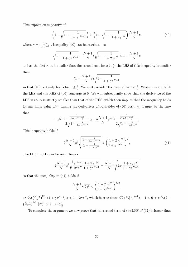
This expression is positive if(1−
√1− 1
1 + γzN−1
)>
(1−
√1− 1
1 + 2γzN
)N + 1
Nz, (40)
where γ = λNµN (1−λ) . Inequality (40) can be rewritten as√
1− 11 + γzN−1
− N + 1N
z
√1− 1
1 + 2γzN< 1− N + 1
Nz
and as the first root is smaller than the second root for z ≥ 12 , the LHS of this inequality is smaller
than
(1− N + 1N
z)√
1− 11 + γzN−1
so that (40) certainly holds for z ≥ 12 . We next consider the case when z < 1
2 . When γ →∞, both
the LHS and the RHS of (40) converge to 0. We will subsequently show that the derivative of the
LHS w.r.t. γ is strictly smaller than that of the RHS, which then implies that the inequality holds
for any finite value of γ. Taking the derivatives of both sides of (40) w.r.t. γ, it must be the case
that
−zN−1
1
(1+γzN−1)2
2√
1− 11+γzN−1
< −2N + 1
NzN+1
1
(1+2γzN )2
2√
1− 11+2γzN
.
This inequality holds if
2N + 1
Nz2
√√√√1− 11+γzN−1
1− 11+2γzN
<
(1 + 2γzN
1 + γzN−1
)2
, (41)
The LHS of (41) can be rewritten as
2N + 1
Nz2
√γzN−1
2γzN
1 + 2γzN
1 + γzN−1=
N + 1N
√2z3
1 + 2γzN
1 + γzN−1
so that the inequality in (41) holds if
N + 1N
√2z3 <
(1 + 2γzN
1 + γzN−1
)3/2
,
or 3√
2(
N+1N
)2/3 (1 + γzN−1)z < 1 + 2γzN , which is true since 3
√2(
N+1N
)2/3z − 1 < 0 < zNγ(2 −(
N+1N
)2/3 3√
2) for all z < 12 .
To complete the argument we now prove that the second term of the LHS of (37) is larger than
30

the second terms of its RHS, i.e.,∫ pm
p(N)R(p)dFN (p) >
∫ pm
p(N+1)R(p)dFN+1(p).
This can be written as
N
∫ pm
p(N)R(p)(1− F (p))N−1dF (p) > (N + 1)
∫ pm
p(N+1)R(p)(1− F (p))NdF (p). (42)
Using the variable change z = 1− F (p), we can rewrite (42) as
∫ 1
0
NR(pm)1 + γzN−1
zN−1dz −∫ 1
0
(N + 1)R(pm)1 + 2γzN−1
zNdz
= R(pm)∫ 1
0zN−1 N
(1 + 2γzN−1
)− (N + 1)z
(1 + γzN−1
)(1 + γzN−1) (1 + 2γzN−1)
dz
= R(pm)∫ 1
0
[NzN−1 − (N + 1)zN
(1 + γzN−1) (1 + 2γzN−1)+
γz2N−1 (2N − (N + 1))(1 + γzN−1) (1 + 2γzN−1)
]dz > 0
The last integral in this expression is certainly larger than∫ 1
0
NzN−1 − (N + 1)zN
(1 + γzN−1) (1 + 2γzN−1)dz
=∫ N
N+1
0
NzN−1 − (N + 1)zN
(1 + γzN−1) (1 + 2γzN−1)dz +
∫ 1
NN+1
NzN−1 − (N + 1)zN
(1 + γzN−1) (1 + 2γzN−1)dz
>
∫ NN+1
0
NzN−1 − (N + 1)zN(1 + γ
[N
N+1
]N−1)(
1 + 2γ[
NN+1
]N−1)dz +
∫ 1
NN+1
NzN−1 − (N + 1)zN(1 + γ
[N
N+1
]N−1)(
1 + 2γ[
NN+1
]N−1)dz
=∫ 1
0
NzN−1 − (N + 1)zN(1 + γ
[N
N+1
]N−1)(
1 + 2γ[
NN+1
]N−1)dz = 0.
The proof is now complete. �
Proof of Proposition 6. Expected total welfare when there are N firms in the market can be
written as
TS(N) = µN (1− λ)∫
R(p)dF (p) + λa2
2b− λ
a
2
∫pdFmin N (p) +
λ
2
∫R(p)dFmin N (p),
which using the variable change z = 1− F (p) can be rewritten as
λa2
4b
2 +
1∫0
[1
γN (1 + γNNzN−1)−(
1−√
1− 11 + γNNzN−1
)NzN−1 +
12
NzN−1
1 + γNNzN−1
]dz
,
31

where γN = λ/µN (1−λ). We need to show that TS(N) > TS(N +1) when λ (or equivalently γN )
is small. Using the fact that 2N/µN < (N + 1)/µN+1 this is certainly the case if
1∫0
γ2N (N − 1)N2z2N−1 + γNNzN−1((3N − 1)z − 1) + (N − 1)
2γNN(1 + γNNzN−1)(1 + 2γNNzN )dz
>
∫ 1
0
N + 1N
z
√2γNNzN
1 + 2γNNzN−
√γNNzN−1
1 + γNNzN−1
NzN−1dz
which is clearly true for γN close to zero. �
References
[1] Anderson, Simon P. and Regis Renault: “Pricing, Product Diversity, and Search Costs: a
Bertrand-Chamberlin-Diamond Model,” RAND Journal of Economics 30, 719-35, 1999.
[2] Baye, Michael R., Kovenock, Dan and Casper de Vries: “It Takes Two to Tango: Equilibria
in a Model of Sales,” Games and Economic Behavior, 4, 493-510, 1992.
[3] Burdett, Kenneth and Kenneth L. Judd: “Equilibrium Price Dispersion,” Econometrica 51-4,
955-69, 1983.
[4] Deneckere, R. and C. Davidson. Incentives to Form Coalitions with bertrand Competition.
Rand Journal of Economics 16, 473-86, 1985.
[5] Hong, Han and Matthew Shum: “Using Price Distributions to Estimate Search Costs,” Rand
Journal of Economics 37, 257-75, 2006.
[6] Hortacsu, Ali and Chad Syverson: “Product Differentiation, Search Costs, and Competition
in the Mutual Fund Industry: a Case Study of S&P 500 Index Funds,” The Quarterly Journal
of Economics 119, 403-56, 2004.
[7] Marc Ivaldi, Bruno Jullien, Patrick Rey, Paul Seabright and Jean Tirole: “The Economics of
Unilateral Effects,” Discussion Paper, DG Competition, European Commission, (2003a).
[8] Janssen, Maarten C. W. and Jose Luis Moraga-Gonzalez: “Strategic Pricing, Consumer Search
and the Number of Firms,” Review of Economic Studies 71, 1089-118, 2004.
32

[9] Janssen, Maarten C. W., Jose Luis Moraga-Gonzalez and Matthijs Wildenbeest: “Truly Costly
Sequential Search and Oligopolistic Pricing,” International Journal of Industrial Organization
23, 451-466, 2005.
[10] Johnson, Eric J., Wendy W. Moe, Peter S. Fader, Steven Bellman and Gerald L. Lohse: “On
the Depth and Dynamics of On-line Search Behavior,” Management Science 50, 299-308, 2004.
[11] Lach, Saul: “Existence and Persistence of Price Dispersion: An Empirical Analysis,” Review
of Economics and Statistics 84, 433-44, 2002.
[12] McAfee, R. Preston: “Multiproduct Equilibrium Price Dispersion,” Journal of Economic The-
ory 67-1, 83-105, 1995.
[13] Moraga-Gonzalez, Jose Luis and Matthijs R. Wildenbeest: “Maximum Likelihood Estima-
tion of Search Costs,” Tinbergen Institute Discussion Paper TI 2006-019/1, The Netherlands,
January 2006.
[14] Perry, Martin K. and Robert H. Porter: “Oligopoly and the Incentives for Horizontal Merger,”
American Economic Review 75, 219-27, 1985.
[15] Pratt, John W., David A. Wise and Richard J. Zeckhauser: “Price Differences in Almost
Competitive Markets,” Quarterly Journal of Economics 93, 189-211, 1979.
[16] Reinganum, Jennifer F.: “A Simple Model of Equilibrium Price Dispersion,” Journal of Polit-
ical Economy 87, 851-858, 1979.
[17] Stigler, George: “The Economics of Information,” Journal of Political Economy 69, 213-25,
1961.
[18] Salant, Stephen W., Sheldon Switzer and Robert J. Reynolds: “Losses from Horizontal Merg-
ers: The Effects of Exogenous Change in Industry Structure on Cournot-Nash Equililibrium.
Quarterly Journal of Economics 98: 185-99, 1983
[19] Sorensen, Alan T.: “An Empirical Model of Heterogeneous Consumer Search for Retail Pre-
scription Drugs,” NBER Working Paper No. 8548, 2001.
[20] Stahl, Dale O.: “Oligopolistic Pricing with Sequential Consumer Search,” American Economic
Review 79-4, 700-12, 1989.
33
[21] Stahl, Dale O.: “Oligopolistic Pricing with Heterogeneous Consumer Search,” International
Journal of Industrial Organization 14, 243-268, 1996.
[22] Williamson, O.: “Economies as an Antitrust Defense: the Welfare Trade-Offs,” American
Economic Review 58, 18-36, 1968.
34