vol. 172, no. 1 the american naturalist july 2008 �

On Net Reproductive Rate and the Timing of

Reproductive Output

T. de-Camino-Beck1,* and M. A. Lewis1,2,†

1. Department of Mathematical and Statistical Sciences, Universityof Alberta, Edmonton, Alberta T6G 2G1, Canada;2. Department of Biological Sciences, University of Alberta,Edmonton, Alberta T6G 2G1, Canada

Submitted January 30, 2007; Accepted February 5, 2008;Electronically published May 28, 2008

Online enhancement: appendix.

abstract: Understanding the relationship between life-history pat-terns and population growth is central to demographic studies. Herewe derive a new method for calculating the timing of reproductiveoutput, from which the generation time and its variance can also becalculated. The method is based on the explicit computation of thenet reproductive rate ( ) using a new graphical approach. UsingR 0

nodding thistle, desert tortoise, creeping aven, and cat’s ear as ex-amples, we show how and the timing of reproduction is calculatedR 0

and interpreted, even in cases with complex life cycles. We show thatthe explicit formula allows us to explore the effect of all repro-R 0

ductive pathways in the life cycle, something that cannot be donewith traditional analysis of the population growth rate (l). Addi-tionally, we compare a recently published method for determiningpopulation persistence conditions with the condition andR 1 10

show how the latter is simpler and more easily interpreted biolog-ically. Using our calculation of the timing of reproductive output,we illustrate how this demographic measure can be used to under-stand the effects of life-history traits on population growth andcontrol.

Keywords: matrix model, net reproductive rate, biological control,generation time, reproductive output, persistence.

Persistence of biological populations is the result of theevolution of life-history patterns that have consequencesfor population growth. Early theoretical work by Cole

* E-mail: tomasd@math.ualberta.ca.

† E-mail: mlewis@math.ualberta.ca.

Am. Nat. 2008. Vol. 172, pp. 128–139. � 2008 by The University of Chicago.0003-0147/2008/17201-42375$15.00. All rights reserved.DOI: 10.1086/588060

(1954) showed how changes in reproductive schedules canhave consequences in population growth rate. Cole’s workestablished the foundations of demographic analysis—based on the estimation of parameters such as growth rate,net reproductive rate, and length of a generation—andprovided the foundation for theoretical and empiricalwork on population demography (e.g., Cole 1960; Mur-doch 1966; Charnov and Schaffer 1973; Goodman 1975).Since Cole’s work, substantial theoretical advances havebeen achieved, in particular with the use of matrix modelspopularized and summarized in a book by Caswell (2001).

Matrix models provide an intuitive modeling strategywhere the life cycle of the organisms can be described ex-plicitly in terms of life ages or stages. Demographic param-eters of population growth rate (l), net reproductive rate(the lifetime reproductive output of an individual; ), andR 0

generation time (the time it takes for the population toincrease by ) have also been derived for matrix modelsR 0

(Caswell 2001), providing a direct connection between lifecycle structure and these demographic parameters.

In general, most of the analysis in matrix models hasbeen based on the numerical calculation of l and thesensitivity of l to model parameters. In particular, elas-ticity or sensitivity analysis of l to age/stage transitions inmatrix models has become a standard method in demo-graphic analysis in ecology, management, and evolution(Silvertown et al. 1993; Franco and Silvertown 1996; Pfister1998; Oli and Dobson 2003, 2005; Gaillard et al. 2005;Shea 2004). In all but the simplest matrix models, cal-culation of the population growth rate and elasticity re-quires numerical estimates, thus restricting results to theparticular population parameter estimates.

Although total reproductive output and timing of re-production have an impact on population growth andpersistence, parameters like and generation time haveR 0

not been well studied using matrix models. The calculationof is thought to be too complicated to perform ana-R 0

lytically (Hastings and Botsford 2006b), and its numericalcalculation for stage-structured models (Cushing andZhou 1994) has rarely been made, in favor of the calcu-lation of l and elasticity/sensitivity analysis of l. The dif-

Reproductive Rate and Reproductive Output 129

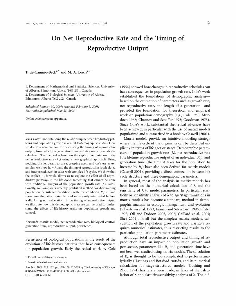
Figure 1: Simple matrix and its associated graph. There is a2 # 2 Adirected edge in the graph for every entry in the matrix. In the graph,aij

for a transition , the edge is directed from node j to node i.aij

ficult calculation of generation time in stage-structuredmodels (Cochran and Ellner 1992; Lebreton 2005) haddissuaded demographers from using as a measure ofR 0

the impacts of reproduction and survival on populationgrowth and persistence, primarily because the interpre-tation of without an estimate of generation time canR 0

be misleading (Birch 1948; Cole 1960; Caswell 2001). Herewe show that both and mean generation time can beR 0

directly calculated for stage-structured models.In a previous article (de-Camino-Beck and Lewis 2007),

we developed a graphical method for calculating ex-R 0

plicitly, and we showed how it can be applied in the contextof biological control. In this article, we derive a formulafor calculating the timing of reproductive output based onthe equation. This formula allows for the calculationR 0

of the timing of reproductive output, the mean generationtime, and the mean generation time variance for stage-structured models. We start by giving the theoretical back-ground in matrix models and life cycle graphs. Then, webriefly describe the graph-theoretic method to calculate

and the timing of reproductive output. Later, we showR 0

with four examples how and timing of reproductiveR 0

output are calculated, and we discuss the implications fordemographic analysis. Additionally, we compare the con-dition with a persistence condition for matrix mod-R 1 10

els derived by DeAngelis et al. (1986) and recently re-derived by Hastings and Botsford (2006b), and we discussits implication in the management and control oforganisms.

Net Reproductive Rate, Generation Time,and Persistence

In this section, we briefly introduce matrix models. First,we show how to calculate the net reproductive rate usinga graphical approach. Next, we show that the concept ofthe net reproductive rate can be extended to determine

not only the total number of offspring produced but alsotheir distribution over the life span of the parent. Then,we describe the persistence condition proposed by De-Angelis et al. (1986) and Hastings and Botsford (2006b),which we will call the Hastings-Botsford persistence con-dition, and compare this with .R 1 10

Matrix Models

Stage-structured models are population dynamics modelswhere life cycle stages are explicitly defined. Stages can besize classes or life forms (e.g., larvae, juvenile, seeds, seed-ling, adult plants). In matrix form, a stage-structuredmodel is defined as

n p An , (1)t�1 t

where is a vector of stages at time t and is ann A n # nt

projection matrix. Each entry, , in the matrix representsa Aij

the contribution from stage j in time t to stage i in time. The projection matrix can also be represented ast � 1 A

a life cycle graph where each node in the graph correspondsto a stage and each arrow represents transitions, (fig. 1).aij

The matrix is composed of survivorship and fecundityAtransitions. These can be decomposed into a transitionmatrix and a fecundity matrix . Transition matrix en-T Ftries, , describe survivorship, the probability of survivaltij

from stage j to i. The fecundity matrix entries, , describefij

fecundities, the maximum reproductive output from stagej to i. This decomposition is not mathematically uniquebut is uniquely determined by the biology of the organism.

Net Reproductive Rate R0

Given an initial distribution of stages , the number ofn 0

offspring produced by the individuals initially present is

2 2… …Fn � FTn � FT n � p F(I � T � T � )n0 0 0 0

�1p F(I � T) n .0

(2)

The first term on the left-hand side of the first line of theequation represents first-year fecundity, the second termrepresents fecundity following a year of survival, and thethird term represents fecundity following two years of sur-vival and so forth. The matrix is referred to as�1F(I � T)the next-generation matrix (Cushing and Zhou 1994; Liand Schneider 2002).

The net reproductive rate, , is the average number ofR 0

offspring that a single reproducing individual can produce

130 The American Naturalist

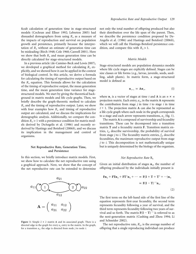
Figure 2: A shows the transition matrix and its decomposition in sur-vivorship and fecundities. In B, fecundities are multiplied by . Then,�1R0

using rule A in figure 3, self-loops (gray) are eliminated, yielding thegraph in C. Node 1 is eliminated by multiplying the two edges in gray(rule in fig. 3C to produce the graph in D). The resulting loops are addedtogether (rule in fig. 3B to obtain E). Applying step 5 in E to the singlenode graph yields .R0

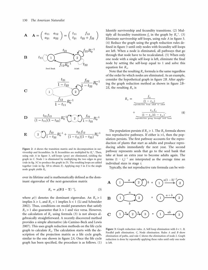
Figure 3: Graph reduction rules. A, Self-loop elimination with . B,b ! 1Parallel path elimination. C, Node elimination. Rules A and B showelimination of paths, and rule C shows the elimination of node 2. Graphreduction is done by repeatedly applying these rules until only one nodeis left.

over its lifetime and is mathematically defined as the dom-inant eigenvalue of the next-generation matrix

�1R p r[F(I � T) ], (3)0

where denotes the dominant eigenvalue. Anr(7) R 1 10

implies , and implies (Li and Schneiderl 1 1 R ! 1 l ! 10

2002). Thus, conditions on model parameters that satisfyalso guarantee that and vice versa. However,R 1 1 l 1 10

the calculation of using formula (3) is not always al-R 0

gebraically straightforward. A recently discovered methodprovides a simple alternative (de-Camino-Beck and Lewis2007). This uses graph reduction methods on the life cyclegraph to calculate . The calculation starts with the de-R 0

scription of the projection matrix as a life cycle graph,similar to the one shown in figure 2A. Once the life cyclegraph has been specified, the procedure is as follows. (1)

Identify survivorship and fecundity transitions. (2) Mul-tiply all fecundity transitions in the graph by . (3)�1f Rij 0

Eliminate survivorship self-loops, using rule A in figure 3.(4) Reduce the graph using the graph reduction rules de-fined in figure 3 until only nodes with fecundity self-loopsare left. When a node is eliminated, all pathways that gothrough that node have to be recalculated. (5) When onlyone node with a single self-loop is left, eliminate the finalnode by setting the self-loop equal to 1 and solve thisequation for .R 0

Note that the resulting formula is the same regardlessR 0

of the order by which nodes are eliminated. As an example,consider the hypothetical graph in figure 2B. After apply-ing the graph reduction method as shown in figure 2B–2E, the resulting isR 0

f22R p0 (1 � t )\22reproduction from adult to adult

t f21 12� . (4)(1 � t )(1 � t )\11 22

reproduction going through seed bank

The population persists if . The formula showsR 1 1 R0 0

two reproductive pathways. If either is 11, then the pop-ulation persists. The first pathway accounts for the repro-duction of plants that start as adults and produce repro-ducing adults immediately the next year. The secondpathway represents seeds that go to the seed bank thattake at least an extra year to become adults again. Theterms are interpreted as the average time an�1(1 � t )ii

individual stays in stage i.Typically, the net reproductive rate formula can be writ-

Reproductive Rate and Reproductive Output 131

ten explicitly as the sum of fecundities for m pathways asfollows:

…R p R � R � � R , (5)0 1 2 m

where is the fecundity for a pathway that ends in re-Ri

production. We will call each a fecundity pathway. Be-Ri

cause the pathways are summed, the population will persistif any . From the previous example, the first pathwayR 1 1i

is , and the second isR p f /(1 � t ) R p t f /[(1 �1 22 22 2 21 12

. If , , or the sum is 11, then thet )(1 � t )] R R R � R11 22 1 2 1 2

population will persist.This graph reduction method for calculating (de-R 0

Camino-Beck and Lewis 2007) relates to a different es-tablished method for calculating the eigenvalues l of theprojection matrix . There, each entry of the life cycleA aij

graph is multiplied by , and the graph reduction steps�1l

of figure 3 are used to yield a characteristic polynomialfor the eigenvalues l (Caswell 2001). The difference be-tween the methods (multiplying by [step 2] rather�1f Rij 0

than multiplying each by [above]) is suf-�1a p t � f lij ij ij

ficient to yield the reproductive rate rather than l. InR 0

other words, is the dominant eigenvalue of the next-R 0

generation matrix , while l is the dominant�1F(I � T)eigenvalue of the projection matrix (Caswell 2001).T � FThe population growth rate, l, can be calculated with thegraph method as well. However, the procedure yields ahigher-degree polynomial where the interpretation is notintuitive. For example, the characteristic polynomial forthe eigenvalues associated with the life cycle graph in figure2 is

2l � (t � t � f )l � [t (t � f ) � t f ] p 0, (6)11 22 22 11 22 22 21 12

which has dominant eigenvalue

12�l p t � t � f � (t � t � f ) � 4[t (t � f ) � t f ] .11 22 22 11 22 22 11 22 22 21 12{ }2

(7)

While this eigenvalue gives the population persistencecondition as , there is no intuitive interpretation ofl 1 1the condition, unlike the fecundity pathways used for

. When the number of stages in the life cycle is threeR 0

or more, it is difficult or impossible to calculate the dom-inant eigenvalue explicitly, and numerical methods mustinstead be used.

Timing of Reproductive Output

Since the work by Cole (1954), timing of reproductiveoutput and its implications for fitness have been the sub-

ject of widespread study (Beckerman et al. 2002; Ranta etal. 2002; Oli and Dobson 2003; Coulson et al. 2006). Inthis section, we show our calculation of how can beR 0

extended to yield the total number of offspring producedas well as their distribution over the life span of the parent.To explore timing of reproduction in a stage-structuredmodel using , the time that it takes to go through eachR 0

pathway has to be included in the formula. Rather thanR 0

grouping terms according to fecundity pathway terms,equation (5), in the net reproductive rate, formula can begrouped according to the number of time steps taken tocomplete a pathway. For example, equation (4) can berewritten as

2 …R p f (1 � t � t � )0 22 22 22

2 2… …� t f (1 � t � t � )(1 � t � t � ) (8)21 12 11 11 22 22

p f22\one time step to reproduction

� (f t � t f ) (9)22 22 21 12\two time steps to reproduction

2 …� (f t � t f t � t f t ) �22 22 21 12 11 21 12 22\three time steps to reproduction

…p S � S � S � . (10)1 2 3

If the population is growing ( ), offspring producedl 1 1after several time steps will contribute less to populationgrowth than those produced immediately. This motivatesus to connect to l by using the current value of futureR 0

reproduction. The current value of future reproductiveoutput is assigned on the basis of the contribution thatthe future reproductive output will make to the overallpopulation growth. Formally, we define and start�1t p l

by multiplying each pathway that takes n time steps tocomplete by the weight . From the example above, path-nt

way takes two time steps to completeS p (f t � t f )2 22 22 21 12

( ); thus, the pathways with its associated weights aren p 2. Thus, means , and2 2S t p (f t � t f )t l 1 1 t ! 12 22 22 21 12

the reproductive output two steps hence is diminished bythe factor . Summing across all possible values of n yields2t

the present value of all future reproduction

�

nS(t) p S t . (11)� nnp1

By analogy with generating functions in probability the-ory, we also refer to this as the -generating function.R 0

Equation (11) can also be found by taking the z transformof the life cycle graph with . For details of applying�1z p t

132 The American Naturalist

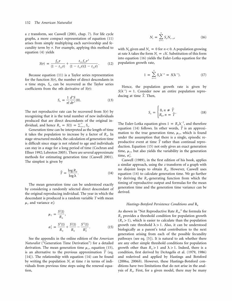
a z transform, see Caswell (2001, chap. 7). For life cyclegraphs, a more compact representation of equation (11)arises from simply multiplying each survivorship and fe-cundity term by t. For example, applying this method toequation (4) yields

2f t t f t22 21 12S(t) p � . (12)(1 � t t) (1 � t t)(1 � t t)22 11 22

Because equation (11) is a Taylor series representationfor the function , the number of direct descendants inS(t)n time steps, , can be recovered as the Taylor seriesSn

coefficients from the nth derivative of :S(t)

n1 d SS p (0). (13)n nn! dt

The net reproductive rate can be recovered from byS(t)recognizing that it is the total number of new individualsproduced that are direct descendants of the original in-dividual, and hence

�R p S(1) p � S .0 nnp1

Generation time can be interpreted as the length of timeit takes the population to increase by a factor of . InR 0

stage-structured models, the calculation of generation timeis difficult since stage is not related to age and individualscan stay in a stage for a long period of time (Cochran andEllner 1992; Lebreton 2005). There are several approximatemethods for estimating generation time (Caswell 2001).The simplest is given by

log R 0T̃ p . (14)log l

The mean generation time can be understood exactlyby considering a randomly selected direct descendant ofthe original reproducing individual. The year in which thedescendant is produced is a random variable T with mean

and variance :2m jT T

′S (1)m p ,T R 0

′′ ′ ′2S (1) S (1) S (1)2j p � � . (15)T 2R R R0 0 0

See the appendix in the online edition of the AmericanNaturalist (“Generation Time Derivation”) for a detailedderivation. The mean generation time , equation (15),mT

is an alternative to the previous approximation (eq.T̃[14]). The relationship with equation (14) can be foundby writing the population at time t in terms of indi-Nt

viduals from previous time steps using the renewal equa-tion,

�

N p S N , (16)�t n t�nnp1

with given and for . A population growingN N p 0 n ! 00 n

at rate l takes the form . Substitution of this formtN p clt

into equation (16) yields the Euler-Lotka equation for thepopulation growth rate,

�

�n �11 p S l p S(l ). (17)� nnp1

Hence, the population growth rate is given by. Consider now an entire population repro-�1S(l ) p 1

ducing at time . Then,T̃

˜0, n ( TS p . (18)n ˜{R , n p T0

The Euler-Lotka equation gives , and therefore˜�T1 p R l0

equation (14) follows. In other words, is an approxi-T̃mation to the true generation time, , which is foundmT

under the assumption that there is a single, episodic re-productive event at time rather than continual repro-T̃duction. Equation (15) not only gives an exact generationtime, , but also yields the variability in the generationmT

time, .2jT

Caswell (1989), in the first edition of his book, appliesa similar approach, using the z transform of a graph withno disjoint loops to obtain . However, Caswell usesR 0

equation (14) to calculate generation time. We go furtherby deriving the -generating function from which theR 0

timing of reproductive output and formulas for the meangeneration time and the generation time variance can bederived.

Hastings-Botsford Persistence Conditions and R0

As shown in “Net Reproductive Rate ,” the formula forR 0

provides a threshold condition for population growthR 0

( ), which is easier to calculate than the populationR 1 10

growth rate threshold . Also, it can be understoodl 1 1biologically as a parent’s total contribution to the nextgeneration arising from each of the possible fecunditypathways (see eq. [5]). It is natural to ask whether thereare any other simple threshold conditions for populationgrowth other than and . Indeed, there is aR 1 1 l 1 10

condition, first derived by DeAngelis et al. (1979, 1986)and rederived and applied by Hastings and Botsford(2006a, 2006b). However, these Hastings-Botsford con-ditions have two limitations that do not arise in the anal-ysis of . First, for a given model, there may be manyR 0

Reproductive Rate and Reproductive Output 133

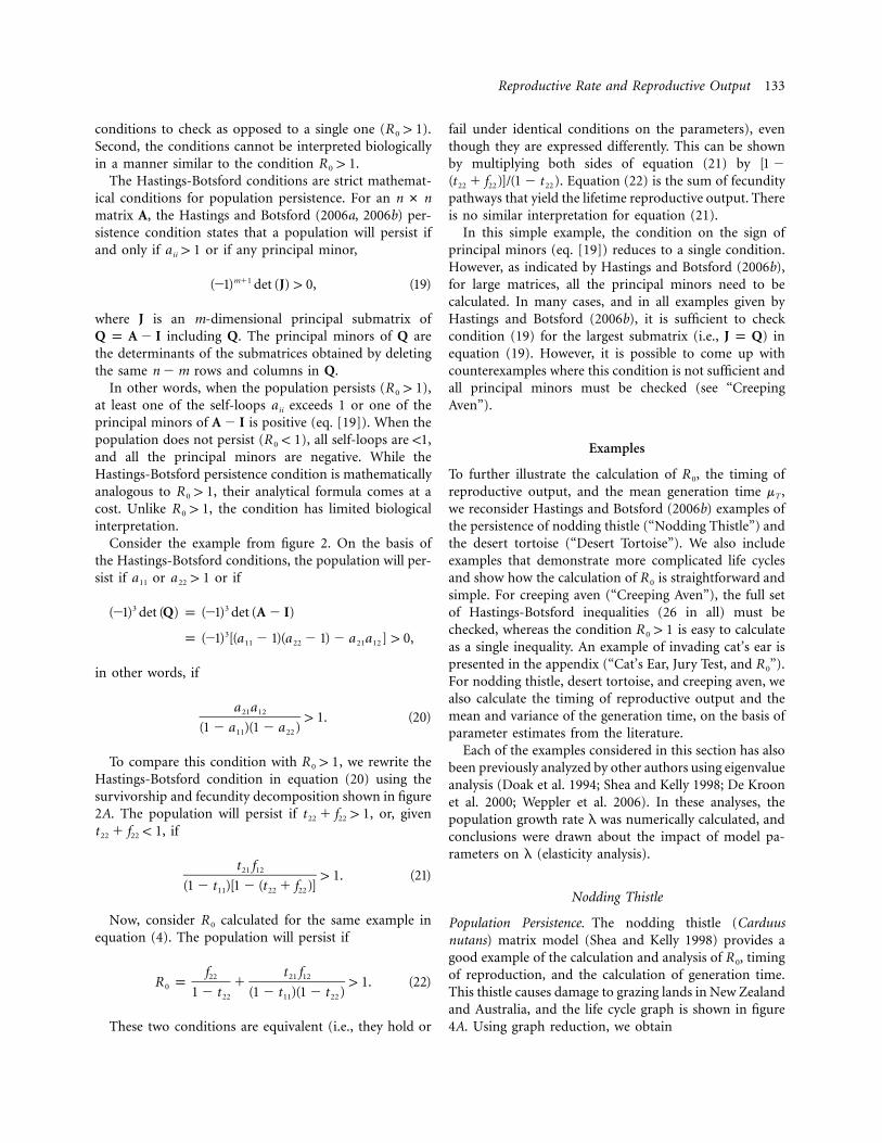
conditions to check as opposed to a single one ( ).R 1 10

Second, the conditions cannot be interpreted biologicallyin a manner similar to the condition .R 1 10

The Hastings-Botsford conditions are strict mathemat-ical conditions for population persistence. For an n # nmatrix , the Hastings and Botsford (2006a, 2006b) per-Asistence condition states that a population will persist ifand only if or if any principal minor,a 1 1ii

m�1(�1) det (J) 1 0, (19)

where is an m-dimensional principal submatrix ofJincluding . The principal minors of areQ p A � I Q Q

the determinants of the submatrices obtained by deletingthe same rows and columns in .n � m Q

In other words, when the population persists ( ),R 1 10

at least one of the self-loops exceeds 1 or one of theaii

principal minors of is positive (eq. [19]). When theA � Ipopulation does not persist ( ), all self-loops are !1,R ! 10

and all the principal minors are negative. While theHastings-Botsford persistence condition is mathematicallyanalogous to , their analytical formula comes at aR 1 10

cost. Unlike , the condition has limited biologicalR 1 10

interpretation.Consider the example from figure 2. On the basis of

the Hastings-Botsford conditions, the population will per-sist if or or ifa a 1 111 22

3 3(�1) det (Q) p (�1) det (A � I)

3p (�1) [(a � 1)(a � 1) � a a ] 1 0,11 22 21 12

in other words, if

a a21 121 1. (20)

(1 � a )(1 � a )11 22

To compare this condition with , we rewrite theR 1 10

Hastings-Botsford condition in equation (20) using thesurvivorship and fecundity decomposition shown in figure2A. The population will persist if , or, givent � f 1 122 22

, ift � f ! 122 22

t f21 121 1. (21)

(1 � t )[1 � (t � f )]11 22 22

Now, consider calculated for the same example inR 0

equation (4). The population will persist if

f t f22 21 12R p � 1 1. (22)0 1 � t (1 � t )(1 � t )22 11 22

These two conditions are equivalent (i.e., they hold or

fail under identical conditions on the parameters), eventhough they are expressed differently. This can be shownby multiplying both sides of equation (21) by [1 �

. Equation (22) is the sum of fecundity(t � f )]/(1 � t )22 22 22

pathways that yield the lifetime reproductive output. Thereis no similar interpretation for equation (21).

In this simple example, the condition on the sign ofprincipal minors (eq. [19]) reduces to a single condition.However, as indicated by Hastings and Botsford (2006b),for large matrices, all the principal minors need to becalculated. In many cases, and in all examples given byHastings and Botsford (2006b), it is sufficient to checkcondition (19) for the largest submatrix (i.e., ) inJ p Qequation (19). However, it is possible to come up withcounterexamples where this condition is not sufficient andall principal minors must be checked (see “CreepingAven”).

Examples

To further illustrate the calculation of , the timing ofR 0

reproductive output, and the mean generation time ,mT

we reconsider Hastings and Botsford (2006b) examples ofthe persistence of nodding thistle (“Nodding Thistle”) andthe desert tortoise (“Desert Tortoise”). We also includeexamples that demonstrate more complicated life cyclesand show how the calculation of is straightforward andR 0

simple. For creeping aven (“Creeping Aven”), the full setof Hastings-Botsford inequalities (26 in all) must bechecked, whereas the condition is easy to calculateR 1 10

as a single inequality. An example of invading cat’s ear ispresented in the appendix (“Cat’s Ear, Jury Test, and ”).R 0

For nodding thistle, desert tortoise, and creeping aven, wealso calculate the timing of reproductive output and themean and variance of the generation time, on the basis ofparameter estimates from the literature.

Each of the examples considered in this section has alsobeen previously analyzed by other authors using eigenvalueanalysis (Doak et al. 1994; Shea and Kelly 1998; De Kroonet al. 2000; Weppler et al. 2006). In these analyses, thepopulation growth rate l was numerically calculated, andconclusions were drawn about the impact of model pa-rameters on l (elasticity analysis).

Nodding Thistle

Population Persistence. The nodding thistle (Carduusnutans) matrix model (Shea and Kelly 1998) provides agood example of the calculation and analysis of , timingR 0

of reproduction, and the calculation of generation time.This thistle causes damage to grazing lands in New Zealandand Australia, and the life cycle graph is shown in figure4A. Using graph reduction, we obtain

134 The American Naturalist

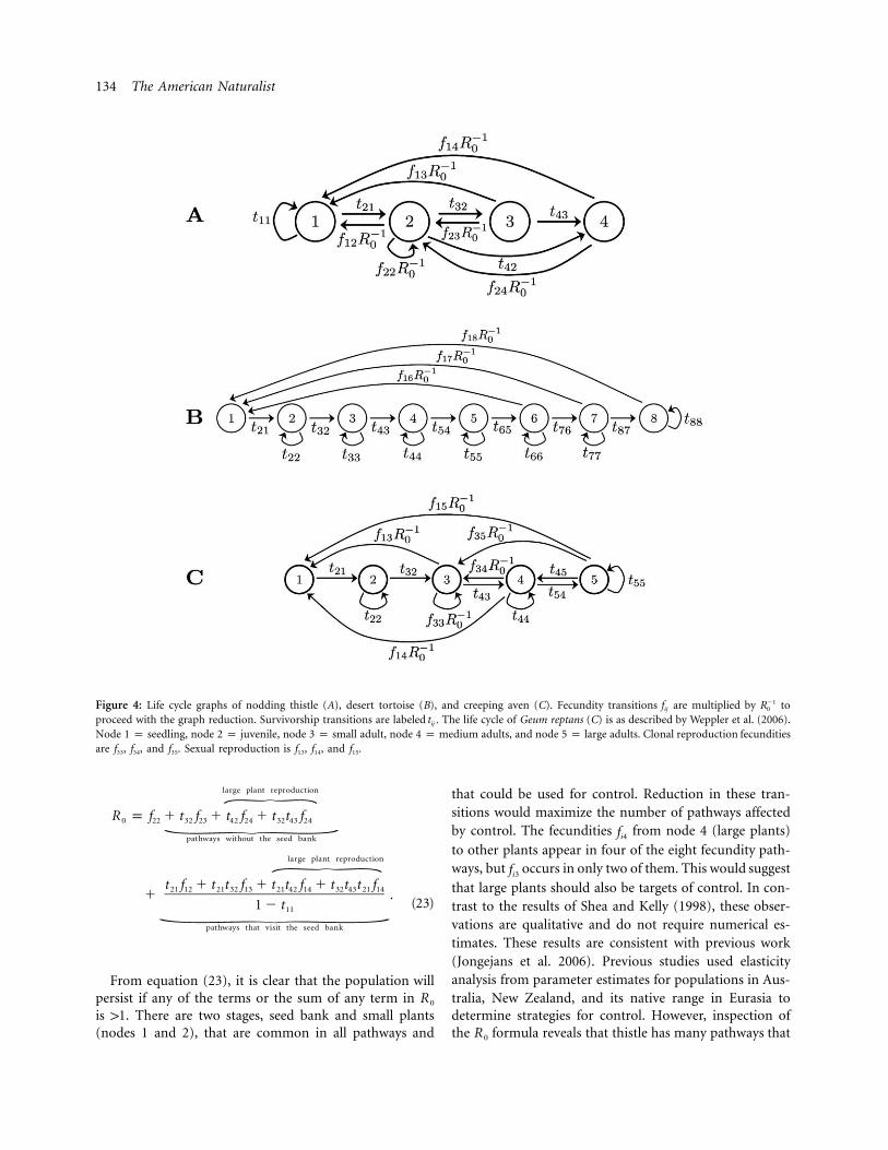
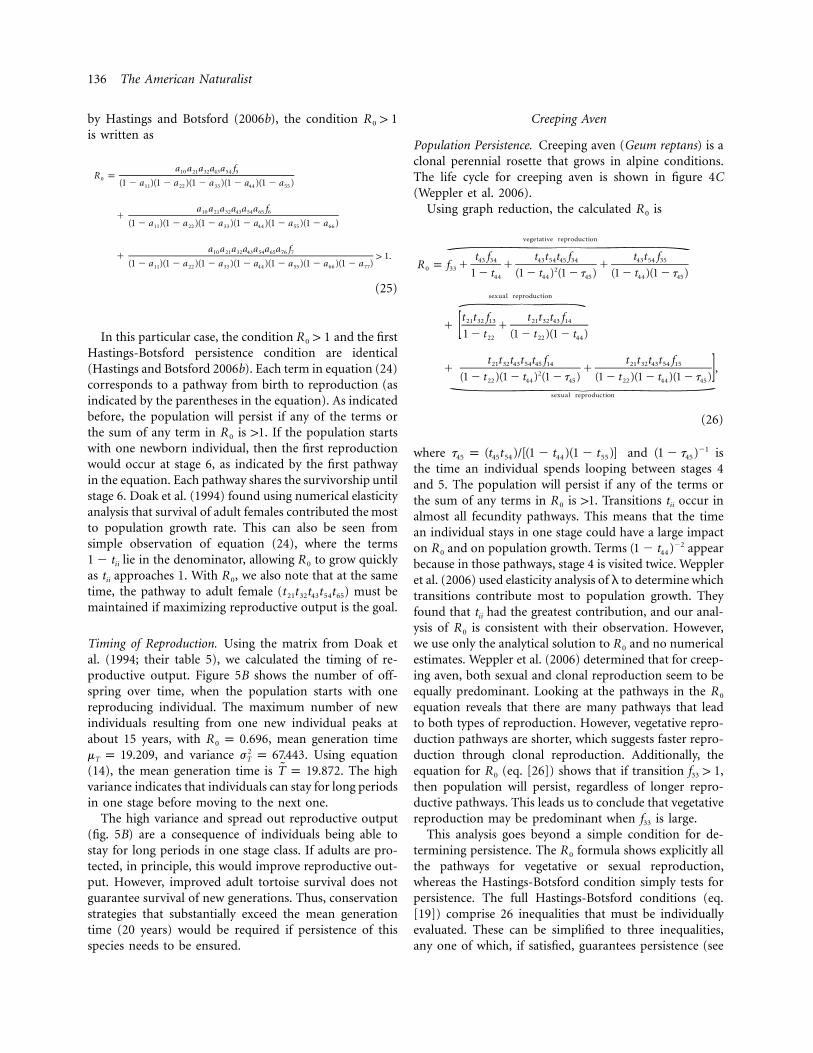
Figure 4: Life cycle graphs of nodding thistle (A), desert tortoise (B), and creeping aven (C). Fecundity transitions are multiplied by to�1f Rij 0

proceed with the graph reduction. Survivorship transitions are labeled . The life cycle of Geum reptans (C) is as described by Weppler et al. (2006).tij

Node 1 p seedling, node 2 p juvenile, node 3 p small adult, node 4 p medium adults, and node 5 p large adults. Clonal reproduction fecunditiesare f33, f34, and f35. Sexual reproduction is f13, f14, and f15.

large plant reproduction=R p f � t f � t f � t t f0 22 32 23 42 24 32 43 24\

pathways without the seed bank

large plant reproduction=t f � t t f � t t f � t t t f21 12 21 32 13 21 42 14 32 43 21 14� .

1 � t11(23)\

pathways that visit the seed bank

From equation (23), it is clear that the population willpersist if any of the terms or the sum of any term in R 0

is 11. There are two stages, seed bank and small plants(nodes 1 and 2), that are common in all pathways and

that could be used for control. Reduction in these tran-sitions would maximize the number of pathways affectedby control. The fecundities from node 4 (large plants)fi4

to other plants appear in four of the eight fecundity path-ways, but occurs in only two of them. This would suggestfi3

that large plants should also be targets of control. In con-trast to the results of Shea and Kelly (1998), these obser-vations are qualitative and do not require numerical es-timates. These results are consistent with previous work(Jongejans et al. 2006). Previous studies used elasticityanalysis from parameter estimates for populations in Aus-tralia, New Zealand, and its native range in Eurasia todetermine strategies for control. However, inspection ofthe formula reveals that thistle has many pathways thatR 0

Reproductive Rate and Reproductive Output 135

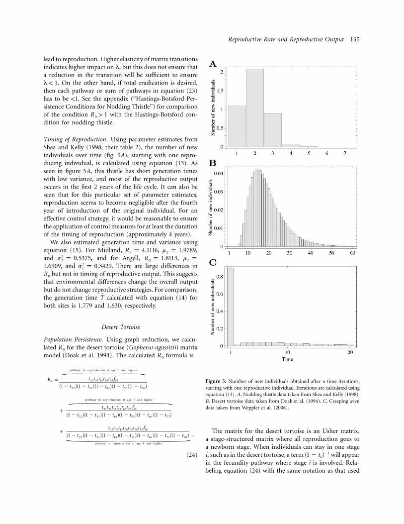
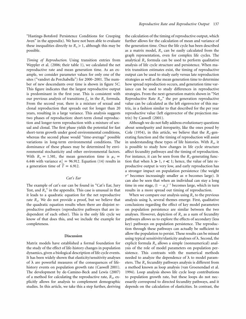
Figure 5: Number of new individuals obtained after n time iterations,starting with one reproductive individual. Iterations are calculated usingequation (13). A, Nodding thistle data taken from Shea and Kelly (1998).B, Desert tortoise data taken from Doak et al. (1994). C, Creeping avendata taken from Weppler et al. (2006).

lead to reproduction. Higher elasticity of matrix transitionsindicates higher impact on l, but this does not ensure thata reduction in the transition will be sufficient to ensure

. On the other hand, if total eradication is desired,l ! 1then each pathway or sum of pathways in equation (23)has to be !1. See the appendix (“Hastings-Botsford Per-sistence Conditions for Nodding Thistle”) for comparisonof the condition with the Hastings-Botsford con-R 1 10

dition for nodding thistle.

Timing of Reproduction. Using parameter estimates fromShea and Kelly (1998; their table 2), the number of newindividuals over time (fig. 5A), starting with one repro-ducing individual, is calculated using equation (13). Asseen in figure 5A, this thistle has short generation timeswith low variance, and most of the reproductive outputoccurs in the first 2 years of the life cycle. It can also beseen that for this particular set of parameter estimates,reproduction seems to become negligible after the fourthyear of introduction of the original individual. For aneffective control strategy, it would be reasonable to ensurethe application of control measures for at least the durationof the timing of reproduction (approximately 4 years).

We also estimated generation time and variance usingequation (15). For Midland, , ,R p 4.1116 m p 1.97890 T

and , and for Argyll, ,2j p 0.5375 R p 1.8113 m pT 0 T

, and . There are large differences in21.6909 j p 0.3429T

but not in timing of reproductive output. This suggestsR 0

that environmental differences change the overall outputbut do not change reproductive strategies. For comparison,the generation time calculated with equation (14) forT̃both sites is 1.779 and 1.630, respectively.

Desert Tortoise

Population Persistence. Using graph reduction, we calcu-lated for the desert tortoise (Gopherus agassizii) matrixR 0

model (Doak et al. 1994). The calculated formula isR 0

pathway to reproduction at age 6 and higher=R p0

t t t t t f21 32 43 54 65 16

(1 � t )(1 � t )(1 � t )(1 � t )(1 � t )22 33 44 55 66

pathway to reproduction at age 7 and higher=t t t t t t f21 32 43 54 65 76 17�

(1 � t )(1 � t )(1 � t )(1 � t )(1 � t )(1 � t )22 33 44 55 66 77

t t t t t t t f21 32 43 54 65 76 87 18�(1 � t )(1 � t )(1 � t )(1 � t )(1 � t )(1 � t )(1 � t )22 33 44 55 66 77 88

.\

pathway to reproduction at age 8 and higher

(24)

The matrix for the desert tortoise is an Usher matrix,a stage-structured matrix where all reproduction goes toa newborn stage. When individuals can stay in one stagei, such as in the desert tortoise, a term will appear�1(1 � t )ii

in the fecundity pathway where stage i is involved. Rela-beling equation (24) with the same notation as that used

136 The American Naturalist

by Hastings and Botsford (2006b), the condition R 1 10

is written as

a a a a a f10 21 32 43 54 5R p0(1 � a )(1 � a )(1 � a )(1 � a )(1 � a )11 22 33 44 55

a a a a a a f10 21 32 43 54 65 6�(1 � a )(1 � a )(1 � a )(1 � a )(1 � a )(1 � a )11 22 33 44 55 66

a a a a a a a f10 21 32 43 54 65 76 7� 1 1.(1 � a )(1 � a )(1 � a )(1 � a )(1 � a )(1 � a )(1 � a )11 22 33 44 55 66 77

(25)

In this particular case, the condition and the firstR 1 10

Hastings-Botsford persistence condition are identical(Hastings and Botsford 2006b). Each term in equation (24)corresponds to a pathway from birth to reproduction (asindicated by the parentheses in the equation). As indicatedbefore, the population will persist if any of the terms orthe sum of any term in is 11. If the population startsR 0

with one newborn individual, then the first reproductionwould occur at stage 6, as indicated by the first pathwayin the equation. Each pathway shares the survivorship untilstage 6. Doak et al. (1994) found using numerical elasticityanalysis that survival of adult females contributed the mostto population growth rate. This can also be seen fromsimple observation of equation (24), where the terms

lie in the denominator, allowing to grow quickly1 � t Rii 0

as approaches 1. With , we also note that at the samet Rii 0

time, the pathway to adult female ( ) must bet t t t t21 32 43 54 65

maintained if maximizing reproductive output is the goal.

Timing of Reproduction. Using the matrix from Doak etal. (1994; their table 5), we calculated the timing of re-productive output. Figure 5B shows the number of off-spring over time, when the population starts with onereproducing individual. The maximum number of newindividuals resulting from one new individual peaks atabout 15 years, with , mean generation timeR p 0.6960

, and variance . Using equation2m p 19.209 j p 67.443T T

(14), the mean generation time is . The highT̃ p 19.872variance indicates that individuals can stay for long periodsin one stage before moving to the next one.

The high variance and spread out reproductive output(fig. 5B) are a consequence of individuals being able tostay for long periods in one stage class. If adults are pro-tected, in principle, this would improve reproductive out-put. However, improved adult tortoise survival does notguarantee survival of new generations. Thus, conservationstrategies that substantially exceed the mean generationtime (20 years) would be required if persistence of thisspecies needs to be ensured.

Creeping Aven

Population Persistence. Creeping aven (Geum reptans) is aclonal perennial rosette that grows in alpine conditions.The life cycle for creeping aven is shown in figure 4C(Weppler et al. 2006).

Using graph reduction, the calculated isR 0

vegetative reproduction=t f t t t f t t f43 34 43 54 45 34 43 54 35R p f � � �0 33 21 � t (1 � t ) (1 � t ) (1 � t )(1 � t )44 44 45 44 45

sexual reproduction=t t f t t t f21 32 13 21 32 43 14� �[ 1 � t (1 � t )(1 � t )22 22 44

t t t t t f t t t t f21 32 43 54 45 14 21 32 43 54 15� � ,2 ](1 � t )(1 � t ) (1 � t ) (1 � t )(1 � t )(1 � t )22 44 45 22 44 45\

sexual reproduction

(26)

where and is�1t p (t t )/[(1 � t )(1 � t )] (1 � t )45 45 54 44 55 45

the time an individual spends looping between stages 4and 5. The population will persist if any of the terms orthe sum of any terms in is 11. Transitions occur inR t0 ii

almost all fecundity pathways. This means that the timean individual stays in one stage could have a large impacton and on population growth. Terms appear�2R (1 � t )0 44

because in those pathways, stage 4 is visited twice. Weppleret al. (2006) used elasticity analysis of l to determine whichtransitions contribute most to population growth. Theyfound that had the greatest contribution, and our anal-tii

ysis of is consistent with their observation. However,R 0

we use only the analytical solution to and no numericalR 0

estimates. Weppler et al. (2006) determined that for creep-ing aven, both sexual and clonal reproduction seem to beequally predominant. Looking at the pathways in the R 0

equation reveals that there are many pathways that leadto both types of reproduction. However, vegetative repro-duction pathways are shorter, which suggests faster repro-duction through clonal reproduction. Additionally, theequation for (eq. [26]) shows that if transition ,R f 1 10 33

then population will persist, regardless of longer repro-ductive pathways. This leads us to conclude that vegetativereproduction may be predominant when is large.f33

This analysis goes beyond a simple condition for de-termining persistence. The formula shows explicitly allR 0

the pathways for vegetative or sexual reproduction,whereas the Hastings-Botsford condition simply tests forpersistence. The full Hastings-Botsford conditions (eq.[19]) comprise 26 inequalities that must be individuallyevaluated. These can be simplified to three inequalities,any one of which, if satisfied, guarantees persistence (see

Reproductive Rate and Reproductive Output 137

“Hastings-Botsford Persistence Conditions for CreepingAven” in the appendix). We have not been able to evaluatethese inequalities directly to , although this may beR 1 10

possible.

Timing of Reproduction. Using transition entries fromWeppler et al. (2006; their table 1), we calculated the netreproductive rate and mean generation time. As an ex-ample, we consider parameter values for only one of thesites (“vandret da Porchabella”) for 2000–2001. The num-ber of new descendants over time is shown in figure 5C.This figure indicates that the largest reproductive outputis predominant in the first year. This is consistent withour previous analysis of transitions in the formula.f R33 0

From the second year, there is a mixture of sexual andclonal reproduction that spreads out for longer than 20years, resulting in a large variance. This analysis suggeststwo phases of reproduction: short-term clonal reproduc-tion and longer-term reproduction with a mixture of sex-ual and clonal. The first phase yields the potential for fastshort-term growth under good environmental conditions,whereas the second phase would “time-average” possiblevariations in long-term environmental conditions. Thedominance of these phases may be determined by envi-ronmental stochasticity and other environmental factors.With , the mean generation time isR p 1.581 m p0 T

with variance . Equation (14) results in26.446 j p 96.912T

a generation time of .T̃ p 6.912

Cat’s Ear

The example of cat’s ear can be found in “Cat’s Ear, JuryTest, and ” in the appendix. This case is unusual in thatR 0

it leads to a quadratic equation for the net reproductiverate . We do not provide a proof, but we believe thatR 0

the quadratic equation results when there are disjoint re-productive pathways (reproductive pathways that are in-dependent of each other). This is the only life cycle weknow of that does this, and we include the example forcompleteness.

Discussion

Matrix models have established a formal foundation forthe study of the effect of life-history changes in populationdynamics, given a biological description of life cycle events.It has been widely shown that elasticity/sensitivity analysesof l are powerful measures of the consequences of life-history events on population growth rate (Caswell 2001).The development by de-Camino-Beck and Lewis (2007)of a method for calculating the reproductive rate, , ex-R 0

plicitly allows for analysis to complement demographicstudies. In this article, we take this a step further, deriving

the calculation of the timing of reproductive output, whichfurther allows for the calculation of mean and variance ofthe generation time. Once the life cycle has been describedas a matrix model, can be easily calculated from theR 0

graph representation, even for complex life cycles. Theanalytical formula can be used to perform qualitativeR 0

analysis of life cycle structure and persistence. When ma-trix transition estimates exist, the timing of reproductiveoutput can be used to study early versus late reproductionstrategies as well as the mean generation time to determinehow spread reproduction occurs, and generation time var-iance can be used to study differences in reproductivestrategies. From the next-generation matrix shown in “NetReproductive Rate ,” the per generation reproductiveR 0

value can be calculated as the left eigenvector of this ma-trix, in a fashion similar to that described for the per yearreproductive value (left eigenvector of the projection ma-trix) by Caswell (2001).

Although we do not fully address evolutionary questionsabout semelparity and iteroparity, like the ones posed byCole (1954), in this article, we believe that the -gen-R 0

erating function and the timing of reproduction will assistin understanding these types of life histories. With , itR 0

is possible to study how changes in life cycle structureaffect fecundity pathways and the timing of reproduction.For instance, it can be seen from the -generating func-R 0

tion that when , ; hence, the value of late re-l k 1 t K 1productive output is very low, and early reproduction hasa stronger impact on population persistence (the weight

becomes increasingly smaller as n becomes large). Itnt

can also be seen that when an individual can stay a longtime in one stage, becomes large, which in turn�1(1 � a )ii

results in a more spread out timing of reproduction.When we compare our analysis using to the previousR 0

analysis using l, several themes emerge. First, qualitativeconclusions regarding the effect of key model parameterson population persistence are similar between the twoanalyses. However, depiction of as a sum of fecundityR 0

pathways allows us to explore the effects of secondary (lesskey) pathways on population persistence. The reproduc-tion through these pathways can actually be sufficient toallow the population to persist. These results can be missedusing typical sensitivity/elasticity analyses of l. Second, theexplicit formula allows a simple (nonnumerical) anal-R 0

ysis of the role of model parameters on population per-sistence. This contrasts with the numerical methodsneeded to analyze the dependence of l to model param-eters. The fecundity pathways analysis is different fromR 0

a method known as loop analysis (van Groenendael et al.1994). Loop analysis shows life cycle loop contributionsto population growth rate, but these loops do not nec-essarily correspond to directed fecundity pathways, and itdepends on the calculation of elasticities. In contrast, the

138 The American Naturalist

analysis presented here focuses on directed reproduc-R 0

tion pathways and does not require numerical estimatesof vital rates. Last, while we know that and theR 1 10

Hastings-Botsford conditions are mathematically equiva-lent, the condition can be interpreted biologicallyR 1 10

and intuitively in terms of fecundity pathways, whereasthe Hastings-Botsford conditions cannot. In all cases butone (creeping aven), we show how to algebraically connectthe two conditions. From the formula, it is easy to seeR 0

that if any term (pathway) is 11, or if the sum of com-bination of terms is 11, then the population will persist.

In terms of control of invading organisms, analysis,R 0

as shown in the examples, complements sensitivity/elas-ticity analyses of l. The analytical solution of can beR 0

used to understand fecundity pathways and assist in theexperimental design of demographic studies or assist infinding the best short- and long-term control strategiesfor pest species. As shown in the thistle example (“NoddingThistle”), one strategy could be targeting transitions thataffect the most fecundity pathways. A second factor toconsider is how spread out the timing of reproduction is.Targeting transitions that affect early reproduction mayresult in reduction of population growth rate; however, ifcontrol efforts are not maintained for a long period andif the timing of reproductive output indicates that thereis still late reproduction, a reinvasion may occur.

Acknowledgments

We thank C. Bampfylde, C. Jerde, A. McClay, M. Wonham,and the Lewis Lab for discussions, comments, and revi-sions on the manuscript. We also thank anonymous re-viewers for valuable comments on the manuscript. T.d.-C.-B. was supported by Mathematics of InformationTechnology and Complex Systems, a University of AlbertaStudentship, a Natural Sciences and Engineering ResearchCouncil (NSERC) Discovery Grant, and an NSERC Col-laborative Research Opportunity Grant. M.A.L. gratefullyacknowledges support from an NSERC Discovery Grant,an NSERC Collaborative Research Opportunity Grant, anda Canada Research Chair.

Literature Cited

Beckerman, A., T. Benton, E. Ranta, V. Kaitala, and P. Lundberg.2002. Population dynamic consequences of delayed life-historyeffects. Trends in Ecology & Evolution 17:263–269.

Birch, L. 1948. The intrinsic rate of natural increase of an insectpopulation. Journal of Animal Ecology 17:15–26.

Caswell, H. 1989. Matrix population models. 1st ed. Sinauer, Sun-derland, MA.

———. 2001. Matrix population models: construction, analysis, andinterpretation. 2nd ed. Sinauer, Sunderland, MA.

Charnov, E., and W. Schaffer. 1973. Life-history consequences of

natural selection: Cole’s result revisited. American Naturalist 107:791–793.

Cochran, M., and S. Ellner. 1992. Simple methods for calculatingage-based life-history parameters for stage-structured populations.Ecological Monographs 62:345–364.

Cole, L. 1954. The population consequences of life history phenom-ena. Quarterly Review of Biology 29:103–137.

———. 1960. A note on population parameters in cases of complexreproduction. Ecology 41:372–375.

Coulson, T., T. Benton, P. Lundberg, S. Dall, B. Kendall, and J. Gail-lard. 2006. Estimating individual contributions to populationgrowth: evolutionary fitness in ecological time. Proceedings of theRoyal Society B: Biological Sciences 273:547–555.

Cushing, J., and Y. Zhou. 1994. The net reproductive value andstability in matrix population models. Natural Resource Modeling8:297–333.

DeAngelis, D., C. Travis, and W. Post. 1979. Persistence and stabilityof seed-dispersed species in a patchy environment. TheoreticalPopulation Biology 16:107–125.

DeAngelis, D., W. Post, and C. Travis. 1986. Positive feedback innatural systems. Springer, Berlin.

de-Camino-Beck, T., and M. A. Lewis. 2007. A new method forcalculating net reproductive rate from graph reduction with ap-plication to the control of invasive species. Bulletin of Mathe-matical Biology 69:1341–1354.

De Kroon, H., A. Plaisier, and J. Vangroenendael. 1987. Density de-pendent simulation of the population dynamics of a perennialgrassland species, Hypochaeris radicata. Oikos 50:3–12.

De Kroon, H., J. van Groenendael, and J. Ehrlen. 2000. Elasticities:a review of methods and model limitations. Ecology 81:607–618.

Doak, D., P. Kareiva, and B. Kleptetka. 1994. Modeling populationviability for the desert tortoise in the western Mojave desert. Eco-logical Applications 4:446–460.

Franco, M., and J. Silvertown. 1996. Life history variation in plants:an exploration of the fast-slow continuum hypothesis. Philosoph-ical Transactions of the Royal Society B: Biological Sciences 351:1341–1348.

Gaillard, J., N. Yoccoz, J. Lebreton, C. Bonenfant, S. Devillard, A.Loison, D. Pontier, and D. Allaine. 2005. Generation time: a re-liable metric to measure life-history variation among mammalianpopulations. American Naturalist 166:119–123.

Goodman, D. 1975. Theory of diversity-stability relationships in ecol-ogy. Quarterly Review of Biology 50:237–266.

Hastings, A., and L. Botsford. 2006a. Persistence of spatial popula-tions depends on returning home. Proceedings of the NationalAcademy of Sciences of the USA 103:6067–6072.

———. 2006b. A simple persistence condition for structured pop-ulations. Ecology Letters 9:846–852.

Jongejans, E., A. Sheppard, and K. Shea. 2006. What controls thepopulation dynamics of the invasive thistle Carduus nutans in itsnative range? Journal of Applied Ecology 43:877–886.

Kot, M. 2001. Elements of mathematical ecology. Cambridge Uni-versity Press, Cambridge.

Lebreton, J. 2005. Age, stages, and the role of generation time inmatrix models. Ecological Modelling 188:22–29.

Li, C., and H. Schneider. 2002. Applications of Perron-Frobeniustheory to population dynamics. Journal of Mathematical Biology44:450–462.

Murdoch, W. 1966. Population stability and life history phenomena.American Naturalist 100:5–11.

Reproductive Rate and Reproductive Output 139

Murray, J. 1993. Mathematical biology. 2nd ed. Springer, Berlin.Oli, M., and F. Dobson. 2003. The relative importance of life-history

variables to population growth rate in mammals: Cole’s predictionrevisited. American Naturalist 161:422–440.

———. 2005. Generation time, elasticity patterns, and mammalianlife histories: a reply to Gaillard et al. American Naturalist 166:124–128.

Pfister, C. 1998. Patterns of variance in stage-structured populations:evolutionary predictions and ecological implications. Proceedingsof the National Academy of Sciences of the USA 95:213–218.

Pico, F., N. Ouborg, and J. van Groenendael. 2004. Influence of selfingand maternal effects on life-cycle traits and dispersal ability in theherb Hypochaeris radicata (Asteraceae). Botanical Journal of theLinnean Society 146:163–170.

Ranta, E., D. Tesar, and A. Kaitala. 2002. Environmental variabilityand semelparity vs. iteroparity as life histories. Journal of Theo-retical Biology 217:391–396.

Shea, K. 2004. Models for improving the targeting and implemen-

tation of biological control of weeds. Weed Technology 18:1578–1581.

Shea, K., and D. Kelly. 1998. Estimating biocontrol agent impact withmatrix models: Carduus nutans in New Zealand. Ecological Ap-plications 8:824–832.

Silvertown, J., M. Franco, I. Pisanty, and A. Mendoza. 1993. Com-parative plant demography: relative importance of life-cycle com-ponents to the finite rate of increase in woody and herbaceousperennials. Journal of Ecology 81:465–476.

van Groenendael, J., H. Dekroon, S. Kalisz, and S. Tuljapurkar. 1994.Loop analysis: evaluating life-history pathways in population pro-jection matrices. Ecology 75:2410–2415.

Weppler, T., P. Stoll, and J. Stocklin. 2006. The relative importanceof sexual and clonal reproduction for population growth in thelong-lived alpine plant Geum reptans. Journal of Ecology 94:869–879.

Associate Editor: Catherine A. PfisterEditor: Donald L. DeAngelis