On Penrose's Square-root Law and Beyond - Homo Oeconomicus

Homo Oeconomicus 24(3/4): 357–380 • (2007)

www.accedoverlag.d e

On Penrose’s Square-root Law and Beyond

Werner KirschFakultät für Mathematik und Informatik, FernUniversität Hagen, Germany

(eMail: [email protected])

Abstract In certain bodies, like the Council of the EU, the member states have a

voting weight which depends on the population of the respective state. In this arti-

cle we ask the question which voting weight guarantees a ‘fair’ representation of the

citizens in the union. e traditional answer, the square-root law by Penrose, is that

the weight of a state (more precisely: the voting power) should be proportional to the

square-root of the population of this state. e square root law is based on the as-

sumption that the voters in every state cast their vote independently of each other. In

this paper we concentrate on cases where the independence assumption is not valid.

1. Introduction

All modern democracies rely on the idea of representation. A certain body of

representatives, a parliament for example, makes decisions on behalf of the

voters. In most parliaments each of its members represents roughly the same

number of people, namely the voters in his or her constituency.

ere are other bodies in which themembers represent dierent numbers

of voters. A prominent example is the Council of the European Union. Here

ministers of the member states represent the population of their respective

country.e number of people represented in the dierent states diers from

about 400,000 for Malta to more than 82 million for Germany. Due to this

fact the members of the Council have a certain number of votes depending

on the size of the country they represent, e.g. 3 votes for Malta, 29 votes for

Germany. e votes of a country cannot be split, but have to be cast as a

block.1

Similar voting systems occur in various other systems, for example in the

1e current voting system in the Council is based on the treaty of Nice. It has additional

components to the procedure described above, which are irrelevant in the present context. For

a description of this voting system and further references see e.g. (Kirsch Preprint).

© 2007 Accedo Verlagsgesellschaft, München.

ISBN 978-3-89265-066-9 ISSN 0943-0180

358 Homo Oeconomicus 24(3/4)

Bundesrat, Germany’s state chamber of parliament and in the electoral col-

lege in the USA.2

Let us call such a system in which the members represent subsystems

(states) of dierent size a heterogeneous voting system. In the following wewill call the assembly of representatives in a heterogeneous voting system the

council, the sets of voters represented by the council members the states.It is quite clear, that in a heterogeneous voting system a bigger state (by

population) should have at least as many votes in the council as a smaller

state. It may already be debatable whether the bigger states should have

strictlymore votes than the smaller states (cf. the Senate in the US constitu-tion). And if yes, how much more votes the bigger state should get?

In this note we address the question: ‘What is a fair distribution of power

in a heterogeneous voting system?’

ere exist various answers to this question, depending on the interpre-

tation of the words ‘fair’ and ‘power’.

e usual and quite reasonable way to formulate the question in an exact

way is to use the concept of power indices. One calls a heterogeneous voting

system fair if all voters in the member states have the same inuence on de-

cisions of the council. By ‘same inuence’ we mean that the power index of

each voter is the same regardless of her or his home state. If we choose then

Banzhaf power index to measure the inuence of a voter we obtain the cele-

brated Penrose’s square-root law (see e.g. (Felsenthal and Machover 1998)).

e square-root law states that the distribution of power in a heteroge-

neous voting system is fair if the power (index) of each council member i isproportional to

√N i , where N i is the population of the state which i repre-

sents.

In their book (Felsenthal and Machover 1998) Felsenthal and Machover

formulate a second square-root law. ere they base the notion of ‘fairness’

on the concept ofmajority decit.e majority decit is zero if the voters favoring the decision of the coun-

cil are the majority. If the voters favoring the decision of the council are theminority then the majority decit is the margin between the number of vot-ers objecting to the decision and those agreeing with it (see Def. 3.3.16 in

(Felsenthal and Machover 1998)).

e notion of fairness we propose in this paper is closely related to the

concept of majority decit. We will call a decision of the council in agree-ment with the popular vote if the percentage of voters agreeing with a pro-posal (popular vote) is as close as possible to the percentage of council votes

in favor of the proposal. (We will make this notion precise in the next sec-

tion.)

2e electoral college is not exactly a heterogeneous voting system in the sense dened below,

but it is very close to it.

W. Kirsch: On Penrose’s Square-root Law 359

For both concepts we have to average over the possible voting congu-

rations. is is usually done by assuming that voters vote independently of

each other.e main purpose of this note is to investigate some (we believe

reasonable) models where voters do not vote independently.

We will discuss two voting models with voting behavior which is not in-dependent.e rst model considers societies which have some kind of ‘col-

lective bias’ (or ‘common belief ’). A typical situation of this kind is a strong

religious group (or church) inuencing the voting behavior of the voters.is

model is discussed in detail in Section 3.

In the other model voters tend to vote the same way ‘the majority does’.

is is a situation where voters do not want to be dierent from others. We

call this themean eld model referring to an analogousmodel from statisticalphysics. See Section 5 for this model.

In fact, both models can be interpreted in terms of statistical physics. Sta-

tistical physics considers (among many other things) magnetic systems.e

elementary magnet, called a spin, has two possible states which are ‘+1’ or‘−1’ (spin up, spin down).is models voting ‘yes’ or ‘no’ in a voting system.Physicists consider dierent kinds of interactions between the single spins,

one given through an exterior magnetic-eld - corresponding to a society

with ‘a collective bias’ - or through the tendency of the spins to align - cor-

responding to the second voting model. We discuss the analogy of voting

models with spin systems in Section 4.

Our investigations of voting models with statistical dependence is much

inspired by the paper (Laruelle and Valenciano 2005).e rst model is also

based on the work by Stran (Stran 1982).

It does not come as a surprise that we obtain a square-root law for amodel

with independent voters, just as in the case considered by Felsenthal andMa-

chover ((Felsenthal and Machover 1998)).

For themean eldmodel we still get a square-root law for the best possible

representation in the council as long as themutual interaction between votersis not too strong.

However as the coupling between voters exceeds a certain threshold, the

fairest representation in the council is no longer given by votes proportional

to√N i but rather by votes proportional to N i .is is a typical example of a

phase transition.

In the model of collective bias the fair representation weight depends on

the strength of the collective bias for large populations. If this strength is in-

dependent of the population size fair representation is almost always given

by voting weights proportional to N i , the square-root law occurring only in

marginal cases. However, if the collective bias decreases with increasing pop-

ulation one can get any power lawbehaviorN iαfor the optimalweight as long

as 12≤ α ≤ 1. In fact, statistical investigations on real life data suggest that this


might happen (see (Gelman et al. 2004)). We leave the mathematical proofs

of our results for the appendices.

2. e general model

We consider N voters, denoted by 1, 2, . . . ,N . Each of themmay vote ‘yes’ or‘no’; abstentions are not allowed.e vote of the voter i is denoted by X i .

e possible voting results are X i = +1 representing ‘yes’ and X i = −1for ‘no’. We consider the quantity X i as random, more precisely there is a

probability measure P on the space −1, 1N of possible voting results. Wewill call the measure P a voting measure in the following. P and its propertieswill be specied later.e conventional assumption on P is that the randomquantities X i are independent from each other, but we are not making thisassumption here.

Our interpretation of this model is as follows. e voters react on a pro-

posal in a rational way, that is to say: A voter does not roll a dice to determinehis or her voting behavior but he or she votes for or against a given proposal

according to his/her personal belief, knowledge, experience etc. It is rather

the proposal which is the source of randomness in this system. We imagine

the voting system is fed with propositions in a completely random way.is

could be either a real source of proposals or just a Gedankenexperiment to

measure the behavior of the voting system.

e rationality of the voters implies that a voter who casts a ‘yes’ on a

certain proposition will necessarily vote ‘no’ on the diametrically opposed

proposition. Since we assume that the proposals are completely random any

proposal and its antithetic proposal must have the same probability. is

implies

P(X i = 1) = P(X i = −1) =1

2. (2.1)

More generally, we conclude that

P(X i1 = ξ1 , ..., X ir = ξr) = P(X i1 = −ξ1 , ..., X ir = −ξr) (2.2)

for any set i1 ..., ir of voters and any ξ1 , ...ξr ∈ −1, 1.We call the property (2.2) the symmetry of the voting system. Anymeasure

P satisfying (2.2) is called a voting measure.e symmetry assumption (2.2) does not x the probability measure P.

Only if we assume in addition that the X i are statistically independent we

can conclude from (2.2) that


P(X i1 = ξ1 , ..., X ir = ξr) = ( 12)r. (2.3)

So far, we have not specied any decision rule for the voting system.e

above probabilistic setup is completely independent from the voting rule, a

fact which was emphasized in the work (Laruelle and Valenciano 2005).

A simple majority rule for X1 , . . . , XN is given by the decision rule: Accept

a proposal if∑Nj=1 X j > 0 and reject it otherwise.

By a qualiedmajority rulewemean that at least a percentage q (called thequota) of votes is required for the acceptance of a proposal. In term of the X jthis means:

N

∑j=1

X j ≥ (2q − 1)N . (2.4)

Indeed, it is not hard to see that the number of armative votes is given

by

1

2

⎛⎝

N

∑j=1

X j + N⎞⎠.

»From this the assertion (2.4) follows.

In particular, the simple majority rule is obtained form (2.4) by choosing

q slightly bigger than 12.

e sum ∑Nj=1 X j gives the dierence between the number of ‘yes’-votes

and the number of ‘no’-votes. We call the quantity

M(X) ∶=RRRRRRRRRRR

N

∑j=1

X j

RRRRRRRRRRR(2.5)

the margin of the voting outcome X = (X1 , . . . , XN). It measures thesize of the majority with which the proposal is either accepted or rejected in

simple majority voting.

In qualied majority voting with quota q the corresponding quantity isthe q-margin Mq(X) given by:

Mq(X) ∶=RRRRRRRRRRR

N

∑j=1

X j − (2q − 1)NRRRRRRRRRRR. (2.6)


Now, we turn to voting in the council. We consider M states, the state

number ν having Nν voters. Consequently the total number of voters is N =∑Nν . e vote of the voter i in state ν is denoted by Xν i , ν = 1, ...,M and

i = 1, ...,Nν .3

We suppose that each state government knows the opinion of (the ma-

jority of) the voters in that state and acts accordingly.4 at is to say: If the

majority of people in state ν supports a proposal, i.e. if

Nν

∑i=1

Xν i > 0 (2.7)

then the representative of state ν will vote ‘yes’ in the council otherwisehe or she will vote ‘no’. If we set χ(x) = 1 for x > 0, χ(x) = −1 for x ≤ 0 therepresentative of state ν will vote

ξν = χ (Nν

∑i=1

Xν i) (2.8)

in the council. If the state ν has got a weight wν in the council the result

of voting in the council is given by:

M

∑ν=1

wν ξν =M

∑ν=1

wν χ(Nν

∑i=1

Xν i) . (2.9)

us, the council’s decision is armative if ∑Mν=1 wν ξν is positive, pro-

vided the council votes according to simple majority rule.

e result of a popular vote in all countries ν = 1, . . . ,N is

P =M

∑ν=1

Nν

∑i=1

Xν i . (2.10)

We will call voting weights wν for the council fair or optimal, if the coun-cil’s vote is as close as possible to the public vote. To make this precise let us

dene

C =M

∑ν=1

wν χ(Nν

∑i=1

Xν i) (2.11)

3We label the states using Greek characters and the voters within a state by Roman characters.

4Although this is the central idea of representative democracy this idealization may be a little

naive in practice.


the result of the voting in the council. Both P andC are randomquantitieswhich depend on the random variables Xν i . So, we may consider the mean

square distance ∆ between P and C, i.e. denoting the expectation over therandom quantities by E, we have

∆ = E((P − C)2) = E⎛⎝

M

∑ν=1

Nν

∑i=1

Xν i −M

∑ν=1

wν χ(Nν

∑i=1

Xν i)2⎞⎠. (2.12)

In a democratic system the decision of the council should be as close as

possible to the popular vote, hence we call a system of weights fair or optimalif ∆ = ∆(w1 , . . . ,wM) is minimal among all possible values of wν .

In the following we suppose that the random variables Xν i and Xµ j are

independent for ν ≠ µ. is means that voters in dierent states are notcorrelated. We do not assume at the moment that two voters from the same

state vote independently of each other.

We have the following result:

eorem 2.1 Fair voting in the council is obtained for the values

wν = E( ∣Nν

∑i=1

Xν i ∣ ) = E(M(Xν)).

is result can be viewed as an extension of Penrose’s square-root law to

the situation of correlated voters. We will see below that it gives wν ∼√Nν

for independent voters.

eorem 2.1 has a very easy - we hope convincing - interpretation: wν is

the expected margin of the voting result in state ν. In other words, it givesthe expected number of people in state ν that agree with the voting of ν intheir council minus those that disagree, i.e. the net number of voters which

the council member of ν actually represents.If we choose a multiple c w1 , . . . , c wNν (c > 0) of the weights w1 , . . . .wNν

we obtain the same voting system as the one dened by w1 , . . . ,wn . In this

sense the weightswν ofeorem 2.1 are not unique, but the voting system is.

Wewill proveeorem 2.1 in section .2. We remark that the proof requires

the symmetry assumption (2.2) and the independence of voters from dierentstates.

e next step is to compute the expected margin E(M(Xν)), at leastasymptotically for large number of voters Nν . is quantity depends on the

correlation structure between the voters in state ν. As we will see, dierentcorrelations between voters give very dierent results for E(M(Xν)) andhence for the optimal weight wν .

We begin with the classical case of independent voters.


eorem 2.2 If the voters in state ν cast their votes independently of eachother then

E(∣Nν

∑i=1

Xν i ∣) ∼ c√Nν (2.13)

for large Nν .

us, we recover the square-root law as we expected. (For the square-root

law see Felsenthal and Machover (Felsenthal and Machover 1998).) In terms

of power indices the independence assumption is associated to the Banzhaf

power index.erefore, it is not surprising that also the Banzhaf index leads

to a square-root rule.

It is questionable (as we know from the work of Gelman, Katz and Bafumi

(Gelman et al. 2004)) whether the independent votersmodel is valid inmany

real-life voting systems.is is one of the reasons to extend the model as we

do in the present paper.

3. e ‘collective bias’ model

In this section we dene and investigate a model we dub the ‘collective bias

model’. In this model there exists a kind of common opinion in the society

from which the individual voters may deviate but to which they agree in the

mean. Such a ‘common opinion’ or ‘collective bias’ may have very dierent

reasons: ere may be a system of common values or common beliefs in

the country under consideration, there may be an inuential religious group

or political ideology, there could be a strong tradition or simply a common

interest based on economical needs. A ‘collective bias’ may also originate in

a single person’s inuence on the media or in the pressure put onto voters by

some powerful group. e obviously important dierences in the origin of

the common opinion are not reected by the model as the purely technical

outcome does not depend on it.

To model the collective bias we introduce a random variable Z, the col-lective bias variable, which takes values between −1 and +1. If Z > 0 thecollective bias is in favor of the proposition under consideration.e closer

the value of Z to 1, the higher the expected percentage of voters in favor ofthe proposition. In particular, if Z = 1 all voters will vote ‘Yes’, while Z = 0means the collective bias is neutral towards the proposal and the voters vote

independent of each other and with probability one half for (or against) the

proposal. In general, if the collective bias variable Z has the value ζ the prob-ability that the voter i votes ‘Yes’ is pζ = 1

2(1 + ζ), the probability for a ‘No’

is consequently 1 − pζ = 1

2(1 − ζ).e probability pζ is chosen such that the

expectation value of X i is ζ , the value of the ‘collective bias’ variable Z.us


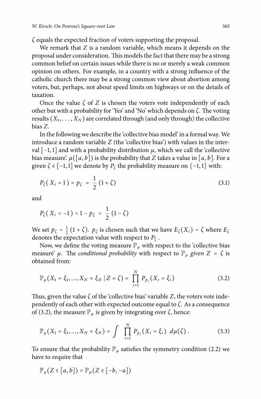
ζ equals the expected fraction of voters supporting the proposal.We remark that Z is a random variable, which means it depends on the

proposal under consideration.ismodels the fact that theremay be a strong

common belief on certain issues while there is no or merely a weak common

opinion on others. For example, in a country with a strong inuence of the

catholic church there may be a strong common view about abortion among

voters, but, perhaps, not about speed limits on highways or on the details of

taxation.

Once the value ζ of Z is chosen the voters vote independently of eachother but with a probability for ‘Yes’ and ‘No’ which depends on ζ .e votingresults (X1 , . . . , XN) are correlated through (and only through) the collectivebias Z.In the followingwe describe the ‘collective biasmodel’ in a formal way. We

introduce a random variable Z (the ‘collective bias’) with values in the inter-val [−1, 1] and with a probability distribution µ, which we call the ‘collectivebias measure’. µ([a, b]) is the probability that Z takes a value in [a, b]. For agiven ζ ∈ [−1, 1] we denote by Pζ the probability measure on −1, 1 with:

Pζ(X i = 1 ) = pζ = 1

2(1 + ζ) (3.1)

and

Pζ(X i = −1 ) = 1 − pζ = 1

2(1 − ζ)

We set pζ = 1

2(1 + ζ). pζ is chosen such that we have Eζ(X i) = ζ where Eζ

denotes the expectation value with respect to Pζ .

Now, we dene the voting measure Pµ with respect to the ‘collective bias

measure’ µ. e conditional probability with respect to Pµ given Z = ζ isobtained from:

Pµ(X1 = ξ1 , ..., XN = ξN ∣ Z = ζ) =N

∏i=1

Ppζ (X i = ξ i) (3.2)

us, given the value ζ of the ‘collective bias’ variable Z, the voters vote inde-pendently of each other with expected outcome equal to ζ . As a consequenceof (3.2), the measure Pµ is given by integrating over ζ , hence:

Pµ(X1 = ξ1 , ..., XN = ξN) = ∫N

∏i=1

Ppζ (X i = ξ i) dµ(ζ) . (3.3)

To ensure that the probability Pµ satises the symmetry condition (2.2) we

have to require that

Pµ(Z ∈ [a, b]) = Pµ(Z ∈ [−b,−a])


i.e.

µ([a, b]) = µ([−b,−a]) (3.4)

e probability measure Pµ denes a whole class of examples, each (sym-

metric) probability measure µ on [−1, 1] denes its unique Pµ . For example,

if we choose µ = δ0, i.e. µ([a, b]) = 1 if a ≤ 0 ≤ b and = 0 otherwise, we ob-tain independent random variables X i as discussed in the nal part of section

2. Indeed, µ = δ0 means that Z = 0, consequently (3.3) denes independentrandomvariables. Observe, that this is the onlymeasure forwhich Z assumesa xed value, since the collective bias measure µ has to be symmetric (3.4).Another interesting example is the case when µ is the uniform distribu-

tion on [−1, 1], meaning that each value in the interval [−1, 1] is equally likely.is case was considered by Stran (Stran 1982). He observed that this

model is intimately connected with the Shapley-Shubik power index. We

will comment on this interesting connection and on Stran’s calculation in

an appendix (section .1). To apply the ‘collective bias’ model to a given het-

erogeneous votingmodel we have to specify themeasure µ, of course. In fact,thismeasuremay change from state to state. In particular, onemay argue that

larger states tend to have a less homogeneous population and hence, for ex-

ample, the inuence of a specic religious or political group will be smaller.

As an example to this phenomenon, we will later discuss a model modify-

ing Stran’s example where µ(dz) = 1

2χ[−1,1](z) dz (uniform distribution in

[−1, 1]) to a measure where µN depends on the population N , namely

µN(dz) =1

2aNχ[−aN ,aN ](z)dz (3.5)

with parameters 0 < aN ≤ 1. In particular, if we have aN → 0 as N → ∞,the parameter aN reects the tendency of a common belief to decrease witha growing population.

Except for the trivial case µ = δ0 the random variables X i are never inde-

pendent under Pµ .is can be seen from the covariance

⟨X i , X j⟩µ ∶= Eµ(X iX j) −Eµ(X i)Eµ(X j) . (3.6)

In (3.6) as well as in the following Eµ denotes expectation with respect to

Pµ . In fact, the random variables X i are always positively correlated:

eorem 3.1 For i ≠ j we have

⟨X i , X j⟩µ = ∫ ζ2 dµ(ζ) . (3.7)


e quantity ∫ ζ2 dµ(ζ) is called the second moment of the measure µ.Since the rst moment ∫ ζ dµ(ζ) vanishes due to (3.4) the second momentequals the variance of µ. Observe that ∫ ζ2dµ(ζ) = 0 implies µ = δ0. Forindependent random variables ⟨X i , X j⟩µ = 0, so (3.7) implies that X i , X jdepend on each other unless µ = δ0.To investigate the impact of the collective bias measure µ on the ideal

weight in a heterogeneous voting model we have to compute the quantity

Eµ(∣N

∑i=1

X i ∣) (3.8)

for a measure µ and population N (at least for large N).is is done withthe help of the following theorem:

eorem 3.2 We have:

∣ Eµ(1

N∣N

∑i=1

X i ∣) − ∫ ∣ζ ∣ dµ(ζ)∣ ≤ 1√N

(3.9)

Let us dene µ = ∫ ∣ζ ∣ dµ(ζ). If we choose µ ≠ δ0 independent of the (popu-lation of the) stateeorem 3.2 implies that the optimal weight in the coun-

cil is proportional to N (rather than√N). is is true in particular for the

original Stran model (Stran 1982) where µn ≡ 1

2χ[−1,1](z) dz which cor-

responds to the Shapley-Shubik power index (see section .1). We have:

eorem 3.3 If the collective bias measure µ ≠ δ0 is independent of N thenthe optimal weight in the council is given by:

wN = Eµ(N

∑i=1

∣X i ∣) ∼ µ N (3.10)

If µ = µN depends on the population then

EµN (∣N

∑i=1

X i ∣) ∼ N µN

as long as µN ≥ 1

N 1/2−ε for some ε > 0. However, if µN ≤ 1

N 1/2+ε , then

EµN (∣N

∑i=1

X i ∣) ∼√N .

Hence, in this case we rediscover a square-root law.

We summarize:


eorem 3.4 Let us suppose that a state with a population of size N is char-acterized by a collective bias measure µN , then:

1. If

µN = ∫ ∣ζ ∣ dµN(ζ) ≥ C1

N 1/2−ε (3.11)

for some ε > 0 and for all large N then the optimal weight wN is given

by:

wN = Eµ( ∣N

∑i=1

X i ∣ ) ∼ N µN . (3.12)

2. If

µN = ∫ ∣ζ ∣ dµN(ζ) ≤ C1

N 1/2+ε (3.13)

then for large N the optimal weight wN is given by:

wN = Eµ( ∣N

∑i=1

X i ∣ ) ∼√N . (3.14)

Example In our Stran-type example (3.5) we choose:

µN(dz) =1

2aNχ[−aN ,aN ](z)dz, (3.15)

then:

µN = 12aN . (3.16)

Let us assume aN ∼ C N−α for 0 ≤ α ≤ 1. en, if α > 1

2we have wN ∼

√N

and if α < 1

2we obtain wN ∼ C N 1−α .

Remarks 3.5

1. Our result shows that in all cases the optimal weight wN satises

C√N ≤ wN ≤ N . It is a matter of empirical studies to determine

which measure µN is appropriate to the given voting system. Any of

the empirical results of (Gelman et al. 2004) can be modeled by an

appropriate choice of µN .

2. It is only µN that enters the formulae (3.12) and (3.14), no other infor-

mation about µN is relevant.e quantities µN can be estimated using

eorem 3.2. In fact, more is true by the following result.


eorem 3.6 Let PN be the distribution of 1N ∑Ni=1 X i under the measure

PµN then the sequence of measures PN − µN converges weakly to 0.

eorem 3.6 tells us that the collective biasmeasure can be recovered from

voting results. Let us denote by S a voting result, i. e. S = 1

N ∑Ni=1 X i . In other

words, 12(S + 1) is the fraction of armative votes.eorem 3.6 tells us that

the probability distribution of S approximates the measure µN for large N .On the other hand the distribution of S can be estimated from independentvoting samples (dening the empirical distribution).

Note that the empirical distribution of voting results 1

N ∑Ni=1 X i is the

quantity considered in (Gelman et al. 2004). eorem 3.6 tells us that the

distribution of the voting results for large number N of voters is approxi-mately equal to the distribution µN . In particular, in the case of independent

voters the voting result is always extremely tight while for Stran’s example

any voting result has the same probability, i.e. it is equally likely that a pro-

posal gets 99% or 53% of the votes.e general ‘collective biasmodel’ dened

above is an extension both of the independent voting model and of Stran’s

model.is general model can be t to any distribution of voting results.

4. Voting models as spin systems

Spin systems are a central topic in statistical physics. ey model magnetic

phenomena.e spin variables, usually denoted by σi , may take values in the

set −1,+1 with +1 and −1 meaning ‘spin up’ and ‘spin down’ respectively.e spin variables model the elementary magnets of a material (say the elec-

trons or nuclei in a solid).e index i runs over an index set I which repre-sents the set of elementarymagnets. Wemay (and will) take I = 1, 2, . . . ,Nin the following.

A spin conguration is a sequence σii∈1, . . . ,N ∈ −1,+1N . A congura-tion of spins σii∈I has a certain energywhich depends on the way the spinsinteractwith each other and (possibly) an exteriormagnetic eld.e energy,

a function of the spin conguration, is usually denoted by E = E(σii∈I).Spin systems prefer congurations with small energy. For example in so

called ferromagnetic systems,magneticmaterials we encounter in every day’s

life, the energy of spins pointing in the same direction is smaller than the one

for antiparallel spins, hence there is a tendency that spins line up, a fact that

leads to the existence of magnetic materials.

e temperature T measures the strength of uctuations in a spin system.If the temperature T of a system is zero, there are no uctuations and thespins will stay in the conguration(s) with the smallest energy. However, if

the temperature is positive, there is a certain probability that the spin con-

guration deviates from the one with the smallest energy.e probability to


nd a spin system at temperature T > 0 in a a conguration σi is given by:

p (σi) = Z−1 e −1T E(σ i) (4.1)

e quantity Z is merely a normalization constant, to ensure that the righthand side of (4.1) denes a probability (i. e. gives total probability equal to

one). Consequently:

Z = ∑σ i∈−1,1N

e −1T E(σ i) (4.2)

A probability distribution as in (4.1) is called aGibbs measure. It is customaryto introduce the inverse temperature β = 1

T and to write (4.1) as:

p (σi) = Z−1 e −β E(σ i) (4.3)

ere is a reason to introduce spin systems here: Obviously, any spin sys-

tem can be interpreted as a voting system, we just interchange the words spin

conguration and voting result as well as the symbols σi and X i . In fact, a

Gibbs measure p (as in (4.3)) denes a voting system with voting measure p,as long as E(σi) = E(−σi), so that p satises the symmetry condition(2.2). Moreover, any voting measure can be obtained from a Gibbs measure.

In particular, independent voting corresponds to the energy functional

E(σi) ≡ 1. In this case any conguration has the same energy, so that noconguration is more likely than any other.

e ‘collective bias’ model is given by an energy function:

E(σi) = − h ∑i

σi (4.4)

where h is a random variable connected to the collective bias variable Z by:

1

2(1 + Z) = eh

eh + e−h. (4.5)

Note, when h runs from −∞ to∞ in (4.5) the value of Z runs monotonouslyfrom −1 to +1.In term of statistical physics in this model the spins do not interact with

each other, but they do interact with a random but constant exterior eld.

e inverse temperature β is superuous in this model as it can be absorbedin the magnetic eld strength h.

5. e voters’ interaction model

In the collective bias model the voting behavior of each voter is inuenced by

a preassigned, a priori given collective bias variable Z (by an exterior mag-netic eld in the spin picture). e correlation between the voters results

from the general voting tendency described by the value of Z.


In this section we investigate a model with a direct interaction betweenthe voters, namely a tendency of the voters to vote in agreement with each

other. In the view of statistical physics this corresponds to the tendency of

magnets to align.ere are various models in statistical physics to prescribe

such a situation. Presumably the best known one is the Ising model where

neighboring spins interact in the prescribed ways.e neighborhood struc-

ture is most of the time given by a lattice (e.g. Zd ).e results on the system

depend strongly on that neighborhood structure, in the case of the lattice Zd

on the dimension d.In the following we consider another, in fact easier model where no such

assumption on the local ‘neighborhood’ structure has to be made. We con-

sider it an advantage of the model that very little of the microscopic correla-

tion structure of a specic voting system enters into the model.

e model we are going to consider is known in statistical mechanics as

the Curie-Weiss model or the mean eld model (see e.g. (ompson 1972),(Bolthausen and Sznitman 2002) or (Dorlas 1999)). In this model a given

voter (spin) interacts with all the other voters (resp. spins) in a way which

makes it more likely for the voters (spins) to agree than to disagree. is

is expressed through an energy function E which is smaller if voters agree.Note that a small energy for a given voting conguration (relative to the othercongurations) leads to a high probability of that conguration relative to theothers through formula (4.3).

e energy E for a given voting outcome X ii=1. . .N is given in the meaneld model by:

E(X i) = − JN − 1 ∑i , j

i/= j

X iX j . (5.1)

Here J is a non negative number called the coupling constant. According to(5.1) the energy contribution of a single voter X i is expressed through the

averaged voting result of all other voters 1

N−1 ∑ j/=i X j . If X i agrees in sign

with this average the voter imakes a negative contribution to the total energy,otherwise X i will increase the total energy. e strength of this negative or

positive contribution is governed by the coupling constant J. In other words:Situations for which voter i agrees with the other voters in average are morelikely than others.is can be seen from the formula for the probability of a

given voting outcome, namely:

p (X i) = Z−1 e− β E(X i) = Z−1 e β J 1N−1 ∑i/= j X iX j (5.2)

where as before

Z = ∑X i∈±1N

e− β E(X i) . (5.3)


Since the probability density p depends only on the product of β and J wemay absorb the parameter J into the inverse temperature β. So without lossof generality we can set J = 1. We denote the probability density (5.2) by pβ ,Nand the corresponding expectation by Eβ ,N .

Our goal is to compute the average:

wN = E β ,N( ∣N

∑i=1

X i ∣ ). (5.4)

e quantity wN gives the optimal weight in the council for a population

of N voters with a correlation structure given by a mean-eld model withinverse temperature β. We will see that the value ofwN changes dramatically

when β changes from a value below one to a value above one.is has to dowith the fact that the mean-eld model undergoes a phase transition at the

inverse temperature β = 1 (see (Bolthausen and Sznitman 2002; Dorlas 1999;ompson 1972)).

eorem 5.1

1. If β < 1 then

wN = Eβ ,N( ∣N

∑i=1

X i ∣ ) ∼√2√π

1√1 − β

√N as N →∞. (5.5)

2. If β > 1 then

wN = Eβ ,N( ∣N

∑i=1

X i ∣ ) ∼ C(β) N as N →∞. (5.6)

Remarks 5.2

1. By xN ∼ yN as N →∞ we mean that limn→∞xNyN

= 1.

2. e constant C(β) in (5.6) can be computed: If β > 1 then C(β) is the(unique) positive solution C of

tanh(β C) = C . (5.7)

Note that for β ≤ 1 there is no positive solution of equation (5.7).

eorem 5.1 can be understood quite easily on an intuitive level. We recall

that the temperature T measures the strength of uctuations, in other words:Low temperature (= large β = 1

T ) means high order in the system, high tem-

perature (= small β) means disorder. Hence, the theorem says, that for strong


order the expected voting result is well above (resp. well below) 50 % and the

ideal weight is proportional to the size of the population, while for highly

uctuating societies polls are as a rule very tight and one obtains a square

root law for the ideal representation.

e proof ofeorem 5.1 will be given in section .4.

6. Conclusions

e above calculations show that one can reproduce the square-root law as

well as the results of (Gelman et al. 2004) and other laws by assuming par-

ticular correlation structures among the voters of a certain country. To nd

the right model is a question of adjusting the parameters of the models to

empirical data of the country under consideration. Moreover, the models al-

low us to investigate questions about voting systems on a theoretical level.

We believe that the models described above can help to understand voting

behavior in many situations.

To design a nonhomogeneous voting system for a constitution in the lightof our results is a question of dierent nature. Even knowing the correlation

structure of the countries in question exactly would be of limited value to

design a constitution. Constitutions are meant for a long term period, cor-

relation structures of countries on the other hand are changing even on the

scale of a few years.

One might argue that modern societies have a tendency to decrease the

correlation between their members. In all modern states, at least in theWest,

the inuence of churches, parties, and unions is constantly declining.

In addition to this it seems more important to protect small countries

against a domination of the big ones than the other way round. is mo-

tivates us to choose a square-root law in these long term cases.

Appendix

A Power indices and Stran’s model

Here we investigate some connection of our models with power indices.

Power indices are usually dened through the ability of voters to change the

voting result by their vote. To dene power indices so we have to introduce a

general setup for voting systems.is extends the considerations of the rest

of this paper where we considered only weighted voting. Our presentation

below is inspired by (Laruelle and Valenciano 2005) and (Stran 1982).

Let V = 1, . . . ,N be the set of voters.e (microscopic) voting outcomeis a vector X = (X1 , . . . , XN) ∈ −1,+1N . Of course, X i = 1 means thatthe voter i approves the proposal under consideration, while X i = −1 meansi rejects the proposal. We call Ω = −1,+1N together with a probability


measure P a voting space, if P is invariant under the transformation T ∶ ω ↦−ω, thusP(X) = P(−X) (see section 2 for a discussion of this property).A voting rule is a function ϕ ∶ −1,+1N Ð→ −1,+1. e voting rule

associates to a microscopic voting outcome X = (X1 , . . . , XN) a macroscopicvoting result, i. e. the decision of the assembly.us, ϕ(X) = 1 (resp. ϕ(X) =−1) means that the proposal is approved (resp. rejected) by the assembly Vif the microscopic voting outcome is X = (X1 , . . . , XN). We always assumethat the voting rule ϕ ismonotone: If X i ≤ Yi for all i then ϕ(X) ≤ ϕ(Y). Wealso suppose that ϕ(−1, . . . ,−1) = −1 and ϕ(+1, . . . ,+1) = +1.Following (Laruelle and Valenciano 2005) we say that a voter i is suc-

cessful for a voting outcome X if ϕ(X) = X i . Let us set (X1 , . . . , XN)i ,− =(X1 , . . . , X i−1 ,−X i , X i+1 , . . . , XN). We call a voter i decisive for X if ϕ(X) ≠ϕ(X i ,−), i. e. if the voting result changes if i changes his/her mind.Given a voting space (−1, 1N ,P) and a voting rule ϕ we dene the (P-

)power index β by:

β(i) = βP (i) = PX ∈ −1,+1N ∣ i is decisive for X (A.1)

Laruelle and Valenciano (Laruelle and Valenciano 2005) show that many

known power indices are examples of the general concept (A.1). For exam-

ple it is not dicult to show that one obtains the total Banzhaf index (see

(Banzhaf 1965) or (Taylor 1995)) if P is the probability measure of indepen-dent voting.

If we take P = Pµ to be the voting measure corresponding to the col-

lective bias measure µ we get a whole family of power indices from (A.1).Stran (Stran 1982) (see also (Paterson Preprint)) demonstrates that if µ isthe uniform distribution on [−1, 1] then βPµ is just the Shapley-Shubik index

(see (Shapley and Shubik 1954) or (Taylor 1995)).

In a subsequent publication on general power indiceswewill give a deriva-

tion of this fact in the current framework.

B Proofs for section 2

We start with a short Lemma:

Lemma B.1 Suppose X1 , ..., XN are −1, 1−valued random variables withthe symmetry property (2.2) then

E(N

∑i=1

X i) = 0 (B.1)

and


E(N

∑i=1

X i χ(N

∑i=1

X i)) = E(∣N

∑i=1

X i ∣) . (B.2)

Remark B.2 As dened above χ(x) = 1 if x > 0, χ(x) = −1 if x ≤ 0.

Proof (2.2) implies

P(X i = 1) = P(X i = −1) =1

2

hence E(X i) = 0 and (B.1) follows.To prove (B.2) we observe that

E(∣N

∑1

X i ∣) = E(N

∑i=1

X i ;N

∑i=1

X i > 0) −E(N

∑i=1

X i ;N

∑i=1

X i < 0)

= E(N

∑i=1

X i χ(N

∑i=1

X i)) . ◻

We turn to the proof ofeorem 2.1.

Proof (eorem 2.1) Let us abbreviate: Sν ∶= ∑Nνi=1 Xν i .

Observe that the Sν are independent by assumption and satisfyE(Sν) = 0,moreover

E(Sν χ(Sµ)) = 0 if ν ≠ µ (B.3)

and

E(Sν χ(Sν)) = E(∣Sν ∣) (B.4)

by Lemma B.1. To nd the minimum of the function

∆(w1 , ...,wM) = E((M

∑1

Sν −M

∑1

wν χ(Sν))2)

we look at the zeros of ∂∆∂wµ.

0 = ∂∆∂wµ

= −2 E((M

∑1

Sν −M

∑1

wν χ(Sν))χ(Sµ))


= −2 E(Sµ χ(Sµ) −wµ χ(Sµ) χ(Sµ)) . (B.6)

So

wµ E((χ(Sµ))2) = E(Sµ χ(Sµ)) = E(∣Sµ ∣) .

Since χ(Sµ)2 = 1 we obtain

wµ = E(∣Sµ ∣) . ◻

We turn to the proof ofeorem 2.2.

Proof Let X1 , ..., XN be −1, 1−valued random variables withP(X i = 1) = P(X i = −1) = 1

2.en

E(∣N

∑1

X i ∣) =√N E(∣ 1√

N

N

∑1

X i ∣) .

By the central limit theorem (see e.g. (Lamperti 1996)) 1√

N ∑N1 X i has asymp-

totically a normal distribution with mean zero and variance 1, hence

E(∣ 1√N ∑

N1 X i ∣)→

√2

√π . ◻

C Proofs for section 3

Proof (eorem 3.1) Since Eµ(X i) = 0,

⟨X i , X j⟩µ = Eµ(X iX j)

= Pµ(X i = X j = 1) + Pµ(X i = X j = −1) − 2Pµ(X i = 1, X j = −1)

= ∫ dµ(ζ) P 12(1+ζ)(X i = X j = 1) + P 1

2(1+ζ)(X i = X j = −1)

−2P 12(1+ζ)(X i = 1, X j = −1)

= ∫ dµ(ζ) 14(1 + ζ)2 + 1

4(1 − ζ)2 − 1

2(1 − ζ2)

= ∫ ζ2dµ(ζ) . (C.1)

◻

To proveeorem 3.2 we need the following Lemma:

Lemma C.1 Eµ( 1N ∣∑(X i − Z)∣) ≤ 1√

N.


Proof

Eµ(1

N∣∑(X i − Z)∣) = 1

NEµ(∣∑(X i − Z)∣)

≤ 1N

Eµ((∑(X i − Z))2)1/2

= 1N

∫ dµ(ζ) Epζ((N

∑1

(X i − ζ))2)1/2

. (C.2)

Given Z = ζ the random variables X i−ζ havemean zero and are independentwith respect to the measure Ppζ , thus

Epζ((N

∑1

(X i − ζ))2) = NEpζ (X i − ζ)2 = N(1 − ζ2) ≤ N ,

hence

(C .2) ≤ 1√N

(∫ dµ(ζ)(1 − ζ2))1/2 ≤ 1√N. ◻

Using Lemma C.1 we are in a position to proveeorem 3.2:

Proof (1) Suppose that:

µN = ∫ ∣ζ ∣ dµN(ζ) ≥ C1

N 1/2−ε (C.3)

then we estimate:

EµN (1

N∣N

∑1

X i ∣) = EµN (∣1

N

N

∑1

(X i − Z) + Z∣) (C.4)

≤ EµN (∣Z∣) +EµN (∣1

N

N

∑1

(X i − Z)∣) ≤ µN +1√N

(C.5)

by Lemma C.1. Moreover

EµN (1

N∣N

∑1

X i ∣) ≥ EµN (∣Z∣) −EµN (∣1

N∑X i − Z∣) ≥ µN −

1√N.

Hence

∣EµN (1

N∣N

∑1

X i ∣) − µN ∣ ≤ 1√N

(C.7)


which proves (3.12).

(2) To prove (3.14) we obtain by the same reasoning as above:

∣EµN (1

N∣N

∑1

X i ∣) − µN ∣ ≤ 1√N

(C.8)

◻

We end this section with the proof ofeorem 3.6:

Proof We have to prove that for bounded continuous functions f :

∫ ( f ( 1N

N

∑i=1

X i) − f (Z) ) d PµN → 0. (C.9)

e convergence (C.9) is clear for continuously dierentiable f fromLemma C.1. It follows for arbitrary bounded continuous f by a densityargument. ◻

D Proofs for section 5

In this section we proveeorem 5.1.

Proof (eorem 5.1 (1)) We denote by E(N)

0 the expectation of the coin toss-

ing model for N independent symmetric +1,−1-valued random variables,i.e.:

E(N)

0(F(X1 , . . . , XN)) = 1

2N∑

x i∈+1,−1N

f (x1 , . . . , xN). (D.1)

We set:

ZβN = E(N)

0 ( eβ2( 1√

N ∑Ni=1 X i)

2

) (D.2)

and:

XβN = E(N)

0 ( ∣ 1√N

N

∑i=1

X i ∣ eβ2( 1√

N ∑Ni=1 X i)

2

). (D.3)

en:

EβN(∣N

∑i=1

X i ∣) =√NXβ ,N

Zβ ,N. (D.4)

Under the probability law E(N)

0 the random variables X i are centered and

independent, thus the central limit theorem (see e.g. (Lamperti 1996)) tells us


that 1√

N ∑Ni=1 X i converges in distribution to a standard normal distribution.

Consequently, for β < 1 and N →∞ :

ZβN →1√2π ∫

∞

−∞e −

(1−β) x2

2 dx = 1√1 − β

(D.5)

and:

XβN →1√2π ∫

∞

−∞∣x∣ e −

(1−β) x2

2 dx =√2√π

1

1 − β. (D.6)

Consequently:

EβN(∣N

∑i=1

X i ∣) =√NXβ ,N

Zβ ,N∼

√2√π

1√1 − β

√N . (D.7)

◻

Proof (eorem 5.1 (2)) Byeorem6.3 in (Bolthausen and Sznitman 2002)

the distribution νN of SN = 1

N ∑Ni=1 X i converges weakly to the measure ν =

δ−C(β) + δC(β) where C(β) was dened in (5.7).Hence,

Eβ(∣N

∑i=1

X i ∣) = N Eβ(∣SN ∣) = N ∫ ∣λ∣ dνN(λ)

≈ N ∫ ∣λ∣ dν(λ) = N C(β). (D.8)

◻

Acknowledgements

It is a pleasure to thank Hans-Jürgen Sommers, Duisburg-Essen, and Woj-

ciech Słomczyński and Karol Życzkowski, Krakow, for valuable discussions.

e author would also like to thank Helmut Hölzler, Göttingen, for pointing

out a notational inconsistency in a previous version of the paper.

References

Banzhaf, J. (1965). Weighted Voting Doesn’t Work: AMathematical Analysis. RutgersLaw Review 19: 317–343.

Bolthausen, E. and Sznitman, A. (2002). Ten lectures on random media.Dorlas, T. (1999). Statistical Mechanics. Institute of Physics Publishing.


Felsenthal, D. and Machover, M. (1998).e measurement of power: theory and prac-tice, problems and paradoxes. Edward Elgar.

Gelman, A., Katz, J. and Bafumi, J. (2004). Standard voting power indexes don’t work:

an empirical analysis. British Journal of Political Science 34: 657–674.Kirsch, W. (Preprint). On the distribution of power in the Council of ministers of the

EU. Available from http://www.ruhr-uni-bochum.de/mathphys/.

Lamperti, J. (1996). Probability. Wiley.Laruelle, A. and Valenciano, F. (2005). Assessing success and decisiveness in voting

situations. Social Choice and Welfare 24: 171–197.Paterson, I. (Preprint). A Lesser Known Probabilistic Approach to the Schapley-

Shubik Index and Useful Related Voting Measures.

Shapley, L. and Shubik, M. (1954). A method for evaluating the distribution of power

in a commitee system. American Political Science Review 48: 787–792.Stran, P. (1982). Power indices in politics. In Brams, S. J., Lucas, W. F. and Stran,

P. D. (eds), Political and related models. Springer.Taylor, A. (1995).Mathematics and Politics. Springer.ompson, C. (1972).Mathematical Statistical Mechanics. Princeton University Press.

Documents

On Penrose's Square-root Law and Beyond - Homo Oeconomicus