On Some Optimal Control Problems for Electric Circuits

Kristof Altmann, Simon Stingelin, and Fredi Troltzsch

October 12, 2010

Abstract

Some optimal control problems for linear and nonlinear ordinary differential equations related to the optimalswitching between different magnetic fields are considered. The main aim is to move an electrical initial currentby a controllable voltage in shortest time to a desired terminal current and to hold it afterwards. Necessaryoptimality conditions are derived by Pontryagin’s principle and a Lagrange technique. In the case of a linearsystem, the principal structure of time-optimal controls is discussed. The associated optimality systems aresolved by a one-shot strategy using a multigrid software package. Various numerical examples are discussed.

1 Introduction

We consider a class of optimal control problems governed by linear and nonlinear systems of ordinary differentialequations (ODEs) with some relation to eddy current problems in continuum mechanics. The background of ourresearch in real applications is the magnetization of certain 3D objects. More precisely, it is the optimal switchingbetween different magnetization fields that stands behind our investigations.

Problems of this type occur in measurement sensors. If the measurement signal is much smaller than the noise,one uses differential measurement techniques, where one has to switch from one state to an other. In this paper, thesignal source would be an electromagnetic field. In practice, the magnetization process is performed by the controlof certain induction coils, and the associated model is described by the Maxwell equations. The numerical solutionof these partial differential equations is demanding and the treatment of associated optimal control problems is quitechallenging. To get a first impression of the optimal control functions to be expected in such processes, we studyhere simplified models for electrical circuits based on ordinary differential equations. They resemble the behaviorthat is to be expected also from 3D models with Maxwell’s equations.

We shall study different types of electrical circuits and associated optimal control problems. In all problems,we admit box constraints to bound the control functions. Moreover, we also consider an electrical circuit with anonlinear induction function.

Mathematically, our main goal is twofold. From an application point of view, we are interested in the formof optimal controls for different types of electrical circuits. We discuss several linear and nonlinear models withincreasing level of difficulty. On the other hand, we present an optimization method that is, to our best knowledge,not yet common in the whole optimal control community. By a commercial code, we directly solve nonsmoothoptimality systems consisting of the state equation, the adjoint equation and a projection formula for the control.This method was already used by several authors. In particular, it was suggested by Neitzel et al. [10] for optimalcontrol problems governed by partial differential equations. This approach works very reliably also for our problems.

We derive the optimality systems in two different ways. First, we invoke Pontryagin’s principle to obtain thenecessary information. While this approach is certainly leading to the most detailed information on the optimalsolutions, is may be difficult to apply in some cases. Therefore, we later establish the optimality conditions also bythe well known Lagrange principle of nonlinear optimization in function spaces, see e.g. Ioffe and Tikhomirov [6].This approach is easier to apply and turns out to be completely sufficient for numerical purposes.

The structure of the paper is as follows: Each model is discussed in a separate section. Here, we motivate theused ordinary differential equation, then we define the related optimal control problem and show its well-posedness.Next, we derive necessary optimality conditions. Finally, we suggest a numerical method and show its efficiency bynumerical tests.

1

Rc

Lu

i

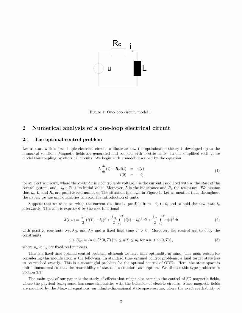
Figure 1: One-loop circuit, model 1

2 Numerical analysis of a one-loop electrical circuit

2.1 The optimal control problem

Let us start with a first simple electrical circuit to illustrate how the optimization theory is developed up to thenumerical solution. Magnetic fields are generated and coupled with electric fields. In our simplified setting, wemodel this coupling by electrical circuits. We begin with a model described by the equation

Ldi

dt(t) +Rc i(t) = u(t)

i(0) = −i0(1)

for an electric circuit, where the control u is a controllable voltage, i is the current associated with u, the state of thecontrol system, and −i0 ∈ R is its initial value. Moreover, L is the inductance and Rc the resistance. We assumethat i0, L, and Rc are positive real numbers. The situation is shown in Figure 1. Let us mention that, throughoutthe paper, we use unit quantities to avoid the introduction of units.

Suppose that we want to switch the current i as fast as possible from −i0 to i0 and to hold the new state i0afterwards. This aim is expressed by the cost functional

J(i, u) =λT

2(i(T )− i0)2 +

λQ

2

∫ T

0

(i(t)− i0)2 dt+λU

2

∫ T

0

u(t)2 dt (2)

with positive constants λT , λQ, and λU and a fixed final time T > 0. Moreover, the control has to obey theconstraints

u ∈ Uad = u ∈ L2(0, T ) |ua ≤ u(t) ≤ ub for a.a. t ∈ (0, T ), (3)

where ua < ub are fixed real numbers.

This is a fixed-time optimal control problem, although we have time optimality in mind. The main reason forconsidering this modification is the following: In standard time optimal control problems, a final target state hasto be reached exactly. This is a meaningful problem for the optimal control of ODEs. Here, the state space isfinite-dimensional so that the reachability of states is a standard assumption. We discuss this type problems inSection 3.3.

The main goal of our paper is the study of effects that might also occur in the control of 3D magnetic fields,where the physical background has some similarities with the behavior of electric circuits. Since magnetic fieldsare modeled by the Maxwell equations, an infinite-dimensional state space occurs, where the exact reachability of

2

states is a fairly strong assumption. Therefore, we prefer to approximate the target state closely in a short timerather than to reach it. This is expressed in the setting above.

We search for a couple (i∗, u∗), which minimizes this functional subject to the initial-value problem (1), and theconstraints (3). The state function i is considered as a function of H1(0, T ). The functions i∗ and u∗ are calledoptimal state and optimal control, respectively.

The cost functional will be minimal, if the current i∗(T ) is close to i0 (first term in J) and reaches this goal quitefast (second term), while the cost of u is considered by the third term. The weights λT , λQ, and λU can be freelychosen to balance the importance of these 3 terms. We should underline that we need a positive regularizationparameter λU for the theory and our numerical approach. First of all, this parameter is needed to set up ouroptimality systems in the form we need for our numerical method. For instance, we solve the optimality systems(15) or (16), where λU must not vanish. To have a convex functional, λU > 0 is needed. Moreover, it is knownthat other numerical optimization methods (say gradient methods, e.g.) behave less stable without regularisationparameter.

Since the state equation is linear, the objective functional is strictly convex, and the set of admissible controlsis nonempty and bounded in L2(0, T ), the existence of a unique optimal control is a standard conclusion. We shallindicate optimality by a star, i.e., the optimal control is u∗, while the associated optimal state is denoted by i∗.

2.2 The Pontryagin maximum principle

Let us derive the associated first-order necessary optimality conditions. There are at least two approaches. The firstis based on the theory of nonlinear programming in function spaces and uses the well-known concept of Lagrangemultipliers associated with the different types of constraints. To apply this technique, a Lagrange function has tobe set up and then the necessary conditions are deduced.

On the other hand, the celebrated Pontryagin maximum principle is a standard approach to tackle this problem.It contains the most complete information on the necessary optimality conditions. Therefore, we will apply thisprinciple and transform the associated results in a way that is compatible with the first approach. This is neededto interprete the adjoint state as the Lagrange multiplier associated with the state equation (1). In later sections,we prefer to apply the Lagrange principle.

Let us first recall the Pontryagin principle, formulated for the following class of optimal control problems withobjective functional of Bolza type:

min J(u) := g(x(T )) +∫ T

0f0(x, u) dt.

subject to

xk = fk(x, u) for k = 1, . . . , n,x(0) = x0,

u(t) ∈ Ω for a.a. t ∈ (0, T ),

(4)

where fk : Rn×Rm → R, k = 0, . . . , n, and g : Rn → R are sufficiently smooth functions, 0 is the fixed initial time,x0 is a fixed initial vector and Ω ⊂ Rm is a nonempty convex set of admissible control vectors; T > 0 is a fixed finaltime.

Associated with this problem, we introduce the dynamical cost variable x0 by

x0(t) = f0(x(t), u(t)), x0(0) = 0,

and the Hamilton function H : Rn+1 × Rn × Rm → R by

H(ψ, x, u) :=n∑

k=0

ψk fk(x, u). (5)

For n = 2, this readsH(ψ, x, u) := ψ0 f0(x, u) + ψ1 f1(x, u) + ψ2 f2(x, u). (6)

By the Hamilton function, the adjoint equation associated with a pair (x(·), u(·)) is defined by

ψi = −∂H∂xi

for i = 0, . . . , n, (7)

3

or, written in more explicit terms,

ψi(t) = −n∑

k=0

∂fk

∂xi(x(t), u(t))ψk(t) for i = 0, . . . , n. (8)

This is a linear system of differential equation for the vector function ψ. Notice that (8) implies ψ0 = 0 because fdoes not depend on x0, hence ψ0 is identically constant. Each solution ψ : [0, T ] → Rn+1, ψ(·) = (ψ0(·), . . . , ψn(·))>,of this adjoint equation is called adjoint state associated with the pair (x(·), u(·)).

Now we have all pre-requisites to formulate the Pontryagin maximum principle. Basic references for this opti-mality condition are Boltjanski et al. [12] or Ioffe / Tikhomirov [6], at least for a variable final time and a costfunctional containing only the integral part of J . Functionals of Bolza type with fixed final time T , as the problem isposed here, require some standard transformations to obtain the associated Pontryagin principle in its most commonform. We refer to the detailed discussion in Athans and Falb [2] or to the formulation in Pinch [11] or Feichtinger[3]. A review on different versions of the Pontryagin principle was given by Hartl et al. [5]. For problems withfunctional of Bolza type, unrestricted final state and fixed final time, which are autonomous in time, the followingversion holds true:

Theorem 1 (Pontryagin Maximum Principle). Let u∗(·) be an admissible control for the optimal control problem(4) with corresponding state x∗ = (x∗1, . . . , x

∗n). Then, in order that u∗ and x∗ minimize J subject to the given con-

straints, the following conditions must be satisfied: There exists a non-trivial adjoint state ψ(·) = (ψ0, ψ1, . . . , ψn)T :[0, T ] → Rn+1 that satisfies a.e. on (0, T ) the adjoint equation (8) with x(t) := x∗(t) and u(t) := u∗(t) togetherwith the terminal condition

ψi(T ) = ψ0∂g

∂xi(x∗(T )), i = 1, . . . , n,

and the Hamilton function H attains almost everywhere in (0, T ) its maximum with respect to u at u = u∗(t), i.e.

maxv∈Ω

H(ψ(t), x(t), v) = H(ψ(t), x∗(t), u∗(t)) for a.a. t ∈ (0, T ). (9)

Moreover, ψ0 is a nonpositive constant.

The adjoint equation (8) is a linear system for ψ(·). Therefore, the adjoint state ψ(·) cannot vanish at any timeunless it is identically zero. The latter case is excluded by the maximum principle. Therefore, it must hold ψ0 6= 0,since otherwise the terminal condition of the maximum would imply ψ(T ) = 0 and hence ψ(·) = 0. Re-defining ψby ψ := ψ/ψ0 and dividing (9) by |ψ0| we can therefore assume w.l.o.g that ψ0 = −1. This is a standard conclusionfor the type of problems above.

2.3 Necessary optimality conditions for the optimal control problem

In this part, we apply the Pontryagin maximum principle to derive the first order necessary optimality conditionsfor the optimal control u of the control problem (1) – (3).

Let us first explain how (1) – (3) fits in the problem (4), to which the Pontryagin principle refers. In (4), wemust define n, g, f0, . . . , fn, x, x0, and Ω. In (1) – (3), we have n = 1 and we define x1 := i, x0 := −i0. Moreover,f0, f1, and g are defined below. The set Ω is the interval [ua, ub]. In this way, (1) – (3) is related to (4), and wecan apply the Pontryagin principle to it. As a result, we will obtain the system (10), (11). Although (11) containsthe necessary information on an optimal control, it does not have the form we need for our numerical method.Therefore, in a second step, we transform (10), (11) to arrive at (15). This is the form we use for our numericalmethod. We recall that the control is pointwise bounded by real constants ua ≤ ub, i.e. u ∈ Uad. To cover theunbounded case, also ua = −∞ and/or ub = +∞ is formally allowed.

We re-write the differential equation (1) as

di

dt(t) = −Rc

Li(t) +

1Lu(t)

and definef1(i, u) := −Rc

Li+

1Lu.

4

The Bolza type objective functional in (4) is defined by

f0(i, u) :=λQ

2(i− i0)2 +

λU

2u2,

g(i) :=λT

2(i− i0)2.

As we explained at the end of the last section, we are justified to assume ψ0 = −1. Writing for convenienceψ := ψ1, we obtain

H = −(λQ

2(i− i0

)2 +λU

2u2

)+ ψ (−Rc

Li+

u

L).

From this definition of H, we obtain the adjoint equation

dψ

d t(t) = −∂ H

∂ i(t) = λQ

(i(t)− i0

)+ ψ(t)

Rc

L.

Furthermore, the Pontryagin principle yields the final condition

ψ(T ) = −∂ g∂ i

(i(T )) = −λT

(i(T )− i0

).

We have derived the following adjoint system:

dψ

dt(t) = −ψ(t)

Rc

L+ λQ

(i(t)− i0

)ψ(T ) = −λT (i(T )− i0).

(10)

As before, we denote the optimal quantities by i∗ and u∗ and omit the star at the associated adjoint state ψ.The constraint (3) is considered by the following variational inequality that is easily derived from the maximumcondition (9),

∂ H

∂ u(i∗(t), u∗(t), ψ(t))(u− u∗(t)) = (−λuu

∗(t) + ψ(t)/L)(u− u∗(t)) ≤ 0 ∀u ∈ Uad, for a.a. t ∈ (0, T ).

We write this in the more common form of a variational inequality,

−∂ H∂ u

(i∗(t), u∗(t), ψ(t))(u− u∗(t)) = (λuu∗(t)− ψ(t)/L)(u− u(t)∗) ≥ 0 ∀u ∈ Uad. (11)

In some sense, this form does not really fit to numerical computations. In order to arrive at the standard form ofnonlinear programming with associated Lagrange multipliers, we perform a substitution and transform the adjointstate ψ to a Lagrange multiplier p. To this aim, we set

p(t) = −ψ(t)L

, (12)

which impliesdp

dt(t) = − 1

L

dψ

d t(t).

We replace ψ by p in equations (10) and obtain the system

−Ldpdt

(t) = −Rc p(t) + λQ

(i(t)− i0

)−Lp(T ) = −λT (i(T )− i0).

(13)

Using the same substitution in equation (11), we find

(λUu∗(t) + p(t))(u− u∗(t)) ≥ 0 ∀u ∈ [ua, ub] and a.a. t ∈ (0, T ). (14)

5

Therefore, we can completely describe the optimal control u∗ by the following case study:

(i) λUu∗(t) + p(t) > 0 ⇒ u∗(t) = ua

(ii) λUu∗(t) + p(t) < 0 ⇒ u∗(t) = ub

(iii) λUu∗(t) + p(t) = 0 ⇒ u∗(t) = − 1

λUp(t).

A further discussion of these relations yields that the optimal control satisfies almost everywhere the well knownprojection formula

u∗(t) = P[ua,ub]−1λU

p(t) = max(min(ub,−1λU

p(t)), ua),

where P[α,β] denotes the projection of a real number on the interval [α, β]. For the derivation of this formula,we refer the reader e.g. to [14]. After inserting this expression for u∗ in (1) while considering also (13), the twounknowns i∗ and p satisfy the forward-backward optimality system

Ld i

d t(t) +Rc i(t) = P[ua,ub]−

1λU

p(t)i(0) = −i0

−L d pd t

(t) +Rc p(t) = λQ(i(t)− i0)

Lp(T ) = λT (i(T )− i0).

(15)

Although this is a nonlinear and nondifferentiable system, it can be easily solved numerically by available commercialcodes. In our computations, we applied the code COMSOL Multiphysics R©[1]. In the next section, we demonstratethe efficiency of this idea by numerical examples. There are various other numerical methods for solving systemsof ordinary differential equations. We only refer to the standard reference Hairer et al. [4]. Moreover, we mentionmethods tailored to the numerical treatment of electric circuits, which are presented in RosÃloniec [13]. We preferCOMSOL Multiphysics R©, because we were able to implement the solution of our nonsmooth optimality systemsin an easy way.

For convenience, we also mention the unbounded case ua = −∞ and ub = ∞. Here, we have

P[ua,ub]−1λU

p(t) = − 1λU

p(t),

hence the associated optimality system is in the unbounded case

Ld i

d t(t) +Rc i(t) = − 1

λUp(t)

i(0) = −i0−Ldp

dt(t) +Rc p(t) = λQ(i(t)− i0)

Lp (T ) = λT (i(T )− i0).

(16)

The unique solution to this system is the pair (i∗, p), and the optimal control is given by u∗ = −λ−1U p.

2.4 Numerical examples

In the examples, we select the bounds ua := −300 and ub := 300. Moreover, we consider the time interval [0, 1] andfix the constants i0 := 1, L := 3.5 and Rc := 145.

First, we investigate the influence of the parameters λT , λQ and λU . As explained above, we solve the nonlinearsystem (15) numerically to find the optimal solution. Let us start with the influence of λQ. This parameter controlsthe current i along the time. We fix λT and λU by 1 and vary λQ. Figure 2 shows how the current i approaches i0for increasing λQ. The larger λQ is, the faster the current approaches the target. The end of the curves is dependingon the ratio between λQ and λT . We discuss this below.

Next, we consider the influence of the control parameter λU . The other parameters are fixed by 1. Thisparameter expresses the cost of the control u. If λU is large, the control is expensive and it is more important tominimize |u|, cf. Figure 3. In its right hand side figure, we see that the upper bound ub is active at the beginning.

6

0.2 0.4 0.6 0.8 1.0

1.0

0.5

0.5

1.0i [A]

t [s]

λQ = 10

λQ = 1600

λQ = 6 · 105

λQ = 2.5 · 107

-

-

Figure 2: Electric current i by different λQ

0.2 0.4 0.6 0.8 1.0

1.0

0.5

0.5

1.0

i [A]

t [s]

λU = 10−3

λU = 10−5

λU = 10−6

λU = 10−7

−

−(a) Electric current i depending on λU

0.0 0.2 0.4 0.6 0.8 1.0

50

100

150

200

250

300u [V]

t [s]

λU = 10−3

λU = 10−5

λU = 10−6

λU = 10−7

(b) Voltage u depending on λU

Figure 3: Current i by different λU

Finally, we analyse all parameters more detailed and plot only the integral part

JQ :=∫ T

0

(i(t)− i0

)2dt

of the cost functional depending on the parameters. We are most interested in this part, since it expresses the speedof approaching i0. Our aim is to select parameters λQ and λU , where JQ is as small as possible. We fix λT = 1again. We vary only one of the parameters λQ and λU and set the other one to 1. Figure 4 shows the value ofJQ depending on λQ, respectively λU . The x-axis are scaled logarithmically. Both curves contain critical pointsbeyond which JQ grows considerably. In view of this, we recommend the choice λQ > 105 and λU < 10−4.

With nearly this ratio between λQ and λU , we try to find out a suitable λT . Fixing λQ = 106 and λU = 10−6,we vary λT . The left hand side of Figure 5 shows that the influence of λT on i is marginal almost everywhere.However, a zoom of the graph close to the final time T reveals that this parameter influences the final behavior. IfλT is large enough, i∗ ends near by i0.

We started with a simple circuit. In the next sections, we discuss some more examples of higher complexity.

2.5 A two-loop circuit modeled by a single ODE

In the remainder of this paper, we will consider several cases of electrical circuits with two loops. We start witha simple one and show that it can be still modeled by a single ODE. Therefore, this circuit still fits to the theoryof this section. This subsection is only to show how we transform this case to the single circuit case. Later, weconsider linear and nonlinear systems of two ODEs.

7

1000 105 107 109

0.2

0.4

0.6

0.8

1.0

JQ

λQ

(a) The value of Jq influenced by λQ

10 -4 0.01 1

0.2

0.4

0.6

0.8

1.0

10 -6

JQ

λU

(b) The value of Jq influenced by λU

Figure 4: Value JQ by different parameters

0.2 0.4 0.6 0.8 1.0

1.0

0.5

0.5

1.0

i [A]

t [s]

λT = 10

λT = 50

λT = 500

λT = 105

−

−(a) Electric current i depending on λT )

0.9975 0.9980 0.9985 0.9990 0.9995 1.00000.994

0.995

0.996

0.997

0.998

0.999

1.000i [A]

t [s]

λT = 105

λT = 500

λT = 50

λT = 10

(b) Electric current i depending on λT near T

Figure 5: Electric current depending on λT

Rc

Lu

Rw

i1 i2

i3A

B

I II

Figure 6: Electrical circuit with two loops

Consider the circuit of Figure 6 that contains an additional resistance Rw. Let us set up the differential equationsfor this circuit. Applying the Kirchhoff current law to node A, we get the equation

i1(t) = i2(t) + i3(t) (17)

at any time t. The electrical circuit is composed of the loops I and II. By the Kirchhoff voltage law, we obtain the

8

equations

Ldi3dt

(t) +Rc i1(t) = u(t) (18)

for loop I and

− Ldi3dt

(t) +Rw i2(t) = 0 (19)

for loop II. Our main interest is to control the current i3, which in the sequel is re-named by i := i3. From (17),(18) and (19), we deduce the following equation for the current i = i3:

L(1 +Rc

Rw)di

dt(t) +Rc i(t) = u(t).

With the initial condition i(0) = −i0, we arrive at the initial value problem

adi

dt(t) +Rc i(t) = u(t)

i(0) = −i0,(20)

where a is defined by

a := L (1 +Rc

Rw).

Our goal is to control the electrical currents such that the objective functional (2) is minimized. By our transfor-mation above, this modified problem, which consists of the new state equation (20), original cost functional (2) andcontrol constraints (3), is a particular case of the problem (1) – (3). Therefore, we obtain an optimality system thatis equivalent to (15) in the case of a bounded control and (16) for unbounded control. Because of this similarity,we abdicate of numerical examples.

3 Two loops coupled by inductances

3.1 The optimal control problem

In this section, we consider the optimal control of electrical circuits, which cannot be transformed easily to a singleODE. In the preceding sections, we derived the optimality system from the Pontryagin maximum principle andtransformed this result into the Lagrangian form. Here, we directly apply the Karush-Kuhn-Tucker theory (KKTtheory) of nonlinear programming problems in Banach spaces to deduce the optimality system. We do this in aformal way that does not explicitely mention the function spaces underlying the theory. The precise applicationof the standard Karush-Kuhn-Tucker theory to problems with differential equations is fairly involved, we refer,e.g., to Ioffe and Tikhomirov [6], Luenberger [8], or Jahn [7]. The assumptions of the KKT theory are met byall of our problems so that the same results will be obtained as the ones we derive below by the formal Lagrangetechnique, which is adopted from the textbook [14]. The optimality conditions obtained in this way are closer tothe applications of nonlinear programming techniques.

We consider the electrical circuit shown in Figure 7 with two loops coupled by inductances L1 and L2 via acoupling variable γ. In some sense, this model simulates the coupling between a magnetic field and eddy currents.For physical reasons, we require γ ∈ [0, 1].

This electrical circuit is modeled by the initial-value problem

L1di1dt

(t) + Cdi2dt

(t) +Rc i1(t) = u(t)

Cdi1dt

(t) + L2di2dt

(t) +Rwi2(t) = 0

i1(0) = −i0i2(0) = 0,

(21)

9

Rc

L1u

i1

L2 Rw

i2

I II

Figure 7: Model 2

which contains the ODEs for loop I and loop II, respectively. The constant C is defined by C := γ√L1L2. Now,

the cost functional to be minimized is defined by

J(i1, i2, u) :=λT

2(i1(T )− i0)2 +

12

∫ T

0

(λQ (i1(t)− i0)2 + λI i2(t)2 + λU u(t)2

)dt (22)

with nonnegative constants λT , λQ, λI and λU > 0.

The optimal control problem we consider in this subsection is to minimize (22) subject to the state equation(21) and to the box constraint (3).

To derive the associated optimality system, we might multiply the system of ODEs in (21) by the matrix Estanding in front of the derivatives dij/dt, j = 1, 2,

E =[L1 CC L2

](23)

to obtain a system of ODEs in standard form. This is, however, not needed here. We will use this approach forthe discussion of controllability in the next section. In contrast to the Pontryagin maximum principle, the formalLagrange principle is directly applicable to the system (21). Following the Lagrange principle, we ”eliminate” theODEs above by two Lagrange multiplier functions p1 and p2, respectively, while we keep the initial conditions andthe box constraint u ∈ Uad as explicit constraints. Therefore, the associated Lagrange function is defined by

L(i1, i2, u, p1, p2) := J(i1, i2, u)−∫ T

0

(L1di1dt

(t) + Cdi2dt

(t) +Rc i1(t)− u(t))p1(t) dt

−∫ T

0

(L2di2dt

(t) + Cdi1dt

(t) +Rw i2(t))p2(t) dt.

According to the Lagrange principle, the optimal solution (i∗1, i∗2, u

∗) has to satisfy the necessary optimality condi-tions of the problem to minimize L with respect to i1, i2, u without the ODE constraints but subject to the initialconditions and the box constraints. Notice that i1, i2, u are here decoupled. For i1, i2, this means

∂L∂ij

(i∗1, i∗2, u

∗, p1, p2)h = 0 ∀h with h(0) = 0, j = 1, 2.

With respect to u, the variational inequality

∂L∂u

(i∗1, i∗2, u

∗, p1, p2) (u− u∗) ≥ 0 ∀u ∈ Uad

must be satisfied. Let us write for short L = L(i∗1, i∗2, u

∗, p1, p2). For ∂L/∂u, we obtain

∂L∂u

(i∗1, i∗2, u

∗, p1, p2)u =∫ T

0

(λU u(t) + p1(t)) u(t) dt,

10

hence we have the variational inequality∫ T

0

(λU u∗(t) + p1(t)) (u(t)− u∗(t)) dt ≥ 0 ∀u ∈ Uad.

Again, the pointwise evaluation of the inequality leads finally to the projection formula

u∗(t) = P[ua,ub]−1λU

p1(t). (24)

For ∂ L/∂ i1, we deduce after integrating by parts

∂L∂i1

(i1, i2, u, p1, p2)h = λT (i1(T )− i0)h(T ) + λQ

∫ T

0

(i1(t)− i0)h(t) dt

−∫ T

0

(L1dh

dt(t) +Rc h(t)) p1(t) dt−

∫ T

0

Cdh

dt(t) p2(t) dt,

= λT (i1(T )− i0)− L1 p1(T )− C p2(T ) h(T )

+∫ T

0

λQ (i1(t)− i0)−Rc p1(t) + L1

dp1

dt(t) + C

dp2

dt(t)

h(t) dt

= 0 ∀h with h(0) = 0.

Since h(T ) and h(·) can vary arbitrarily, both terms in braces must vanish; hence the equations

−L1dp1

dt(t)− C

dp2

dt(t) +Rcp1(t) = λQ(i1(t)− i0(t))

L1 p1(T ) + C p2(T ) = λT (i1(T )− i0)(25)

must hold. In the same way, we derive from ∂ L/∂ i2 = 0 the equations

−C dp1

dt(t)− L2

dp2

dt(t) +Rwp2(t) = 0

C p1(T ) + L2 p2(T ) = 0.(26)

The equations (25) and (26) form the adjoint system. Collecting the equations (21), (24), (25), and (26), we obtainthe following optimality system to be satisfied by the optimal triple (i∗1, i

∗2, u

∗) and the associated pair of Lagrangemultipliers p1, p2:

L1di1dt

(t) + Cdi2dt

(t) +Rc i1(t) = P[ua,ub]−λ−1U p1(t)

Cdi1dt

(t) + L2di2dt

(t) +Rw i2(t) = 0

−L1dp1

dt(t)− C

dp2

dt(t) +Rc p1(t) = λQ (i1(t)− i0(t))

−C dp1

dt(t)− C L2

dp2

dt(t) +Rwp2(t) = λI i2(t)

i1(0) = −i0i2(0) = 0

L1 p1(T ) + C p2(T ) = λT (i1(T )− i0)

C p1(T ) + L2 p2(T ) = 0.

(27)

If the box constraints missing on u, then we can replace the nonlinear and nonsmooth term P[ua,ub]−λ−1U p1(t)

by the linear and smooth expression −λ−1U p1(t). To handle the numerical examples below, we directly solved the

nonsmooth optimality system (27) by the package COMSOL Multiphysics R©.

11

3.2 Numerical examples

In the problem above, we fix the final time T = 1 and the constants i0 := 1, L := 3.5, L2 := 2, Rc := 145, Rw :=3500 and γ = 0.9. Moreover, we impose the bounds ua := −300 and ub := 300 on the control.

First, we discuss a reasonable choice of the parameters λQ, and λU . Therefore, we define again

JQ :=∫ T

0

(i1(t)− i0

)2dt (28)

plot JQ for different parameters. As in Subsection 2.4, we select parameters, where JQ is as small as possible. Theparameters λT and λI have a very low influence on the size of JQ and we fix λT = 10000 and λI = 100. We varyonly one of the parameters λQ and λU and set the other one to 1. The left hand side of Figure 8 shows the valueof JQ depending on λQ and the right hand side depending on λU . We have nearly the same critical points as inmodel 1 (cf. Figure 4).

1 100 104 106 108

0.2

0.4

0.6

0.8

1.0

JQ

λQ

(a) Value of Jq depending on λQ (λU=1)

10 6 10 4 0.01 1

0.2

0.4

0.6

0.8

1.0

JQ

λU

(b) Value of Jq depending on λU (λQ=1)

Figure 8: Value of JQ by different parameters

Let us now plot the current i and the control u with the parameters λQ = 106, λU = 10−6, λT = 10000 andλI = 100 which have been found above. On the left hand side of Figure 9, we see how the current i approachesi0 = 1. Near the time t = 0 the control u stays at the upper bound ub, before it approaches the lower holding level(right hand side of Figure 9).

0.2 0.4 0.6 0.8 1.0

-1.0

-0.5

0.5

1.0

i [A]

t [s]

(a) Electric current i1

0.0 0.2 0.4 0.6 0.80

50

100

150

200

250

300

u [V]

t [s]

(b) Voltage u

Figure 9: Solution of Model 2

Additionally, we concentrate on the current i2. Because i2 is coupled with i1, we can neglect the time where i1is almost constant. Therefore, Figure 10 shows only a part of the time interval.

3.3 Time-optimal control

In the previous sections, we considered optimal control problems in a fixed interval of time. We formulated integralterms in the cost functional to reach the target state in short time. As we have explained in Section 2.1, we need

12

0.01 0.02 0.03 0.04

-0.08

-0.06

-0.04

-0.02

i [A]

t [s]

Figure 10: Current i2 in Model 2

this alternative, because this problem is only a first step for solving time-optimal control problems in the optimalswitching between magnetic fields. Then, the 3D Maxwell equations occur and it is really difficult to formulate atime-optimal problem in the right way.

However, in the case of ODEs, it is also useful to reach certain desirable states in minimal time. Such aspects oftime optimality are the topic of this section. We consider again the state equation (21) as the model of the electricalcircuit. Now, the vector of currents (i1, i2) should reach the desired value (i0, 0) in shortest time. After (i0, 0) isreached, the currents should hold this state. Again, the initial value is (−i0, 0).

To this aim, we consider the time-optimal control problem

min T (29)

subject to u ∈ Uad and the state equation

L1di1dt

(t) + Cdi2dt

(t) +Rc i1(t) = u(t)

Cdi1dt

(t) + L2di2dt

(t) +Rwi2(t) = 0

i1(0) = −i0i2(0) = 0

(30)

and the end conditionsi1(T ) = i0

i2(T ) = 0.(31)

It turns out that the solution to this problem is also the one that steers the initial state in shortest time to aholdable state i1 = i0.

In what follows, we shall consider the row vector i := (i1, i2)>. First, we discuss the problem of reachabilityof the terminal vector (i0, 0)> in finite time. To apply associated results of the controllability theory of linearautonomous systems, we first transform the system (30) to the standard form

i′(t) = A i(t) +B u(t). (32)

This equation is obtained after multiplying (30) by

E−1 =1D

[L2 −C−C L1

], (33)

where E is defined in (23) and D = (1− γ2)L1L2 is its determinant. We obtain

A = −E−1

[Rc 00 Rw

]=

1D

[−L2Rc γ

√L1L2Rw√

L1L2Rc −L1Rw

], B = E−1

[10

]=

1D

[L2

−C

]. (34)

13

Let us first formally determine the limit limt→∞ i(t) for a constant control function u(t) ≡ u. Inserting i(t) = 0 in(30), we find that i1 = R−1

c u and i2 = 0 are the limits, provided they exist.

Theorem 2. For 0 < γ < 1, the eigenvalues of the matrix A are real, negative and distinct. For u(t) ≡ u, it holds

limt→∞

i(t) =[R−1

c u0

].

Proof. The characteristic equation for the eigenvalues λ1/2 is

det(A− λ I) = λ2 + λ (L1Rw + L2Rc) + (1− γ2)L1L2RcRw = 0,

hence

λ1/2 =12

(−(L1Rw + L2Rc)±

√L2

1R2w + (2− 4(1− γ2))L1L2RcRw + L2

2R2c

).

Since 0 < γ < 1, a simple estimate shows

0 ≤ (L1Rw − L2Rc)2 = L21R

2w − 2L1L2RcRw + L2

2R2c

< L21R

2w + (2− 4(1− γ2))L1L2RcRw + L2

2R2c .

Therefore, the square root is real and nonvanishing, both eigenvalues are negative and λ1 6= λ2.

To show the second claim, we recall the variation of constants formula

i(t) = eAt

[−i00

]+

t∫0

eA(t−s)B

[u0

]ds

= eAt

[−i00

]+A−1(I − eAt)B

[u0

];

notice that u is a constant. Since the eigenvalues of A are negative, the matrix exponential function tends to zeroas t→∞, hence

limt→∞

i(t) = A−1B

[u0

].

Moreover, we analogously have i′(t) → 0. Therefore the claimed limes follows directly by passing to the limit in(30). 2

Next, we confirm that the well-known Kalman condition

rank[B,AB] = 2 (35)

is satisfied. In fact, the vectors B and AB are linearly independent iff EB and E AB have the same property,because E is invertible. We have

EAB = −E E−1

[Rc 00 Rw

]E−1

[10

]=

1D

[RcL2

−C L2

]and EB = EE−1

[10

]=

[10

],

and both vectors are obviously linearly independent. The Kalman condition is the main assumption for provingthe next result.

Theorem 3. Suppose that ub > Rci0. Then there is a control function u ∈ Uad that steers the initial value (−i0, 0)>

in finite time to the terminal state (i0, 0)>.

Proof. In a first time interval [0, t1], we fix the control by the hold-on voltage, i.e.

u(t) = Rci0, t ∈ [0, t1].

We know by Theorem 2 that i(t) → (i0, 0)> as t1 →∞. Therefore, given an ε > 0

|i(t1)− (i0, 0)>| < ε,

14

if t1 is sufficiently large. We then have i(t1) = (i0, 0)> + η with |η| < ε. Starting from i(t1) as new initial value, wereach (i0, 0)> after time t2 > 0 as follows: We fix τ > 0 and set

u(t1 + τ) = Rci0 + v(τ), τ ∈ [0, t2].

By the variation of constants formula, we obtain

i(t1 + τ) = eAτ

(i00

)+

∫ τ

0

eA(τ−s)BRci0 ds+∫ τ

0

eA(τ−s)B v(s) ds. (36)

=(i00

)+

∫ τ

0

eA(τ−s)B v(s) ds+(η1η2

), (37)

because the first two items in the right-hand side of (36) express the stationary current (i0, 0)> associated with thehold-on voltage Rci0. At time τ = t2, we want to have i(t1 + τ) = (i0, 0)>, hence by (37) we have to find v suchthat

−(η1η2

)=

∫ t2

0

eA(t2−s)B v(s) ds,

i.e. equivalently

−e−A t2

(η1η2

)=

∫ t2

0

e−A sB v(s) ds. (38)

Thanks to the Kalman condition, the operator on the right-hand side maps any open ball of L∞(0, t2) of radiusδ > 0 around 0 in an open ball of R2 with radius ε > 0, cf. Macki and Strauss [9], proof of Theorem 3, chapterII, (3). By our assumption ub > Rci0, we have that Rci0 + v(t) is an admissible control, if |v(t)| ≤ δ and δ > 0 issufficiently small. We fix now t2 > 0 and select δ > 0 so small that Rci0 + v(t) is admissible. Moreover, we take t1so large that η = i(t1)− (i0, 0)> belongs to the ball of R2 around zero mentioned above.

Then the control

u(t) =Rci0 on [0, t1]Rci0 + v(t− t1) on (t1, t1 + t2]

has the desired properties. 2.

Now we have all prerequisites for a discussion of the time-optimal control.

Theorem 4. If γ ∈ (0, 1) and ub > Rci0 is assumed, then the time-optimal control problem (29) – (31) has aunique optimal control. This control is bang-bang and has at most one switching point.

Proof. It follows from the last theorem that the final state (i0, 0)> is reachable in finite time by admissiblecontrols. Therefore, Theorem 1 of [9], chpt. II yields the existence of at least one optimal control. (This theoremdeals with the problem to reach the target (0, 0)>, but the proof works for our situation with a marginal change).

We know that the Kalman condition is satisfied by our problem, which is here equivalent to the normality of thesystem, because B consists of a single column vector, cf. [9], chpt. III, Theorem 7. Therefore, thanks to Theorem4 of [9], chpt. III, the optimal control is unique and bang-bang with at most finitely many switching points.

Now we apply the maximum principle for linear time-optimal control problems, [9], Theorem 3, chpt. III. Itsays that there exists a nonzero constant vector h ∈ R2 such that the optimal control u satisfies

u(t) =ub if h>exp(−At)B > 0ua if h>exp(−At)B < 0 (39)

for almost all t ∈ [0, T ], where T is the optimal time.

Because the eigenvalues of A are real and distinct and h 6= 0, the function h>exp(−At)B is a sum of twoexponential functions, which can have at most one zero. From this, the claim on the number of switching pointsfollows immediately. 2

By the maximum principle (39), the optimal control has at most one switching point t1. Thanks to the underlyingbackground of physics, it can be found numerically as follows:

In a first interval [0, t1], we fix the control u at the upper bound ub and require that i1(t1) > i0. In (t1, T ], weset the control to the lower bound ua until it reaches the value i0 at the time T , i.e.

i1(T ) = i0.

15

Of course, T depends on t1, say T = τ(t1). We determine t1 by the condition i2(T ) = 0, i.e.

i2(τ(t1)) = 0. (40)

Time optimal control to a holding level. In the problem (29) – (31), the target is the terminal state (i0, 0).After having reached this state at time T , we are able to fix the control to the holding voltage

u0 := Rci0.

Then, for t > T , the current i is identically constant, i(t) = (i0, 0) ∀t > T . In this way, the solution of ourtime-optimal control problem solves also the problem to reach the holdable state i1 = i0 in shortest time.

To a certain extent, the aim of reaching the holdable state in shortest time can also be covered by the costfunctional J in (22). The first term forces i1 to reach i0 while the second will become small, if this is done quitefast. However, the use of this functional will only lead to an approximation of time optimality.

Now we will compare the above method with the optimal control for the problem (22) of Subsection 3.1. Itturns out that the optimal time to reach the holdable state, can also be obtained from (22) by a suitable choice ofthe parameters. We fixed them as follows:

The control bounds are again ua := −300 and ub := 300. We have seen, that a time close to t = 0 is importantand select T = 0.035. Furthermore we fix i0 := 1, L := 3.5, L2 := 2, Rc := 145, Rw := 3500, γ = 0.9, λT =10000, λQ = 106, λU = 10−6, and λI = 10000. The solution with the associated cost functional J is plotted in allpictures as a solid line. The solution obtained by optimizing the points t1, t2 is drawn by a dashed line. Let uscomment first on the current i1. Figure 11 shows that the currents obtained by the two different methods are verysimilar. Differences appear in a short interval after the first time, where i0 is reached. To analyse this, we considerthe right-hand picture in Figure 11, where this part is zoomed. While the line current approaches directly i0, thedashed line solution first exceeds the value i0 to later come back to the value of i0.

0.005 0.010 0.015 0.020 0.025 0.030

1.0

0.5

0.5

1.0

i [A]

t [s]

Lagrangetime optimal

(a) Electrical current i1

0.024 0.025 0.026 0.027 0.028 0.029 0.0300.90

0.95

1.00

1.05

1.10i [A]

t [s]

Lagrangetime optimal

(b) Electrical current i1 by t = 0.025

Figure 11: Solutions for the current i1 of Model 2

In contrast to the optimal currents, there are big differences between the two optimal controls. This is shown inFigure 12. The control drawn as a dashed line stays on the upper bound until the first switching point is reachedand moves to the lower bound up to the second switching point. After t2, the control is fixed at the holding level.In contrast to this, the control drawn as line stays at the upper bound and decreases directly to the holding level.

We observe that the two methods compute extremely different optimal controls, although the optimal valuesand currents are fairly similar.

To complete the numerical comparison, we plot the current i2 in Figure 13.

4 Inductance depending on the electrical current

4.1 The nonlinear control problem

Finally, we investigate cases, where the induction L depends on the electric current; then a nonlinear state equationarises. Having Model 1 in mind, see Figure 1, we define the induction L by

L(i) := a+ 3 b i2.

16

0.005 0.010 0.015 0.020 0.025 0.030 0.035

300

200

100

100

200

300

u [V]

t [s]

Lagrangetime optimal

(a) Control u for t ∈ [0, 0.035)

0.025 0.026 0.027 0.028 0.029 0.030

300

200

100

0

100

200

300

u [V]

t [s]

Lagrangetime optimal

(b) Control u for t ∈ [0.025, 0.03)

Figure 12: Comparison of the controls u

0.005 0.010 0.015 0.020 0.025 0.030 0.035

0.08

0.06

0.04

0.02

i [A]t [s]

-

-

-

-

Lagrange

time optimal

Figure 13: Comparison of the current i2

Therefore, we derive from (1) the nonlinear equation(a+ 3 b i2(t)

) di

dt(t) +Rc i(t) = u(t). (41)

Because a and b are positive, we can transform this equation to

di

dt= − Rc

a+ 3 b i2+

1a+ 3 b i2

u. (42)

The optimal control problem under consideration is now to minimize the objective functional (2) subject to thestate equation (41) and the control constraints (3).

4.2 Necessary optimality conditions

Again, the optimality conditions can be derived in two ways. The first is to invoke the Pontryagin maximumprinciple on the basis of the state equation in the form (42). The second, which we prefer and discuss, is the use ofthe Lagrange principle. Here, we directly use the equation (41) to define the Lagrange function

L(i, u, p) =λT

2(i(T )− i0)2 +

λQ

2

∫ T

0

(i(t)− i0)2 dt+λU

2

∫ T

0

u(t)2 dt

−∫ T

0

(Rc i(t) +

(a+ 3 b i2(t)

) di

dt(t)− u(t)

)p(t) dt.

As in the former sections, the necessary conditions are derived by the derivatives ∂L/∂u and ∂L/∂i. We find

∂L(i, u, p)∂u

h =∫ T

0

(λU u(t) + p(t)) h(t) dt,

17

and, assuming h(0) = 0,

∂L(i, u, p)∂i

h =λT (i(T )− i0)−∫ T

0

λQ(i(t)− i0)h(t) dt−∫ T

0

Rc p(t)h(t) dt

−∫ T

0

6 b i(t)di

dt(t)h(t) p(t) dt−

∫ T

0

(a+ 3 b i2(t))dh

dtp(t) dt

=λT (i(T )− i0)−∫ T

0

λQ(i(t)− i0)h(t) dt−∫ T

0

Rc p(t)h(t) dt

−∫ T

0

6 b i(t)di

dt(t)h(t) p(t) dt− (a+ 3 b i2(T )) p(T )h(T )

+∫ T

0

d((

(a+ 3 bi2))p)

dt(t)h(t) dt

=(λT (i(T )− i0)− (a+ 3 b i2) p(T )

)h(T )

+∫ T

0

−λQ(i(t)− i0)h(t)−Rc p h(t) +(a+ 3 b i2(t)

) dp

dt(t)h(t) dt.

Since the last expression must vanish for all directions h with initial zero value, we obtain the adjoint equation

−(a+ 3 b i2(t)

) dp

dt(t) +Rc p = λQ (i(t)− i0)(

a+ 3 b i2(T ))p(T ) = λT (i(T )− i0).

Finally, we obtain as in the former sections the optimality system

Rc i(t) +(a+ 3 b i2(t)

) di

dt(t) = P[ua,ub]−λ

−1U p

−Rc p+(a+ 3 b i2(t)

) dp

dt(t) = −λQ (i(t)− i0)

i(0) = −i0(a+ 3 b i2(T )

)p(T ) = λT (i(T )− i0).

(43)

We report on the direct numerical solution of this system in the next subsection.

4.3 Numerical examples

We take the same bounds and constants as in the other models, i. e. ua := −300 and ub := 300. As before, we varyuseful parameters λQ, λU and λT . For the known reasons, we define again

JQ :=∫ 1

0

(i(t)− i0)2dt.

We have seen that λT is less important and set λT = 1000. Again, we fix λU = 1, vary λQ and interchange theseroles of the parameters afterwards. So we selected as before reasonable parameters by

λQ = 106 and λU = 10−6.

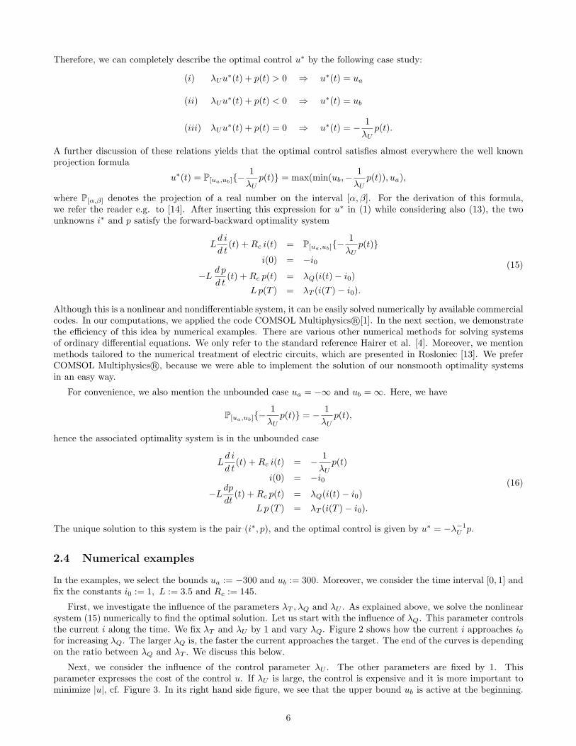
At first view, there are no significant differences to the other models. However, if we concentrate on the timeclose to t = 0, we see a nonlinear increase of the electrical current i. This is shown in Figure 14 by different λU .The behaviour of the control u is similar to the linear case. First, the control stays on the upper bound and nextit decays to the holding level, see Figure 17.

Now we consider the induction L. Because L depends on i, we need to analyse L only near the initial time. InFigure 15 we see how the induction increases up to the value 1 and grows up to the holding level. This is caused by

18

0.02 0.04 0.06 0.08 0.10

1.0

0.5

0.0

0.5

1.0i [A]

t [s]

λU = 10−6

λU = 10−4

λU = 1

-

-

Figure 14: Electrical current i by different λU

0.02 0.04 0.06 0.08 0.10

1

2

3

4

5

6

7i [A]

t [s]

λU = 10−6

λU = 10−4

λU = 1

Figure 15: Induction L by different λU

the fact that i is starting at −i0 = −1. At the value i(t) = 0, the induction must be equal to L(0) = a+ b · 02 = 1and admit a minimum there. After that point, the induction grows again up to a holding level.

Finally, we compare the case with constant induction of Model 1 ( cf. 2.4 ) and with the last model with timedependent induction. We use the same parameters as before. In Figure 16 we can see the differences in the statei. With constant induction, the electrical current i grows smoothly. In the case with time dependent induction L,the current grows slower at the beginning. After some short time, the current increases faster than by constantinduction and reaches earlier the value of i0. In Figure 17, the curves of the controls u are plotted. Here we can see

0.02 0.04 0.06 0.08 0.10

1.0

0.5

0.5

1.0

i [A]

t[s]

constant inductionlinear induction

-

-

0.005 0.010 0.015 0.020 0.025 0.030

1.0

0.5

0.0

0.5

1.0

i [A]

t [s]

constant inductionlinear induction

-

-

Figure 16: Comparison of the electrical current by different inductions

that in the case with constant induction the control stays longer at the upper bound. However, both curves havethe same characteristic behaviour.

The computational time for solving the nonlinear optimal control problem is about 850 seconds (Single Core 3GHz,4 GB RAM) in contrast to the linear problem of Section 2.4 with about 180 seconds.

19

0.000 0.005 0.010 0.015 0.020 0.025 0.0300

50

100

150

200

250

300

u [V]

t [s]

constant induction

linear induction

Figure 17: Comparison of the voltage by different inductions

Remark 5. By our numerical method, we just solve the first-order optimality system. This system of necessaryconditions is not sufficient for local optimality, if a nonlinear state equation models the electric current. Howevercomparing the results for the nonlinear equation with those for the linear one, we can be sure to have computed theminimum. Another hint on optimality is that the current reaches the desired state in short time.

Conclusions. We have considered a class of optimal control problems related to the control of electric circuits.It is shown that, by an approiate choice of parameters, the time optimal transfer of an initial state to another onecan be reduced to a fixed time control problem with quadratic objective functional. Invoking the kown theory offirst-order necessary optimality conditions, a non-smooth optimality system is set up, which can be directly solvedby available software for differential equations. This direct and slightly non-standard numerical approach turnedout to be very efficient and robust for this class of optimal control problems.

20

References

[1] Software COMSOL Multiphysics R©. internet reference: www.comsol.com.

[2] M. Athans and P. L. Falb. Optimal control. An introduction to the theory and its applications. McGraw-HillBook Co., New York, 1966.

[3] G. Feichtinger and R. F. Hartl. Optimale Kontrolle okonomischer Prozesse. Walter de Gruyter & Co., Berlin,1986. Anwendungen des Maximumprinzips in den Wirtschaftswissenschaften.

[4] E. Hairer, S. P. Nørsett, and G. Wanner. Solving ordinary differential equations. I, Nonstiff problems, volume 8of Springer Series in Computational Mathematics. Springer-Verlag, Berlin, second edition, 1993.

[5] R. F. Hartl, S. P. Sethi, and R. G. Vickson. A survey of the maximum principles for optimal control problemswith state constraints. SIAM Rev., 37(2):181–218, 1995.

[6] A. D. Ioffe and V. M. Tihomirov. Theory of extremal problems, volume 6 of Studies in Mathematics and itsApplications. North-Holland Publishing Co., Amsterdam, 1979.

[7] J. Jahn. Introduction to the Theory of Nonlinear Optimization. Springer-Verlag, Berlin, 1994.

[8] D. G. Luenberger. Optimization by Vector Space Methods. Wiley, New York, 1969.

[9] J. W. Macki and A. Strauss. Introduction to optimal control theory. Springer-Verlag, New York, 1982. Under-graduate Texts in Mathematics.

[10] I. Neitzel, U. Prufert, and T. Slawig. Strategies for time-dependent PDE control with inequality constraintsusing an integrated modeling and simulation environment. Numer. Algorithms, 50(3):241–269, 2009.

[11] E. R. Pinch. Optimal Control and the Calculus of Variations. Oxford Science Publications, 1993.

[12] L. S. Pontryagin, V. G. Boltyanskii, R. V. Gamkrelidze, and E. F. Mishchenko. The mathematical theory ofoptimal processes. A Pergamon Press Book. The Macmillan Co., New York, 1964.

[13] StanisÃlaw RosÃloniec. Fundamental Numerical Methods for Electrical Engineering. Springer Publishing Com-pany, Incorporated, 2008.

[14] F. Troltzsch. Optimal Control of Partial Differential Equations. Theory, Methods and Applications. GraduateStudies in Mathematics, Volume 112. American Mathematical Society, Providence, 2010.

21