JOURNAL OF COMPUTATIONAL AND APPUED MATHEMATICS

ELSEVIER Journal of Computational and Applied Mathematics 83 (1997) 39-54

On spline regularized inversion of noisy Laplace transforms M. Iqbal*

Department of Mathematical Sciences, Kin9 Fahd University of Petroleum and Minerals Dhahran 31261, Saudi Arabia

Received 28 June 1995; received in revised form 31 January 1997

Abstract

In this paper we have converted the Laplace transform to an integral equation of the first kind of convolution type, which is an ill-posed problem and used the spline regularization method to solve it. Inversion of perturbed Laplace transforms also plays an important role in system theory. The method is applied to several test examples taken from [1-3, 8, 11, 22]. It gives a good approximation to the true solution and compares well with the methods discussed in [1-3, 8, 11, 22]. The results are shown in Table 1 and respective diagrams.

Keywords." Inversion of Laplace transform; Ill-posed problem; Convolution equation; Cross-validation; Spline regularization; Filter function; System theory

AMS classification: 65R20; 65R30

1. Introduction

Noisy Laplace transforms arise in a wide variety of practical problems. It is frequently used in system theory and linear dynamical systems. It is also used in statistics where a sample is drawn from a cumulative distribution function G, which is an unknown mixture of exponential distributions and hence can be written as

/0 G ( t ) = (1-e-St)f(s)ds, tE(O, ec),

where f is a probability density function with support in (0, oo). Ostrowsky et al. [13] introduced the exponential sampling technique for inversion of the Laplace

transform in photon correlation spectroscopy. There are many problems whose solution may be found in t e rms o f a Lap lace t r a n s f o r m which , howeve r , is too c o m p l i c a t e d for invers ion us ing different me thods . H o w e v e r , no s ingle m e t h o d g ives o p t i m u m resul ts for all pu rposes and all occas ions .

* E-mail: Internet facl 126@saupmoo Bitnet.

0377-0427/97/$17.00 @ 1997 Elsevier Science B.V. All rights reserved PII S 03 7 7 - 0 4 2 7 ( 9 7 ) 0 0 0 2 8 - 9

40 M. lqballJournal of Computational and Applied Mathematics 83 (1997) 39-54

For a detailed bibliography, the reader should consult Piessens [16] and Piessens and Branders [17]. The problem is of the recovery of a real function f ( t ) , t >~ O, given its Laplace transform

fo ~ = g(s) (1.1) e-St f ( t ) d t

for real values of s. The Laplace transform inversion is an ill-posed problem and, therefore, affected by numerical

instability. The ill-posedness of Laplace transform inversion in the case where f E L2(~+) and g(s) is known for all real and positive values of s, can be investigated by means of the Melline transform [11]. In practice, however, g(s) is known only in a finite set of points. The case of an infinite set of equidistant points was investigated by Papoulis [14]. Several methods and a comparison is given in [5, 20].

The previous methods do not include regularization techniques. Regularization methods have been discussed by Varah [22], Essah and Delves [6], Chauveau [3] and Brianzi [2]. Regularization by means of truncated singular function expansion is investigated by Brianzi in [2]. Other methods are also available in the literature for the numerical evaluation of the Laplace transform inversion which have been described by Linz [10], Norden [12] and Salzer [18]. A maximum likelihood approach is establishd by Jewell [9].

2. Description of the method

In (1.1) given g(s), s ~ O , we wish to find f ( t ) for t ~ 0 and f ( t ) = O for t<O, so that (1.1) holds. Frequently, g(s) is measured at certain points. We assume g(s) is given analytically with known f ( t ) , so that we can measure the error in the numerical solution. In order to convert the Laplace transform into the first kind integral equation of convolution type, we make the following subsitution in Eq. (1.1).

s = a x and t = a -y where a > l . (2.1)

Then

/5 o(a x) = ( log a)e-~-" f ( a - Y ) a -y dy. (2.2)

Multiplying both sides of (2.2) by a x we obtain the convolution equation

_~ K(x - y ) F ( y ) d y = G(x), - o c <~x <~ e~, (2.3)

where

G(x) = aX g(a x) = so(s),

K(x) = ( log a)aXe -~ = ( log a)s e -s, (2.4)

F ( y ) = f ( a -y) = f ( t ) .

M. Iqbal l Journal of Computational and Applied Mathematics 83 (1997) 39-54 41

In order that we can apply our deconvolution method to Eq. (2.3), it is necessary that G(x) has essentially compact support, i.e. G(x)-+O as x -+ -4-c~ or 12 - a ( x ) ] ---, 0 as x---, + c ~ , where ). = maxlG(x)l as x - + +c~ which is a property, we demand from our data function G(x).

2.1. Tikhonov reyularization usin9 cardinal cubic B-splines

Let Bj(H;x) be the Nth-order cardinal B-spline (N even) with knotes ( j - ½N),.. . , ( j + ½N)H, 1 i.e. Bj(H;x) = QN(~ - j + ~N), where

1 ( 7 ) ,,+ O u ( x ) - ( X - 1)! ~--~(-11/ ( x - " N--I j=0

In addition, let M H = T where M ~<N is an integral power of 2. We assume that Bj(H;x) is periodically continued outside the interval (0, T) with period T. Then Bj(H,x) has a Fourier series

o~ Bj(H;x)= ~ Bjqexp(ia~qX), (2.6)

q~-(x3

where

/0 T Bjq = B j ( H ; x ) exp(- iOgqX) (2 .7 )

and ~Oq = 2xq/T. Since B/(H;x) is simply a translation of Bo(H;x) by an amount jH, we have

/~jq =/~0,q exp(-icoqH),

where

H [sin(ogqH/2) 4 /~0,q = L ~ (2 .8 )

Now we shall approximate the convolution Eq. (2.3) by

o r KN(x -- y)FM(y) dy = Gu(x), (2.9)

where we assume that F, G and K have essentially finite support in [0, T), FM is a cubic spline (N = 4 ) of the form

M--I FM(x)= ~ ~jB/(H;x), M<.N. (2.10)

j=l

The real M-dimensional vector

~X = (0~0, ~1 , . - - , ~M--1)T

of unknown coefficients needs to be determined.

42 M. Iqbal/Journal of Computational and Applied Mathematics 83 (1997) 39-54

The spline in Eq. (2.10) has the Fourier series

FM(X) = ~ FM, q exp(iogqX), q=--oc

where M--1

PM, q~---- Z ~zjBjq j=0

(2.11)

M--1 ( 2xi . "~ =B0,q Z ~jexp - - - ~ j q )

j=0

7--- v/--MBo, q~s, s =-- q(modM). (2.12)

Here

_~ = ~/~_~, (2.13)

where the symbol 'H' denotes the Hermitian transpose. We find it advantageous to determine _~ rather than ~, because of the simple properties available

in discrete Fourier spaces. The vector _~ in Eq. (2.10) may then be determined from the inverse M-dimensional fast Fourier transform (FFT)

_~= OMc2, (2.14)

where ~p is the unitary matrix with elements

1 [2xi "~ q, rs v ~ -- e x p ~ - r s ) , r , s=O, 1 , 2 , . . . , N - 1 .

2.2. Pth-order Tikhonov regularization [21]

Consider the smoothing functional

C(FM; ,~ ) = C(_~,,~) = IIKN * FM -- Gull~ + ,~IIFM~P~II~,

where F(M e) is the pth order derivative. Using Plancherel's theorem we have

1 u/2 -- GN, ql . IIKN * FM - - GNII~ = ~ ~ ]KN, qPM, q ^ 2

q:--N/2

Hence, using Eq. (2.12) we have

1 1/2N [[KN * FM -- GNII~ = -~i Y~ [(x//MJ~o,qRN, q ~s -- ON, q)(V/-'MB°,qKN, q~s - ~N,q)],

q=-- 1/2N

(2.15)

(2.16)

where s - q (modM).

M. lqbal l Journal of Computational and Applied Mathematics 83 (1997) 39-54 43

Also, Plancherel's theorem applied to the regularizing functional in Eq. (2.15) gives

[[FM(P)[[ : ~ (D~PIPM, q[ 2 = 2 E ('Oq 2pIpM,ql2 q=--oo q=l

2p^2 ^ 2 = 2M (9q Bo, q[O~s[ , where s - q ( m o d m ) . (2.17) q=l

The simplification of expression (2.17) requires the use of an attenuation factor %. For cubic cardinal splines it is shown by Stoer [19] and Gautschi [7] that

sin(xq/M)- 4 3 Tq = TCq/M 1 + 2COS(TCq/M)" (2.18)

In expression (2.17) we wish to arrange the summation over q to summation over s, where s = q (modM).

Define the matrix

[ d i a g ( v / - M B o , , K N , s ) ] o r d e r N x M , W (1) . . . . . . . . . . . . . (2.19)

[diag ( v ~ /~O,M-~ ~NM-~)J s = O , 1 . . . , M - 1 .

From the property Ku, q =-kN, N-q of discrete FTs, it then follows that expression (2.16) simplifies to

IlK * FM -- GNII~ = II w(1)_~- 0NIl 2 (2.20)

and (2.17) can be written as

} M--I 12 ,2p /~2 HF(P)[[ 2 = 2M ~ a~ Y~ ~M,+,~"O.M,+~

s=l n=0

M--1 = 2M ~ zs[&,l 2, (2.21)

s=l

where

T s = t ~ M n + s ~ O , M n + s

n=0

o~ [sin ~(Mn + s)/M] = ( 2 x ) 2p ~'~ (Mn + s)2p H 2 [ x(Mn + s)/M J ' (2.22)

n=O

"Cs = (2x)2PH2s 8 [sin(ns/M)] 8 o~ rts/M J E (Mn + s) 2p-8.

n=O

o(3 = (2~)2ps8JB20, s ~_,(Mn + S) 2p-8. (2.23)

n=O

44 M. lqbal l Journal of Computational and Applied Mathematics 83 (1997) 39-54

Since Ss = eM-~, Eq. (2.21) further simplifies to

]/2M

s=l

In particular, when p = 2 (the order of regularization) from (2.23), it follows that

Zs = (2g)4S4/~2 's Mn-+ s ) n=0

while

ZM_s=(R~)4s4B2os(Mt~S-__s) 4

so that

Zs -+- ZM-s=(21r')4s4B2's ~-~ Mn-+ s n~--o0

=- (2rQ4S4/~,s[1 q- 2 cos2(rts/M)] (see Pennisi [15]), 3 [sin ~s /M/~s /M] 4

Defining the M × M matrix

W (2) = diag{[M(z, + "cM-s )]l/: },

it follows from (2.24) that

IIg~.)ll~ _-II w(:)_~ll 2

Thus, from Eqs. (2.20) and (2.27) we may express the smoothing functional (2.15) as

c(_~, x ) = IIW"C~- dNIl~ + Xll W(2)-~ll~.

The minimizer of (2.28) is clearly

_~ = (W + ,W) -1W¢1)H~N,

where

W ~- W (1)HW(1)

V = W (:~ W (:).

(2.24)

(2.25)

(2.26)

(2.27)

(2.28)

(2.29)

(2.30)

M. lqbal/ Journal of Computational and Applied Mathematics 83 (1997) 39-54 45

It is not necessary to invert the matrix W + 2V directly because it is diagonal. From Eqs. (2.19), (2.26), (2.29) and (2.30), it follows that

- - "X"

1 ~o ~k~O~.~ + &M-,&M-,G~,M+, ~" = V ~ [~L{IRN,,I 2 + (s/(M - - s))81R~,M_~I= } + N22(~s + "CM-~)]'

1 /~0,st~N, s0N, s + (s/(M - S))4RN.M's~N,M_s] &s - ~ ^2 ^ 2 _ , (2.31)

Bo,,[IKN,~I + (s/(g S))"I&M-slq +N2,~(~ + ~,,,-s)

since

// " ~ S 4 ^

= (,Mn----~) Bo,~ (2.32)

we can easily verify that c2s = a~M_s SO that inverse FFT gives c¢ = OM_~ is a real vector as required.

2.3. The filter for cardinal B-Spline regularization

The Fourier coefficients of the regularized (filtered) solution FM EBM(0, T) clearly depends on 2 through Eqs. (2.12),(2.13) and (2.31). In Eq. (2.31), we denote the dependence of as on 2 by writing ~ = ~,(2). Thus, the Fourier coefficients of the filtered solution are

PM, q ( ,~ ) = v / - M B 0 , q ~ s ( / ~ ) , s ~ q (modM) ,

whereas those of the unregularized (unfiltered) solution is

FM, q(0) = ~/}0,qC2s(0).

Clearly, the underlying filter Zq;~ must satisfy

PM, q( ~ ) = Zq;2PM, q( O )

so that we can deduce

as(2) (2.33) zq,~- aX0)'

^2 ^ 2 B&[IKN, sl + (s/(Mn - s))81RN, M_slq Zq;s= ^2 R 2 ( s / ( g n s))~lk~,M_,lq+N=;~(~,+~,_A (2.34) ~,,[r N,~I +

The filter will, of course, apply to every Fourier coefficients q = 0, 4-1, + 2 , . . . , but will have only M possible values depending upon q modulo M. The regularization parameter 2 is still to be determined.

2.4. Determination o f regularization parameter 2

tp 2 Let the filtered solution FM E BM(O, T), which minimizes IIKN * F M - - GNII, ~ + ,ZlIF~II2 be given by (we have p = 2)

o()

FM(X) = E fM, q exp(iOOqX). ( 2 . 3 5 ) q = - o o

46 M. lqballJournal of Computational and Applied Mathematics 83 (1997) 39-54

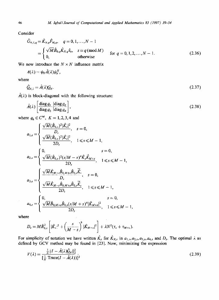
Consider

ON, 2,q~-RN, qPM, q, q ~ 0 , l . . . . , N - - 1

: f v/-MBo, qgN, q ~s, s=_q(modM)

t 0, otherwise

We now introduce the N × N influence matrix

A(2) = C N d ( 2 ) ~ ,

where

_ N2 A(2) is block-diagonal with the following structure:

.~(2) [ diaga' ]diaga2 ] diaga 3 ]diaga_4 '

where a_k E C M, K = 1,2, 3, 4 and

S ~ 0 , Os

al,~ -- v~ (&, s ) = lRs l ~ l < s < . M - 1, 2D~

0, s = 0,

az,s = v/--M(B°'s)2(s/M - - s)4Ks~M+s 1 <.S <.M -- l, 2D~

S : 0 , Os

a3,s= v~k~,+,ho,,,+sh0,,£'s l < s < . M - 1 , 2Ds

0, s = 0,

a4's= ~h° 'M+'B° ' s ( s /M + s)4[I(M+sl2 l <~s<~M- 1, 2D~

for q = 0, 1 , 2 , . . . , N - 1. (2.36)

(2.37)

(2.38)

where

Ds=MBo2,s I/(s[2+ ~ IKM-sl 2 + 2N2(zs + ZM+s).

For simplicity of notation we have written Ks for KN, s in al,s, a2,s, a3,s, a4,~ and D~. The optimal 2 as defined by GCV method may be found in [23]. Now, minimizing the expression

[~ Trace( / - 2(4))] 2 (2.39)

M. Iqbal l Journal of Computational and Applied Mathematics 83 (1997) 39-54 47

which from Eq. (2.38) can be written as

l {~sM__o 1 [ ( 1 - a l , s ) a s - a:,s~-s[: + ~sM=o ' I(1- a 4 , s ) G - s - a3,s412 } V(~) = N ( 2 A 0 ) 1 M--I [1 - ~ ~]s=o (al,s + a4,s)] 2

In order to minimize V(2) in Eq. (2.40), we have used a subroutine which uses a quadratic inter- polation technique to obtain a minimum.

3. Addition of random noise to the data functions

In solving the problems (1-5) , we have considered the data functions contaminated by varying amounts of random noise. To generate sequences of random errors of the form 8,, n = 0, 1 ,2 , . . . , N - 1, we have used a subroutine which returns pseudo-random real numbers taken from a normal distribution of prescribed mean A and standard deviation B.

To mimic experimental errors we have

A = 0 and B ( 1 - ~ ) = max [Gnl, (3.1) O<~n<~N--I

where X denotes a chosen percentage. In all our test problems we have taken X = 0.7 because Laplace transform is a severally ill-posed problem. Thus, the random error 5, added to Gn does not exceed 3X% of the maximum value of G(x).

4. Optimal convergence

Here we shall discuss the optimal convergence to the case of convolution equation (2.9).

o T X(x - y ) F ( y ) dy = G(x)

in which the function K is periodic of period T, expanding K in a Fourier series

/2 r6 _ y ) ) , K(x- y)= ~ I~oexp~--T-q(x q=-oo

where Kq is the Fourier coefficient, i.e.

o r {2=i "~ I~q = K ( y ) e x p ( - - f - q y ) d y = ~ u _ q .

We shall assume that

II~ql~_q-K, g>l

and so the Fourier series is uniformly convergent.

(4.1)

(4.2)

48 M. Iqbal/Journal of Computational and Applied Mathematics 83 (1997) 39-54

5. Test problems

Problem 1. This problem has been taken from [22].

9 ( s ) - 1/2 f ( t ) = 1 - e - t / 2 . s ( s + 1 /2 ) '

The optimal results are shown in Fig. 1, Table 1 and Varah's results in Fig. 6.

Problem 2. This problem has also been taken from [22].

2 9( s ) - f ( t ) = tZ e -t/2.

(s + 1/2)3'

The optimal results are shown in Fig. 2, Table 1 and Varah's results in Fig. 7.

Table 1

Test problem a T h 2 V(2) liE - Fx II ~ Fig.

1 10.0 9.60 0.150 0.31 x 10 -8 0.56358 0.01 1 2 15.0 12.10 0.18906 0.101 × 10 - l ° 0.6207 X 10 -8 0.015 2

3 10.0 11.60 0.18125 0.11 × 10 -8 0.1167 x 10 -8 0.010 3

4 10.0 12.20 0.19062 0.1009 × 10 -5 0.1411 × 102 0.070 4

5 8.0 12.60 0.19688 0.11 × 10 -8 0.1013 × 10 -9 0.007 5

1.00

0.80

0.60

S

0.40

0.20

~__Num~ noise 0.7%) soL(with

--*- Tree soln.

! I I I I I I I I I I

0 2 4 6 8 10 12 14 16 18 20 22

Fig. 1.

M. 1qball Journal of Computational and Applied Mathematics 83 (1997) 39-54 49

2.00

1.50

S ~'~ 1.00

0.50

[.4- Nun~soln.(with 0.7% noise)

I I i I I I I I I I I

2 4 6 8 10 12 14 16 18 20 22 t

Fig. 2.

0.400

0.350

0.300

0.250

--" 0.200

O. 150

0.100

0.050

0.000

0.00 0.20 0.40 0.60 0.80 1.00

I " True soln.

I I I I I I i I I I I I

1.41) 1.8O 2.20

Fig. 3.

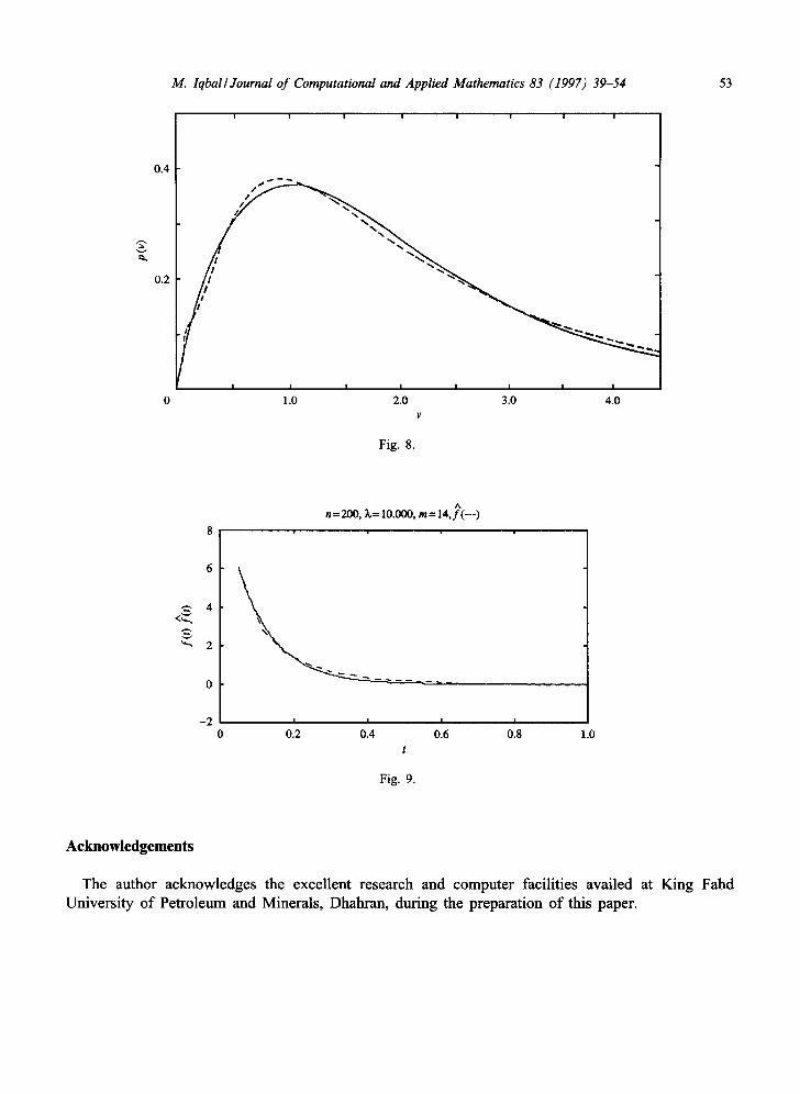
Problem 3. This problem has been taken from [11, 1, 2].

1 g ( s ) - - . . ~ , f ( t ) = te - t .

(s + 1)

The optimal results are shown in Fig. 3, Table 1 and McWhirter's results in Fig. 8.

50 M. Iqbal/Journal o f Computational and Applied Mathematics 83 (1997) 39-54

5

4

~ 3

2

1

0 | i ! ! !

0 0.20 0.40 0.60 0.80 1.00 t

4 Num. Soln.(with 0.7% noise) I

True Soln. [

, , 0 I I I

1.20 1.4t) • 1.61)

Fig. 4.

Problem 4. This problem has been taken from [3].

2 O(s) -- 2 + s '

f ( t ) = 2e -~t for 2 = 5.0.

The optimal results are shown in Fig. 4, Table 1 and Chauaveau's results in Fig. 9.

Problem 5. This problem has been taken from [4, 8], and we made the problem more ill-posed by taking higher value of ~ and adding noise.

g ( s ) = (s + ~)2 +/~2'

f ( t ) = e -s ' sin/~t for ~ = 3.0 and /~ = 1.0.

The optimal results are shown in Fig. 5 and Table 1.

6. Numerical results

In this section, we tabulate the results of the above method applied to the test problems taken from [1-3, 8, 11, 22]. All data functions have the property 9 ( s ) = 0(s -1) and 0.7% noise has been

M. IqballJournal of Computational and Applied Mathematics 83 (1997) 39-54 51

added apart from machine rounding error; only optimal results have been quoted in Table 1 and demonstrated in the respective diagrams. In each of the test problems, 64 sample points are used to calculate the discrete Fourier coefficients.

In our numerical calculations, we need to choose two numbers Xmi n and Xrnax- We find Xmi n and Xm~, as the smallest and largest solutions of the non-linear equation IG(x)l -- e where e = 10 -4. We may then pose the deconvolution problem (2.3) on the interval [0, T], where T = Xm~ - X m i n .

Since the size of the essential support of G(x) depends upon 'a ' , we have for a fixed number N of equidistant data points {xn}, h = TIN. We have minimized (2.40), which respect to 2 for values of a > 1 and compared the Loo error of the resulting solution with the values of the true solutions. We find the minimum value of V(2) which yields the Loo error of the regularized solution as the least.

7. Conclusions

Our method worked very well over all the test problems and the results obtained are shown in Figs. 1-5 and Table 1. As regards comparison with other available methods, the authors of the other methods obtained the results with clean data and we have added 0.7% noise in the data functions which make the problem more ill-posed. We have compared our results with others, i.e. with Varah [22], McWhirter and Pike [11], Brianzi [1, 2], and Chauveau [3], which are quoted in Figs. 6 -9 . The results of problem (5) are not available to compare with.

S

0.140

0.120

0.100

0.080

0.060

0.040

0.020

0.000

0.00

,••,•. [--~ Num.Soln.(with 0.7% noise)

-*- True Soln.

?

.

I I I I I I I I I I

0.10 0.20 0.30 0.40 0.50 0.60 0.70 0.80 0.90 1.00 t

Fig. 5.

52 M. 1qball Journal of Computational and Applied Mathematics 83 (1997) 39-54

1.44

1.22

1.00

0.78

0.56

0.34

0.12

-0.10

MLS(X=O.O01)

f(t)

ML$ (X=O.O1)

(~,=0.1)

I I I I I

2.326 6.977 11.628 t

MLS solutions for Example 2.

Fig. 6.

I !

16.279

3.118

2.641

2.165

1.689 S

1.212

0.736

0.260

-0.217

~ / M ~ (Z=IO -5)

/ ~ (Z=IO-s)

I I I I I I I

2.564 7.692 12.821 17.949 t

MLS solutions for Example 3. Fig. 7.

0.4

0.2

M. Iqbal/ Journal of Computational and Applied Mathematics 83 (1997) 39-54

i i i i i i i i

i j , ~' Z'

I I I I I I I I

1.0 2.0 3.0 4.0

Fig. 8.

53

A n =200, ~,= 10.000, m= 14,f(---)

0

- 2 0

. . . . " a - - -

I I I I

0.2 0.4 0.6 0.$ 1.0 t

Fig. 9.

Acknowledgements

The author acknowledges the excellent research and computer facilities availed at King Fahd University of Petroleum and Minerals, Dhahran, during the preparation of this paper.

54 M. lqbal/Journal of Computational and Applied Mathematics 83 (1997) 39-54

References

[1] P. Brianzi, A criterion for the choice of a sampling parameter in the problem of Laplace transform inversion, Inverse Problems 10 (1994) 55-61.

[2] P. Brianzi, M. Frontini, On the regularized inversion of the Laplace transform, Inverse Problems 7 (1991) 355-368. [3] D.E. Chauveau et al., Regularized inversion of noisy Laplace transforms, Adv. Appl. Math. 15 (1994) 186-201. [4] C. Cristina et al., Use of Laguerre functions in the inversion of Laplace transform, Inverse Problems 9 (1993)

57-68. [5] B. Davies, B. Martin, Numerical inversion of the Laplace transform, J. Comput. Phys. 33 (2) (1979) 1-32. [6] W.A. Essah, L.M. Delves, On the numerical inversion of the Laplace transform, Inverse Problems 4 (1988) 705-724. [7] W. Gautschi, Attenuation factors in practical Fourier analysis, Numer. Math. 18 (1972) 373-400. [8] G. Giunta et al., More on the Weeks method for the numerical inversion of the Laplace transform, Numer. Math.

54 (1988) 193-200. [9] N.P. Jewell, Mixtures of exponential distributions, Ann. Statist. 10 (1982) 479-484.

[10] P. Linz, A new numerical method for ill-posed problems, Inverse Problems 10 (1994) L1-L6. [11] J.G. McWhirter, E.R. Pike, On the numerical inversion of the Laplace transform and similar FI equations of the first

kind, J. Phys. A 11 (9) (1978) 1729-1745. [12] H.V. Nordan, Numerical inversion of Laplace transform, Acta Acad. Abo. 22 (1981) 3-31. [13] N. Ostrowski et al., Exponential sampling method for light scattering poly-disperity analysis, Optica Acta 28 (1981)

1059-1070. [14] A. Papoulis, A new method of inversion of Laplace transform, Quart. Appl. Maths. 14 (1956) 405-414. [15] L.L. Pennisi, Elements of Complex Variables, McGraw-Hill, New York, 1976. [16] R. Piessens, Laplace transform inversion, J. Comput. Appl. Math. 1 (1975) 115-128. [17] R. Piessens, M. Branders, Numerical inversion of the Laplace transform using generalized Laguerre polynomials,

Proc. IEE 118 (1971) 1517-1522. [18] H.E. Salzer, Orthogonal polynomials arising in the numerical evaluation of inverse Laplace transform, Math. Tables

and Other Aids to Comput. 9 (1955) 164-177; also J. Math. Phys. 37 (1958) 80-108. [19] J. Stoer, R. Bulirsch, Introduction to Numerical Analysis, Springer, Berlin (1978). [20] A. Talbot, The accurate numerical inversion of Laplace transforms, J. Inst. Math. Appl. 23 (1) (1979) 97-120. [21] A.N. Tikhonov, V.Y. Arsenin, Solution of ill-posed Problems (translated from the Russian), Wiley, New York, 1977. [22] J.M. Varah, Pitfalls in the numerical solution of linear ill-posed problems, SIAM J. Sci. Statist. Comput. 4 (2)

(1983) 164-176. [23] G. Wahba, Practical approximate solutions to linear operator equations when the data are noisy, SIAM J. Numer.

Anal. 14 (1977) 651-677.