Embed Size (px)
Citation preview

1/36Symposium to honor Bill Wolovich, December 2008, Cancun, MexicoHitay Özbay
On Strongly Stabilizing Controller Synthesis
Hitay ÖzbayBilkent University, Ankara Turkey
Symposium to Honor Bill WolovichCancun, Mexico, December 7, 2008

2/36Symposium to honor Bill Wolovich, December 2008, Cancun, MexicoHitay Özbay
OUTLINE
Definition of the Strong Stabilization Problem
MIMO Finite Dimensional Plants Case
A parameterization of strongly stabilizing controllers
An LMI based design for reduced conservatism
Strongly Stabilizing Controllers for Systems with Delays
PD-like Stable Controllers
Conclusions

3/36Symposium to honor Bill Wolovich, December 2008, Cancun, MexicoHitay Özbay
Strong Stabilization Problem
P(s)C(s)r e uc
vu y+
-++
We say that C strongly stabilizes P if (i) C is stable and (ii) the closed-loop system (C,P) is stable.
Why strong stabilization?• Simultaneous stabilization of two plants is equivalent to
strong stabilization of another plant.
• Robustness to sensor failures in the feedback path.
• The capability to test the stand-alone controller off-line.

4/36Symposium to honor Bill Wolovich, December 2008, Cancun, MexicoHitay Özbay
Strong stabilization Parity Interlacing Property (PIP) : For a given plant P, there exists a strongly stabilizing controller if and only if the number of poles of P (counted according to their McMillan degrees) betweenevery pair of real blocking zeros of P in the extended right half plane is even.
An iterative construction method for computing such a unit is given by Youla et al. (1974). Parameterization of all strongly stabilizing controllers is given by Vidyasagar (1985) using an interpolationapproach.
Controller Design (SISO Case):Let P = NM−1, where N,M ∈ H∞ are coprime factors,and zi, i = 1, . . . , ` denote the extended right half plane zeros of P .There exists a strongly stabilizing controller C⇐⇒there exists a unit U in H∞ satisfying U(zi) =M(zi) for i = 1, . . . , `.Moreover, a strongly stabilizing controller C is given by,
C =U −MN
.

5/36Symposium to honor Bill Wolovich, December 2008, Cancun, MexicoHitay Özbay
OUTLINE
Strong Stabilization Problem
MIMO Finite Dimensional Plants Case
A parameterization of strongly stabilizing controllers
An LMI based design for reduced conservatism
Strongly Stabilizing Controllers for Systems with Delays
PD-like Stable Controllers
Conclusions
6/36Symposium to honor Bill Wolovich, December 2008, Cancun, MexicoHitay Özbay
State Space Approach for MIMO Plants
G
K
wz
y u
∙MN
¸=
⎡⎣ AX | BF | IC | 0
⎤⎦ ∈ RH∞,with F = −BTX, and X = XT ≥ 0 being the solution of
ATX +XA−XBBTX = 0
so that AX := (A+BF ) is stable.
P (s) = G22(s) = C(sI −A)−1B = NM−1, where
Note that M is inner.
A coprime factorization (RCFND):
Assume (A,B) stabilizable, (C,A) detectable.
Assume G22 does not have poles on the Im-axis.

7/36Symposium to honor Bill Wolovich, December 2008, Cancun, MexicoHitay Özbay
So, if
infQ∈RH∞
k[F (sI −AX)−1B 0]−Q(s)[C(sI −AX)−1B1
ρI]k∞ < 1
then there exists a strongly stabilizing controllerfor some ρ > 0,ρ.
This is a two-block H∞ control problem and if it is solvable for some then it is solvable for all ρ ≥ ρo.
A stable controller K is strongly stabilizing if and only if
is a unit in
U =M +KN = I + F (sI −AX)−1B +K(s) C(sI − AX)−1B
RH∞.
whose norm is bounded by
ρ = ρo > 0,

8/36Symposium to honor Bill Wolovich, December 2008, Cancun, MexicoHitay Özbay
Zeren and Özbay (Automatica, 2000):There exists a strongly stabilizing stabilizing controller if
Moreover, when this condition holds, all controllers in the form given below with are strongly stabilizing:Q ∈ RH∞, kQk∞ < ρ
Q
Mo
K(s) A dual result can be obtained starting from a LCFND instead of a RCFND.
there exists ρ > 0 such that
AXY + Y ATX − Y (ρ2CTC −XBBTX)Y +BBT = 0
has a stabilizing positive definite solution, i.e. Y = Y T ≥ 0 with stable AX + LC.Under this sufficient condition, a stable controller K, with kKk∞ ≤ ρ, is given by
K = −F (sI −AK)−1L ; AK = (A+BF +LC), F = −BTX, L = −ρ2Y CT .
M0(s) =
⎡⎣ A+BF + LC | −L BF | 0 I−C | I 0
⎤⎦ .

9/36Symposium to honor Bill Wolovich, December 2008, Cancun, MexicoHitay Özbay
An LMI Based Design for Reduced Conservatism
There exists a strongly stabilizing controller, K with if there exist and Z satisfying the LMIs
kKk∞ ≤ γKXK = X
TK > 0
Gümüşsoy-Özbay (IEEE T-AC, 2005):
Let be as defined before.X and AX
Under the above sufficient condition a strongly stabilizing controller is given by
Reduces to Zeren-Özbay (2000) with

10/36Symposium to honor Bill Wolovich, December 2008, Cancun, MexicoHitay Özbay
Moreover, all controllers in the set
and
are strongly stabilizing, where
Q
KoG,ss
K(s)

11/36Symposium to honor Bill Wolovich, December 2008, Cancun, MexicoHitay Özbay
Stabilize G1 and G2 by stable controllers, K where |K|∞<γK using LMI-based result.Solve the same problem using Zeren-Özbay (2000), with |K|∞<ρmin.Compare γK and ρmin (comparison of conservatism)Note that for G1 as α 5 and for G2 as α 0, p.i.p. is close to being violated
Examples
LMI based approach
Zeren-Özbay

12/36Symposium to honor Bill Wolovich, December 2008, Cancun, MexicoHitay Özbay
OUTLINE
Strong Stabilization Problem
MIMO Finite Dimensional Plants Case
A parameterization of strongly stabilizing controllers
An LMI based design for reduced conservatism
Strongly Stabilizing Controllers for Systems with Delays
PD-like Stable Controllers
Conclusions

13/36Symposium to honor Bill Wolovich, December 2008, Cancun, MexicoHitay Özbay
Strongly Stabilizing Controllers for Systems with Time Delays
P (s) =(s− 2)e−τs
(s+ a− ke−hs)
"1s+1
1s+2
1s+3
0 0 e−2τs
s+4+e−s
#
Özbay (IFAC 2008): Zeren-Özbay approach can be extended to plants of the form
a, h, k, τ > 0 with kh < 1 and k > a.
The plant contains a single pole in C+This pole, denoted by α, is the unique solution of α = ke−hα − a.
{2,∞}Blocking zeros in the extended right half plane:
The plant satisfies the PIP if and only if α < 2.
P = D−1p Np, where Dp, Np ∈ H∞ strongly coprime, and Np(s) = Npi(s)Npo(s)Np1(s)
is finite dimensionalDp
is right invertible in H∞.
Npiwith inner, Npo outer finite dimensional, and
Np1
Example:

14/36Symposium to honor Bill Wolovich, December 2008, Cancun, MexicoHitay Özbay
Npi(s) =(s− 2)(s+ 2)
e−τs∙1 00 e−2τs
¸Npo(s) =
1
s+ 1I
Np1(s) =(s− α)
(s+ a− ke−hs)
∙s+2s+1 1 s+2
s+3
0 0 s+2s+4+e−s
¸
N†p1(s) =
(s+ a− ke−hs)(s− α)
⎡⎣ 2 s+1s+2
0
−1 − s+4+e−ss+3
0 s+4+e−ss+2
⎤⎦
infq2∈H∞
k− (α+ 1)s+ 1
+(s− 2)
(s+ 2)(s+ 1)e−3τsq2(s)k∞ < 1
For the plant given here, we can find a strongly stabilizing controller using this approach if and only if
For the problem is solvable if and only if τ = 0 13 <
1α+1 ⇐⇒ α < 2
which is equivalent to PIP.

15/36Symposium to honor Bill Wolovich, December 2008, Cancun, MexicoHitay Özbay
For largest for which we can find a strongly stabilizing controller using this approach is shown in the figure.
τ > 0 α

16/36Symposium to honor Bill Wolovich, December 2008, Cancun, MexicoHitay Özbay
Sensitivity Minimization by Stable Controllers Gümüşsoy-Özbay (CDC2007, IEEE T-AC to appear)
P(s)C(s)r e uc
v
u y+-
++
Feedback system is stable if and only if S = (1 + PC)−1, PS and CS are in H∞
C ∈ H∞and stabilizes the feedback system with plant P then we say that it is a strongly stabilizing controller. The set of all strongly stabilizing controller for the plant P is denoted by S∞(P )
If a controller is stable, WSMSC: given W and P, find
γss = infC∈S∞(P)
kW (1 + PC)−1k∞,
= kW (1 + PCγss)−1k∞

17/36Symposium to honor Bill Wolovich, December 2008, Cancun, MexicoHitay Özbay
P (s) =mn(s)
md(s)No(s)
inner, finite dimensional
inner, possibly infinite dimensionalouter, possibly infinite dimensional
The Class of Plants Considered in This Section:
Examples from time delay systems will be given.

18/36Symposium to honor Bill Wolovich, December 2008, Cancun, MexicoHitay Özbay
Factorization of Unstable Time Delay Systems
P (s) =mn(s)
md(s)No(s)P (s) =
R(s)
T (s)=
Pni=1Ri(s)e
−hisPmj=1 Tj(s)e
−τjs
0 = h1 < . . . < hn 0 = τ1 < . . . < τm
Ri and Tj are finite dimensional stable proper functions with no Im-axis zeros.R(s) has finitely many zeros in the right half plane.T(s) may have infinitely many zeros in the right half plane.
Example: x(t) + 2x(t− 2) = −x(t) + 2x(t− 2) + u(t),y(t) = 4x(t− 3)− 2x(t− 2) + 2x(t− 2) + u(t)
P (s) =(s+ 1) + 4e−3s
(s+ 1) + 2(s− 1)e−2s =1e−0s +
³4s+1
´e−3s
1e−0s +³2(s−1)s+1
´e−2s
Assumption:

19/36Symposium to honor Bill Wolovich, December 2008, Cancun, MexicoHitay Özbay
Then is stable and minimum phase.R(s)
MR(s)
We can do the same for T when it has finitely many zeros in the right half plane.But in this paper we consider a more general case where T is allowed to have inifinitely many zeros in the right half plane.
Define the conjugate of T as T (s) := e−τmsT (−s)MC (s)where MC(s) is a finite dimensional inner function whose zeros are the poles of T.
T (s) is like R(s), it has finitely many zeros in the right laf plane.MT (s)Define a finite Blaschke product from these zeros, so that
MT
Tis outer. Then we have:
md =MT
T
T, mn =MR, No =
R
MR
MT
T.P (s) =
mn(s)
md(s)No(s)
Let be the zeros of R(s) in the right half plane.s1, . . . , snr
Define an inner function MR(finite Blaschke product) from s1, . . . , snr

20/36Symposium to honor Bill Wolovich, December 2008, Cancun, MexicoHitay Özbay
Example:
Zeros of R(s) in the right half plane: 0.3125± j0.8548
T (s) = 2 +
µs− 1s+ 1
¶e−2s it has no zeros in the right half plane.
R(s) = 1 +4
s+ 1e−3s T (s) = 1 + 2
(s− 1)(s+ 1)
e−2s
md(s) =T (s)
T (s),
mn(s) = MR(s) =s2 − 0.6250s+ 0.8283s2 + 0.6250s+ 0.8283
,
No(s) =R(s)
MR(s)
1
T (s).

21/36Symposium to honor Bill Wolovich, December 2008, Cancun, MexicoHitay Özbay
Interpolation Approach for the Solution of WSMSC
WSMSC: given W and P, find
WLet be minimum phase
P (s) =mn(s)
md(s)No(s)
s1, . . . , sN zeros of mn C+in
Once such an F is found the corresponding the stable controller is
Cγ =(W − γ md F )
γ mnN−1o F−1 ∈ H∞
if and only if there exists such that
Feedback system is stable and kW (1 + PC)−1k∞ ≤ γ
F ∈ H∞ F−1 ∈ H∞ and
F (si) =W (si)
γmd(si)=:
ωiγ, i = 1, . . . , N
γss = infC∈S∞(P)
kW (1 + PC)−1k∞,
= kW (1 + PCγss)−1k∞

22/36Symposium to honor Bill Wolovich, December 2008, Cancun, MexicoHitay Özbay
C+ Ds
zconformal map
z = ϕ(s) = s−as+a , a > 0
g(z) = G(ϕ−1(z))
zi = ϕ(si), i = 1, . . . ,N
Ganesh-Pearson (ACC, 1986) solution via the Nevanlinna-Pick interpolation:
F (s) = e−G(s) G(s) = − lnF (s)Find and analytic function G : C+ → C+ such that
mi ∈ Z
Optimal solution is the smallest such that the Pick matrix whose entries are given below is positive semidefinite:
(over all possible integers )mi,mk ∈ Z
Pi,k =2 ln γ − lnωi − ln ωk + j2πmk,i
1− zizkmk,i = mk −mi
γss γ
G(si) = − lnωi + ln γ − j2πmi =: νi

23/36Symposium to honor Bill Wolovich, December 2008, Cancun, MexicoHitay Özbay
Example
R(s) = 1 +4
s+ 1e−3s
T (s) = 1 + 2(s− 1)(s+ 1)
e−2smd(s) =
T (s)
T (s),
mn(s) = MR(s) =s2 − 0.625s+ 0.828s2 + 0.625s+ 0.828
.No(s) =R(s)
MR(s)
1
T (s).
Let W (s) =1 + 0.1s
1 + sthen ω1,2 = 0.79∓ j0.85
s1,2 = 0.31± j0.85
(computed from the 2x2 Pick matrix)
F (s) = e−0.57s
Resulting “optimal” interpolating function is
Clearly F−1 6= H∞ and the corresponding controller includes a time advance.
γss = 1.07

24/36Symposium to honor Bill Wolovich, December 2008, Cancun, MexicoHitay Özbay
kF−1k∞ ≤ ρNow we add an extra condition:
This also puts a bound on the H∞ norm of the controller:
kCγk∞ ≤ kNok−1∞µ1 +
ρ
γkWk∞
¶.
Recall that in the unrestricted problem we are looking for an F (s) = e−G(s)
for some analytic G : C+ → C+ satisfying G(si) = νi, i = 1, . . . , n.
0 < Re(G(s)) < ln(ρ) =: σo
In this case we have s ∈ C+for all
So we need
Modified Interpolation Problem
Cσo+ := {s ∈: 0 < Re(s) < σo}
and now we seek an analytic function
where
|F (s)−1| = |eRe(G(s))|
G : C+ → Cσo+ satisfying G(si) = νi, i = 1, . . . , n,
Define as the smallest γ for which a feasible solution exists.γss,ρ

25/36Symposium to honor Bill Wolovich, December 2008, Cancun, MexicoHitay Özbay
This problem can be solved by using Nevanlinna-Pick interpolation using the following conformal maps
z = φ(s) =s − 1s + 1
s = φ−1(z) =1 + z
1 − z
z = ψ(s) =je−jπs/σo − 1je−jπs/σo + 1
s = ψ−1(z) =σoπ
µπ
2+ j ln(
1 + z
1 − z )¶,

26/36Symposium to honor Bill Wolovich, December 2008, Cancun, MexicoHitay Özbay
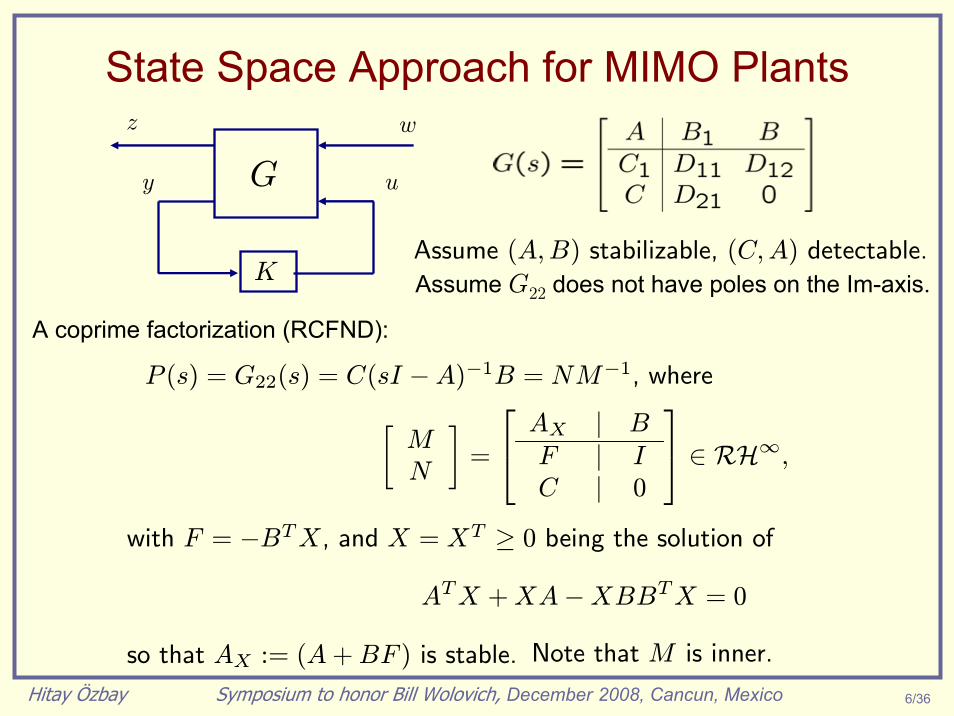
γss = 1.07
Back to the example:Recall that now as ρ→∞ we have γss,ρ → γss
But there is a lower bound on how small ρ can get: ρmin = e0.88 = 2.41
27/36Symposium to honor Bill Wolovich, December 2008, Cancun, MexicoHitay Özbay
G(s) := g(φ(s)) = j−0.99794(s− 3.415)(s+ 1)(s+ 3.406)(s+ 1.001)
.
ρ = e3 ≈ 20, we have γss,ρ = 1.08,For corresponding optimal interpolant is
F (s) = exp(−σo2− jσo
πln(1 + G(s)
1− G(s))).
which results in
This is an infinite dimensional transfer function whose rational approximations can be obtained.

28/36Symposium to honor Bill Wolovich, December 2008, Cancun, MexicoHitay Özbay
For γ = 1.08 we find a feasible suboptimal solution
kFk∞ =295.84
296.27< 1
F (si) =ωi1.08
, for i = 1, 2zero(F) = −50.9245,−2.2583± j 8.9628pole(F) = −3.3510,−1.4851± j 2.5881
F (s) =0.068s3 + 3.77s2 + 21.45s + 295.84
9.93s3 + 62.77s2 + 187.25s + 296.27.

29/36Symposium to honor Bill Wolovich, December 2008, Cancun, MexicoHitay Özbay
OUTLINE
Strong Stabilization Problem
MIMO Finite Dimensional Plants Case
A parameterization of strongly stabilizing controllers
An LMI based design for reduced conservatism
Strongly Stabilizing Controllers for Systems with Delays
PD-like Stable Controllers
Conclusions

30/36Symposium to honor Bill Wolovich, December 2008, Cancun, MexicoHitay Özbay
PD-like Controllers for MIMO Systems with DelaysGündeş-Özbay-Özgüler (Automatica 2007)
e u
v
+
−++
Gy
delays LTI-FD
Plant
PD Controller
Define
As a shorthand notation we will write
to represent all possibilities
delays
Λi Λo
Λ?(s) = diag£e−T
?1 s, · · · , e−T?r s
¤
GΛ
T ?j ∈ Θ?j = [0 , T j?max) ⊂ R+
T ? := (T ?1 , . . . , T ?r ) and Θ? := (Θ?1, . . . ,Θ?r)
T ?j ∈ Θ?j , 1 ≤ j ≤ r
yref
(T i, T o) = T ∈ Θ = (Θi,Θo)
Cpd = Kp +Kd s
τds+ 1
very special stable controllerG(s) = C(sI − A)−1B +D
Cpd

31/36Symposium to honor Bill Wolovich, December 2008, Cancun, MexicoHitay Özbay
Consider plants G(s) with “single unstable pole” p≥ 0, and define coprime factors as follows:
Let rankG(s) = r, and let X(s) =(s− p)as+ 1
G(s) be stable for a > 0.
Assume rankX(p) = rank(s− p)G(s)|s=p = r, and
let X(0) = (s − p)G(s)|s=0 be nonsingular, G−1(0) = −pX(0)−1.
Further Structural Assumption:Y is diagonal, and hence G = Y −1X , X,Y ∈ H∞
GΛ = Y−1XΛ XΛ = ΛoXΛi

32/36Symposium to honor Bill Wolovich, December 2008, Cancun, MexicoHitay Özbay
Choose any bKd ∈ Rr×r, τd > 0. DefinebCpd(s) := X(0)−1 + bKd sτds + 1
ΦΛ :=(s− p)GΛ(s) bCpd(s)− I
s, eΦΛ := bCpd(s)(s − p)GΛ(s)− I
s.
If
0 ≤ p < max{minT ∈Θ
kΦΛk−1,minT ∈ΘkeΦΛk−1} =: φ,
then for any positive α ∈ R satisfyingp < α + p < φ
a PD-controller that stabilizes GΛ for all T ∈ Θ is given by
C pd(s) = (α + p ) bCpd(s).If bKd = 0, above is a P-controller.
PD-like controller synthesis:
33/36Symposium to honor Bill Wolovich, December 2008, Cancun, MexicoHitay Özbay
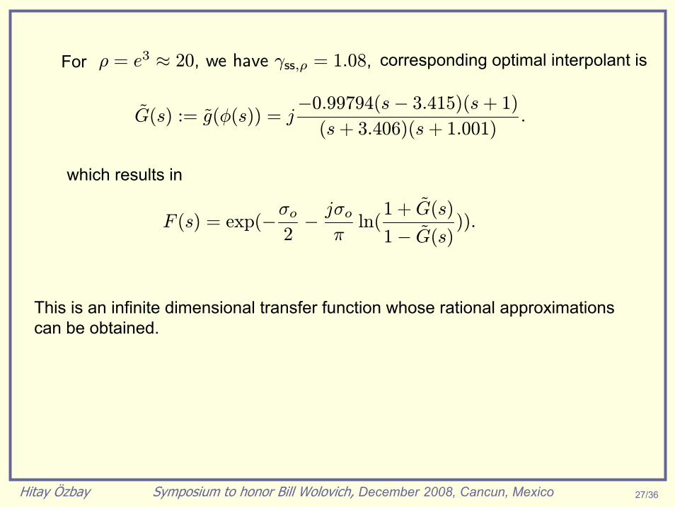
Example: Consider G(s) = 1s Go G1(s) with
Go =
∙3.04 −278.2/1800.052 206.6/180
¸G1(s) =
∙1 00 180
(s+6)(s+30)
¸.
An LCF of the plant is G(s) = Y (s)−1X(s), with
X(s) =1
as+ 1GoG1(s) Y (s) =
s
as+ 1I, a > 0.
Assume that the delays in the input channels are h1 and h2, and consider P control.
h2
h1
kΦΛk−1 Largest value = 4.86, for h1=0.18 and h2=0
For h2 = 0 and h1 > 0.2 we find αmax =1h1
Actual largest allowable gain is π2h1.
keΦΛk−1 = 1/max{h1, 0.2 + h2} = 5for h2 = 0 and 0 ≤ h1 ≤ 0.2.So, αmax = 5.

34/36Symposium to honor Bill Wolovich, December 2008, Cancun, MexicoHitay Özbay
Now consider the PD-controller α(I + Kd sτds+1
)G−1o where Kd =: KdG−1o .
The optimal Kd = KdG−1o is the one which minimizes kΦΛk.
Since ΦΛ is diagonal, we restrict Kd to be in the form diag(Kd,1,Kd,2).

35/36Symposium to honor Bill Wolovich, December 2008, Cancun, MexicoHitay Özbay
ConclusionsStrongly stabilizing controllers are obtained using a special factorization of the MIMO plants.Further optimization (e.g. H∞ and H2) in the paramaterized family of strongly stabilizing controllers is possible.An LMI-based technique reduces conservatism in this approach.The method can be extended to systems with time delays.Nevanlinna-Pick interpolation can be used for sensitivity minimization in the set of all strongly stabilizing controllers.PD- like controllers can be derived for MIMO plants with restricted number of poles in the right half plane (input/output delays are allowed in the plant).

36/36Symposium to honor Bill Wolovich, December 2008, Cancun, MexicoHitay Özbay
S. Gumussoy and H. Özbay, “Sensitivity Minimization by Strongly Stabilizing Controllers for a Class of Unstable Time-Delay Systems,” IEEE Transactions on Automatic Control, vol. 53, no. 12, December 2008, to appear. See also Proc. of the 46th IEEE Conference on Decision and Control, New Orleans, LA, December 2007, pp. 6071—6076.
A. N. Gündeş, H. Özbay, A. B. Özgüler, “PID controller synthesis for a class of unstable MIMO plants with I/O delays”, Automatica, vol. 43, No. 1, January 2007, pp. 135—142.
S. Gumussoy and H. Özbay, “Remarks on strong stabilization and stable H∞ controller design,” IEEE Transactions on Automatic Control, vol. 50, No. 12, December 2005, pp. 2083—2087.
M. Zeren and H. Özbay, “On the strong stabilization and stable H∞ controller design problems for MIMO systems,” Automatica, vol. 36 (2000), no. 11, pp. 1675–1684.
H. Özbay, “On Strongly Stabilizing Controller Synthesis for Time Delay Systems,”Proc. of the 17th IFAC World Congress, Seoul, Korea, July 2008, pp. 6342—6346.
The results presented in this talk are taken from the following papers:
Ackowledgements:
I would like to thank my co-authors for their contributions: Suat Gümüşsoy, Nazlı Gündeş, Bülent Özgüler, Murat Zeren