On Testing Global Optimization Algorithms for Space

On Testing Global Optimization Algorithms for Space

Trajectory Design

M. Vasile∗ and E. Minisci †

University of Glasgow, Glasgow, G12 8QQ, United Kingdom

M. Locatelli‡

Universita degli Studi di Torino, Turin, 10149, Italy

In this paper we discuss the procedures to test a global search algorithm applied to aspace trajectory design problem. Then, we present some performance indexes that canbe used to evaluate the effectiveness of global optimization algorithms. The performanceindexes are then compared highlighting the actual significance of each one of them. Anumber of global optimization algorithms are tested on four typical space trajectory de-sign problems. From the results of the proposed testing procedure we infer for each pairalgorithm-problem the relation between the heuristics implemented in the solution algo-rithm and the main characteristics of the problem under investigation. From this analysiswe derive a novel interpretation of some evolutionary heuristics, based on dynamical systemtheory and we significantly improve the performance of one of the tested algorithms.

I. Introduction

In the last decade many authors have used global optimization techniques to find optimal solutions to spacetrajectory design problems. Many different methods have been proposed and tested on a variety of cases.From pure Genetic Algorithms1–4 to Evolutionary Strategies (such as Differential Evolution)5 to hybridmethods,8 the general intent is to improve over the pure grid or enumerative search. Sometimes, the actualadvantage of using a global method is difficult to appreciate, in particular when stochastic based techniquesare used. In fact, if, on one hand, a stochastic search provides a non-zero probability to find an optimalsolution even with a small number of function evaluations, on the other hand, the repeatability of the resultand therefore the reliability of the method can be questionable. The first actual assessment of the suitabilityof global optimization methods to the solution of space trajectory design problems can be found in twostudies by the University of Reading7 and by the University of Glasgow.6 The former presented a small setof test problems mainly focusing on multiple gravity assist trajectories, while the latter included results forlow-thrust transfers using a wide range of global optimizers. One of the interesting outcomes of both studieswas that Differential Evolution, belonging to a subclass of Evolutionary Algorithms, performed particularlywell on most of the problems, compared to other methods. In both studies, the indexes of performancefor stochastic methods were: the average value of the best solution found for each run over a number ofindependent runs, the corresponding variance and the best value from all the runs. For deterministic methods,the index of performance was the best value for a given number of function evaluations. It should be notedthat the application of global methods to space trajectory problems has often considered the problem asa black-box with limited exploitation of problem characteristics. On the other hand, ad hoc techniquesexploiting problem characteristics7 provide a sensible improvement over the simple enumerative search.In this paper, we propose a testing methodology for global optimization methods addressing specificallyblack-box problems in space trajectory design. In particular, we focus our attention on stochastic basedapproaches. The paper discusses the actual significance of some performance indexes and proposes somecriteria to evaluate the actual usefulness of an algorithm. Furthermore, the paper presents a benchmark of

∗Senior Lecturer, Aerospace Engineering, James Watt South Building, AIAA Member.†Research Fellow, Aerospace Engineering, James Watt South Building.‡Associate Professor, Dipartimento di Informatica, Corso Svizzera, 189.

1 of 25

American Institute of Aeronautics and Astronautics

test cases, and an analysis of the relationship between the heuristics implemented in some global optimizationalgorithms and the main characteristics of the test cases under investigation. The identification of commonpatterns in the relation between solution method and problem features represents a useful guideline for theselection of the most appropriate approach to a problem. From this analysis we derive a novel formulationof some evolutionary heuristics, based on dynamical system theory and we propose a modified version ofDifferential Evolution that improves significantly over the standard DE. It is worth to underline that thispaper does not intend to propose any particular benchmark for testing global optimization algorithms, norit wants to prove that one approach is better than the others. The goal of this paper is instead to propose amethod of assessment and analysis of stochastic methods for global optimization applied to space trajectorydesign problems. A correct analysis of the performance of a particular method applied to a specific class ofproblem can be useful to identify which heuristic is most effective.

II. Problem Description

We consider a benchmark made of four different test-cases, with increasing complexity: a direct bi-impulsivetransfer from the Earth to an asteroid, a transfer to Mars via a gravity assist of Venus, a multi-gravity assisttransfer to Saturn with no mid-course manoeuvres and the same transfer but with mid-course manoeuvres.In all of these cases the objective will be to minimize the total variation of the velocity of the spacecraft dueto all propelled maneuvers, or total ∆v.

II.A. Bi-impulsive Earth-Apophis Transfer

A simple, but already significant, application is to find the best launch date t0 and time of flight T to transfera spacecraft from the Earth to the asteroid Apophis. The transfer is computed as the solution of a Lambert’sproblem.11 The objective function for this problem is the sum of the departure velocity change ∆vi and thearrival velocity change ∆vf :

f(x) = ∆vi +∆vf (1)

with the solution vector:x = [t0, T ]

T (2)

The search space D is a box defining the limits of the two components of the solution vector. In particular,the launch date from the Earth was taken in the interval [3653, 10958]MJD2000 (i.e. number of elapsed dayssince January 1st 2000), while the time of flight was taken in the interval [50, 900] days. A representation ofthe search space can be seen in Fig.1 where the value of the objective function was plotted with level curvesagainst t0 and T : dark regions represent local minima.The known best solution in D is fbest=4.3745658 km/s, xbest=[10027.6215924826, 305.12163547522].

II.B. Earth-Venus-Mars Transfer with DSM

The second test-case consists of a transfer from Earth to Mars with the use of a gravity assist manoeuvreat Venus and a deep-space manoeuvre (DSM) after Venus. This is the simplest instance of a multi-gravityassist trajectory with deep-space manoeuvres (MGA-DSM).

II.B.1. Trajectory Model

A general MGA-DSM trajectory can be modeled through a sequence of NP − 1 legs connecting NP celestialbodies (Fig. 2).9 In particular if all celestial bodies are planets, each leg begins and ends with an encounterwith a planet. Each leg i is made of two conic arcs: the first, propagated analytically forward in time, endswhere the second, solution of a Lambert’s problem, begins. The two arcs have a discontinuity in the absoluteheliocentric velocity at their matching point M . Each DSM is computed as the vector difference betweenthe velocities along the two conic arcs at the matching point. Given the transfer time Ti and the variableαi ∈ [0, 1] relative to each leg i, the matching point is at time tDSM,i = tf,i−1 + αiTi, where tf,i−1 is thefinal time of the leg i− 1. The relative velocity vector v0 at the departure planet can be a design parameterand is expressed as:

v0 = v0[sin δ cos θ, sin δ sin θ, cos δ]T (3)

2 of 25


Departure Time, t0 [MJD2000]

Tim

e of

Flig

ht, T

[day

]

4000 5000 6000 7000 8000 9000 10000

100

200

300

400

500

600

700

800

900

0

2

4

6

8

10

12

14

16

18

20

Figure 1. Earth-Apophis search space.

with the angles δ and θ respectively representing the declination and the right ascension with respect toa local reference frame with the x axis aligned with the velocity vector of the planet, the z axis normalto orbital plane of the planet and the y axis completing the coordinate frame. This choice allows easilyconstraining the escape velocity and asymptote direction while adding the possibility of having a deep spacemaneuver in the first arc after the launch. This is often the case when escape velocity must be fixed due tothe launcher capability or to the requirement of a resonant swing-by of the Earth (Earth-Earth transfers).In order to have a uniform distribution of random points on the surface of the sphere defining all the possiblelaunch directions, the following transformation has been applied:

θ =θ

2π; δ =

cos(δ + π/2) + 1

2(4)

It results that the sphere surface is uniformly sampled when a uniform distribution of points for θ, δ ∈ [0, 1]is chosen. Once the heliocentric velocity at the beginning of leg i, which can be the result of a swing-bymaneuver or the asymptotic velocity after launch, is computed, the trajectory is analytically propagated untiltime tDSM,i. The second arc of leg i is then solved through a Lambert’s algorithm, from Mi, the Cartesianposition of the deep space maneuver, to Pi, the position of the target planet of phase i, for a time of flight(1− αi)Ti. Two subsequent legs are then joined together with a gravity assist manoeuvre. The effect of thegravity of a planet is to instantaneously change the velocity vector of the spacecraft. The relative incomingvelocity vector and the outgoing velocity vector, at the planet swing-by, have the same modulus but differentdirections; therefore the heliocentric outgoing velocity results to be different from the heliocentric incomingone. In the linked conic model the spacecraft is assumed to follow a hyperbolic trajectory with respect to theswing-by planet. The angular difference between the incoming relative velocity vi and the outgoing one vo

depends on the modulus of the incoming velocity and on the pericenter radius ri. Both the relative incomingand outgoing velocities belong to the plane of the hyperbola. However, in the linked-conic approximation,the maneuver is assumed to occur at the planet, where the planet is a point mass coinciding with its centerof mass. Therefore, given the incoming velocity vector, one angle is required to define the attitude of theplane of the hyperbola Π. There are different possible choices for the attitude angle γ; the one proposed inRef. 7 has been adopted (Fig. 3): γ is the angle between the vector nΠ, normal to the hyperbola plane Π,and the reference vector nr, that is normal to the plane containing the incoming relative velocity and thevelocity of the planet vP .Given the number of legs of the trajectory NL = NP − 1, the complete solution vector for this model is:

x = [v0, θ, δ, t0, α1, T1, γ1, rp,1, α2, T2, ..., γi, rp,i, Ti−1, αi−1, ..., γNL−1, rp,NL−1, αNL , TNL ] (5)

3 of 25


Figure 2. Schematic representation of a multiple gravity assist trajectory

Figure 3. Schematic representation of a multiple gravity assist trajectory

where t0 is the departure date. Now, the design of a multi-gravity assist transfer can be transcribed into ageneral nonlinear programming problem, with simple box constraints, of the form:

minx∈D

f(x) (6)

One of the appealing aspects of this formulation is its solvability through a general global search methodfor box constrained problems. Depending on the kind of problem under study, the objective function can bedefined in different ways. Here we choose to focus on the problem of minimizing the total ∆v of the mission,therefore the objective function f(x) is:

f(x) = v0 +

Np∑i=1

∆vi +∆vf (7)

where ∆vi is the velocity change due to the DSM in the i− th leg, and ∆vf is the maneuver needed to injectthe spacecraft into the final orbit.For a transfer to Mars via Venus, the solution vector in Eq. (5) has six dimensions. In particular the initialvelocity with respect to the Earth is not a free parameter but is computed as the result of the Lambert’sproblem for the Earth-Venus leg. Therefore we can define the following reduced solution vector:

x = [t0, T1, γ1, rp,1, α2, T2] (8)

Since the initial velocity is not a free parameter, v0 is the modulus of the vector difference between thevelocity of the Earth at time t0 and the velocity of the spacecraft at the same time. Note that the final ∆vfis the ∆v needed to inject the spacecraft into an ideal operative orbit around Mars with 3950 km of pericenter

4 of 25


radius and 0.98 of eccentricity. This choice does not alter the nature of the problem but scales down thecontribution of the last impulsive manoeuvre. The search space D is defined by the following intervals: t0 ∈[3650, 9129] MJD2000, T1 ∈ [50, 400] d, γ1 ∈ [−π, π], rp,1 ∈ [1, 5], α2 ∈ [0.01, 0.9], T2 ∈ [50, 700] d. The bestknown solution for this problem in the given search space D is fbest=2.9811 km/s, xbest=[4472.01334656364,172.289324250300, 2.97843388136061, 1, 0.509432880679500, 697.610012389372].

II.C. Earth-Saturn Transfer

The third test is a multi gravity assist trajectory from the Earth to Saturn following the sequence Earth-Venus-Venus-Earth-Jupiter-Saturn (EVVEJS). Gravity assist maneuvers are modeled through a linked-conicapproximation with powered maneuvers,7 i.e., the mismatch in the outgoing velocity is compensated througha ∆v maneuver at the pericenter of the gravity assist hyperbola for each planet. No deep-space maneuvers arepossible and each planet-to-planet transfer is computed as the solution of a Lambert’s problem. Therefore,the whole trajectory is completely defined by the departure time t0 and by the transfer time for each leg Ti,with i = 1, ..., NP − 1. The radius of the pericenter rp,i of each swing-by hyperbola is derived a posteriorionce each powered swing-by manoeuvre is computed. Thus, a constraint on each pericenter radius has tobe introduced during the search for an optimal solution. The trajectory model for this problem can bedownloaded from the ESA/ACT website a. In order to take into account the constraints on the altitude ofthe pericenters the objective function is augmented with the weighted violation of the constraints:

f(x) = ∆v0 +

Np−2∑i=1

∆vi +∆vf +

Np−2∑i=1

wi(rp,i − rpmin,i)2 (9)

with the solution vector:x = [t0, T1, T2, T3, T4, T5] (10)

The weighting functions wi are defined as follows:

wi = 0.005[1− sign(rp,i − rpmin,i)], i = 1, ..., 3

w4 = 0.0005[1− sign(rp,4 − rpmin,4)](11)

with the minimum pericenter radii rpmin,1 = 6351.8, rpmin,2 = 6351.8, rpmin,3 = 6778.1 and rpmin,4 =671492. For this case the dimensionality of the problem is six, and the search space D is defined bythe following intervals: t0 ∈ [−1000, 0]MJD2000, T1 ∈ [30, 400]d, T2 ∈ [100, 470]d, T3 ∈ [30, 400]d, T4 ∈[400, 2000]d, T5 ∈ [1000, 6000]d. The best known solution is fbest=4.9307 km/s, xbest=[-789.8055, 158.33942,449.38588, 54.720136, 1024.6563, 4552.7531].

II.D. Earth-Saturn Transfer with DSMs

The forth test case is again a multi gravity assist trajectory from the Earth to Saturn following the sequenceEarth-Venus-Venus-Earth-Jupiter-Saturn (EVVEJS) but a deep space manoeuvre is allowed along the trans-fer arc from one planet to the other. Although from a trajectory design point of view this problem is similarto problem three, the model is substantially different and therefore it represents a different problem from aglobal optimization point of view. Since the transcription of the same problem into different mathematicalmodels can affect the search for the global optimum, it is interesting to analyze the behavior of the sameset of global optimization algorithms applied to two different transcriptions of the same trajectory designproblem.The trajectory model for this test case can be downloaded from the ESA/ACT web site b. This model isvery similar to the one for problem two, the only differences are in the definition of the attitude angle γof the plane of the hyperbola, which is at 90 degrees with respect to the one of problem two, and in thecomputation of ∆vf that is now the modulus of the vector difference between the velocity of Saturn atarrival and the velocity of the spacecraft at the same time. Although the difference is minimal we preferredto use the ESA/ACT version since for this problem some reference solutions are already available andtherefore a comparison is easier and not affected by any difference in the implementation of the trajectory

ahttp://www.esa.int/gsp/ACT/inf/op/globopt/evvejs.htmbhttp://www.esa.int/gsp/ACT/inf/op/globopt/edvdvdedjds.htm

5 of 25


model. The best known solution is fbest=8.4091810440 km/s, xbest=[-779.060197373242, 3.32046443745595,0.531333503613675, 0.376218447342955, 168.685775870437, 422.672656805198, 53.3360098337041,589.777827855018, 2200, 0.718720247401635, 0.532962541494841, 0.159170896444411, 0.470495109020601,0.0986526263521857, 1.46946051297954, 1.05138706406598, 1.30594027188689, 69.8194077461197,-1.60160853231321, -1.9600386515463, -1.55445003054861, -1.51343200828766].

Note that, prior to run each test we normalized the search space for each one of the trajectory models sothat D is a unit hypercube with each component of the solution vector belonging to the interval [0,1].

III. Optimization Algorithm Description

We tested five stochastic global search algorithms: Differential Evolution (DE) and Genetic Algorithms (GA)that belong to the generic class of Evolutionary Algorithms (EA), Particle Swarm Optimization (PSO) thatbelongs to the class of agent-based algorithms, and Multistart (MS) and Monotonic Basin Hopping (MBH)that are based on multiple local searches with a gradient method. In a previous paper by the authors27

we showed how deterministic algorithms, such as DIRECT,18 might work better then stochastic ones onsimple problems, such as the bi-impulsive case. On the other hand, for more complex problems, stochasticalgorithms provide a better solution with a lower number of function evaluations.In general, given a solution vector xi in the solution space D, the heuristics implemented in each one of theglobal search methods listed above, aim at performing the following three tasks:

• at iteration k take samples in the solution space by generating a variation vi,k+1 of xi,k:

xi,k+1 = xi,k + vi,k+1 (12)

• select a subset of all the samples

• decide when to stop the search

Regarding the stopping rule, in order to make a fair comparison, we will employ the same for all the testedalgorithms, namely we stop the search when the total number of function evaluations nfeval performed by thealgorithm exceeds a predefined value nfevalmax. In the following we will give a brief algorithmic descriptionof all the algorithms.

III..1. Genetic Algorithms

Genetic Algorithms (GAs)15 are stochastic search methods that take their inspiration from natural selectionand survival of the fittest in the biological world. Each iteration of a GA involves a competitive selection thateliminates poor solutions. The solutions with high fitness are recombined with other solutions by swappingparts of a solution with another. Solutions are also mutated by making a small change to a single element, ora small number of elements, of the solution. Recombination and mutation are used to generate new solutionsthat are biased towards regions of the space for which good solutions have already been seen. The GA searchprocess is summarized in Algorithm 1.

Algorithm 1 GA

1: Set values for npop, GGAP , Cr, Mp and INSR, set nfeval = 0 and k = 12: Initialize a population Pk of individuals xi,k for all i ∈ [1, ..., npop]3: Rank Pk according to objective function value4: Select individuals from Pk

5: Recombine selected individuals6: Mutate offspring with probability Mp

7: Calculate objective function for offsprings, update nfeval

8: Insert INSR best offspring to replace worst parents9: k = k + 1

10: Termination Unless nfeval ≥ nfevalmax, goto Step 3

6 of 25


Regarding the GA application, only the influence of the population size was considered, specifically [100, 200,400] individuals for the bi-impulse test case and [200, 400, 600] individuals for the other three cases, withsingle values for crossover and mutation probability, Cr = 0.5 and Mp = 1/d respectively, where d denotesthe dimension of the problem. Cr = 0.5 is the probability of transferring one component of a parent solutionvector to the child solution vector. The adopted code uses a single value for generation gap, GGAP = 1,thus npop × GGAP new individuals are produced at each generation, and a single value for the insertionrate, INSR = 0.5, which decides how many of the offsprings are inserted in the new population, as well.Therefore, in the following GAs are identified by the population size, for example GA100 stands for GeneticAlgorithms with 100 individuals.

III..2. Differential Evolution

Differential Evolution (DE)13 is a method of mathematical optimization of multidimensional multimodal (i.e.exhibiting more than one minimum) functions and belongs to the class of Evolution Strategy optimizers.The main idea is to generate the variation vector vi,k+1 by taking the weighted difference between two othersolution vectors randomly chosen within a population of solution vectors and to add that difference to thevector difference between xi,k and a third solution vector:

vi,k+1 = e[(xi3,k − xi,k) + F (xi2,k − xi1,k)] (13)

where i1 and i2 are integer numbers randomly chosen in the interval [1 npop] ⊂ N of indexes of the population,and e is a mask containing a random number of 0 and 1 according to:

e(j) =

{1⇒ r ≤ CR

0⇒ r > CR

(14)

with j = 1, ..., n, r is taken from a random uniform distribution r ∈ U [0, 1] and CR is a constant. Theindex i3 can be chosen at random (exploration strategy) or can be the index of the best solution vectorxbest (convergence strategy). Selecting the best solution vector or a random one changes significantly theconvergence speed of the algorithm. The selection process is generally deterministic and simply preserves thevariation of xi,k only if f(xi,k +vi,k+1) < f(xi,k). It is worth noting that the only stochastic components inthe DE process sits in the choice of the indexes i1, i2 and i3. Since the selection is deterministic, the processtend to preserve only the elements of vi,k+1 that yield to an improvement of the population. Therefore,the whole population evolves toward a similar behavior for all the solution vectors, i.e. vectors with similarelements. The DE search process is summarized in Algorithm 2.

Algorithm 2 Differential Evolution

1: Set values for npop, CR and F2: Set nfeval = 0 and k = 13: Initialize xi,k and ui,k for all i ∈ [1, ..., npop]4: Create the vector of random values r ∈ U [0, 1] and the mask e = r < CR

5: for all i ∈ [1, ..., npop] do6: Select three individuals xi1 ,xi2 ,xi3

7: Create the vector vi,k+1 = e[(xi3,k − xi,k) + F (xi2,k − xi1,k)]8: If f(xi,k + vi,k+1) < f(xi,k)⇒ xi,k+1 = xi,k + vi,k+1

9: If f(xi,k + vi,k+1) ≥ f(xi,k)⇒ xi,k+1 = xi,k

10: nfeval = nfeval + 111: end for12: k = k + 113: Termination Unless nfeval ≥ nfevalmax, goto Step 4

We considered six different settings for the DE, resulting from combining three sets of populations, [5 d, 10 d, 20 d],where d is the dimensionality of the problem, two strategies, convergence and explore, and single values ofstep-size and crossover probability F = 0.75 and CR = 0.8 respectively, on the basis of common use. In thefollowing the six settings will be denominated with DE5c,DE10c,DE20c for the ones using the convergencestrategy and with DE5e,DE10e,DE20e for the ones using the exploration strategy.

7 of 25


III..3. Particle Swarm Optimization

Particle swarm optimization (PSO)12 is a population based stochastic optimization technique developedby Eberhart and Kennedy in 1995, inspired by social behavior of bird flocking or fish schooling. In PSO,the potential solutions, called particles, fly through the problem space by following the current optimumparticles. Each particle keeps track of its coordinates in the problem space which are associated with thebest solution it has achieved so far. The particle swarm optimization concept consists of, at each iteration,changing the velocity of each particle i according to a close-loop control mechanism:

vi,k+1 = wvi,k + ui,k (15)

where w is a weighting function that in this implementation is proportional to the number of iterations k

w = [0.4 + 0.8(kmax − k)/(kmax − 1)].

The control ui,k has the form:

ui,k = c1r1(xgi,k − xi,k) + c2r2(xgo,k − xi,k) (16)

where xgi,k is the position of the best solution found by particle i (individualistic component), xgo,k is theposition of the best particle in the swarm (social component), the random numbers r1,r2 and the coefficientsc1 and c2 are used to weight the social and individualistic components. The position of a particle in thesearch space is then computed with:

xi,k+1 = xi,k + νvi,k+1 (17)

withν = min([vmax, vi,k+1])/vi,k+1 (18)

The search is continued till the decision to stop is taken. The process has two stochastic components givenby the two random numbers r1 and r2. The term c1r1(xgi,k−xi,k) is an elastic component that tend to recallthe particle back to its old position. The term c2r1(xgo,k − xi,k) instead is driving the whole populationtoward convergence. There is no selection mechanism. The basic scheme of PSO is summarized in Algorithm3.

Algorithm 3 PSO

1: Set values for c1, c2, npop, nfevalmax, set k = 1, compute w2: Initialize xi,k and vi,k for all i ∈ [1, ..., npop]3: xgo,k = argminxi,k

f(xi,k), i = 1, ..., npop, nfeval = npop

4: for all i ∈ [1, ..., npop] do5: Create random values r1, r2 ∈ U [0 1]6: Update particle velocity vi,k+1 = wvi,k + c1r1(xgi,k − xi,k) + c2r2(xgo,k − xi,k)7: Check constraint on max velocity and compute ν8: Update particle position xi,k+1 = xi,k + νvi,k+1

9: Update local best f(xi,k+1) < f(xgi,k)⇒ xgi,k+1 = xi,k+1

10: Update global best f(xi,k+1) < f(xgo,k)⇒ xgo,k+1 = xi,k+1

11: nfeval = nfeval + 112: end for13: k = k + 1, update w14: Termination Unless nfeval ≥ nfevalmax, goto Step 4

For the PSO algorithm, nine different settings were considered, resulting from the combination of three setsof population, again [5 d, 10 d, 20 d], three values for the maximum velocity bound, vmax ∈ [0.5, 0.7, 0.9], andsingle values for weights c1 = 1 and c2 = 2. In the following the three population sets will be denominatedwith PSO5,PSO10,PSO20, then we add two digits to identify the value of the vmax, for example PSO505 isthe PSO algorithm with 5d particles and a limit on the max velocity vmax = 0.5.

8 of 25


III..4. Multi-Start

The simple idea behind multi-start algorithms is to pick a number of points in the search space and starta local search from each one of them. The local search can be performed with a gradient method. For thefollowing tests, points were selected randomly with a Latin Hypercube distribution (we call this algorithmMS). The basic scheme for MS is described in Algorithm 4.

Algorithm 4 MS

1: Set k = 1, fbest = +∞2: Select point yk according to a Latin Hypecube distribution3: Run a local optimizer al from yk and let xk be the detected local minimum.4: Evaluate the objective function f(xk)5: f(xk) < fbest ⇒ xbest = xk, fbest = f(xk)6: Set neval = neval + evalk, where evalk denotes the number of function evaluations required by the k-th

local search.7: Termination Unless nfeval ≥ nfevalmax, goto Step 2

III..5. Monotonic Basin Hopping

Monotonic Basin Hopping (MBH) was first applied to special global optimization problems, the molecularconformation ones,19,20 and later extended to general global optimization problems.21,22 In its basic versionit is quite similar to MS. It is also based on multiple local searches and the only difference is represented bythe distribution of the starting points for local searches: while in MS these are randomly generated over thewhole feasible region, in MBH they are generated in a neighborhood Nρ(x) of the current local minimizer x.The parameter ρ controls the size of the neighborhood. Its choice is essential for the performance. Too low avalue would cause to generate points only within the basin of attraction of the current local minimizer; toolarge a value would basically cause MBH to behave like MS. A careful choice of ρ may lead to results whichstrongly outperform those of MS, in spite of the apparently mild difference between the two algorithms. Inthis work Nρ(x) will be a hypercube with edge length 2ρ centered at x. The effectiveness of the MBH canbe improved with a global re-sampling. When the value of the global solution does not change consecutivelyfor iunmax iterations, the search restarts from a point sampled in the whole search space.

Algorithm 5 MBH

1: Select a point y in the solution space D; initialize iun = 02: Run a local optimizer al from y and let x be the detected local minimum.3: Set neval = neval + eval, where eval denotes the number of function evaluations required by the local

search.4: Evaluate the objective function f(x)5: Select a candidate point xc ∈ Nρ(x)6: Run a local optimizer al from xc and let xl be the local minimum found by al7: Set neval = neval + eval, where eval denotes the number of function evaluations required by the local

search.8: if f(xl) < f(x) then9: x← xl

10: iun = 011: else12: iun = iun+ 113: end if14: if iun ≥ iunmax then15: goto Step 116: end if17: Termination Unless nfeval ≥ nfevalmax, goto Step 5

9 of 25


IV. Testing Procedure

In this section we describe testing procedures that can be used to investigate the complexity of the problemand to derive performance indexes to compare different algorithms. If we call A a generic solution algorithmand p a generic problem, we can define the procedure in Algorithm 6. Now and in the following we say that

Algorithm 6 Convergence Test

1: set the max number of function evaluations for A equal to N2: apply A to p for n times3: for all i ∈ [1, ..., n] do ϕ(N, i) = min f(A(N), p, i)4: end for5: compute: ϕmin(N) = mini∈[1,...,n] ϕ(N, i), ϕmax(N) = maxi∈[1,...,n] ϕ(N, i)

an algorithm A is globally convergent, when for a number of function evaluations N that goes to infinitythe two functions ϕmin and ϕmax converge to the same value, which is the global minimum value denoted asfglobal. An algorithm A is simply convergent, instead, if for N that goes to infinity the two functions ϕmin

and ϕmax converge to the same value, which is not necessarily a global or a local minimum for f .If we fix a tolerance value tolf , we could consider the following random variable as a possible quality measureof a globally convergent algorithm

N∗ = min{N : ϕmax(N′)− fglobal ≤ tolf : ∀ N ′ ≥ N}.

The larger (the expected value of) N∗ is, the slower is the global convergence of A. Figures 4a-b show theconvergence profile for the bi-impulsive problem, 50 repeated independent runs Latin hypercube sampling,local optimization from each sample. Slightly more than 1000 initial samples are required to have a 100%convergence to the global minimum. However, the procedure in Algorithm 6 can be unpractical since, though

Figure 4. Convergence of a bi-impulsive direct transfer to Apophis as a function of the total number of functionevaluations a) and number of initial samples b).

finite, the number N∗ could be very large. In practice, what we would like is not to choose N large enoughso that a success is always guaranteed, but rather, for a fixed N value, we would like to maximize theprobability of hitting a global minimizer. Now, let us define the following quantities:

δf (x) =| fglobal − f(x) |; δx(x) = ∥xglobal − x∥ (19)

In case there is more than one global minimum point, δx(x) denotes the minimum distance between x andall global minima. Moreover, in case the global minimum point xglobal is not known, we can substitute itwith the best known point xbest. We can now define a new procedure, summarized in Algorithm 7. A keypoint is setting properly the value of n. In fact a value of n too small would correspond to an insufficientnumber of samples to have a proper statistics. The number n is problem dependent and is related to thecomplexity of the problem and to the heuristics implemented in the solution algorithm. A proper value forn should give a little or null fluctuations on the value of j/n, i.e. by increasing n the value of j/n should

10 of 25


Algorithm 7 Convergence to the global optimum

1: set the max number of function evaluations for A equal to N2: apply A to p for n times3: set j = 04: for all i ∈ [1, ..., n] do5: ϕ(N, i) = min f(A(N), p, i)6: x = arg ϕ(N, i)7: compute δf (x) and δx(x)8: if (δf (x) < tolf ) ∧ (δx(x) < tolx) then j = j + 19: end if

10: end for

remain constant or should have a small variation. The choice of n will be discussed in Section IV.IV.A.2.Note that the values of the tolerance parameter tolf and tolx depend on the problem at hand. Algorithm7 is applicable to general problems either presenting a single solution with value function fglobal (or fbest)or presenting multiple solutions with value fglobal (or fbest). On the other hand, in the following we are notinterested in distinguishing between solutions with equal f and different x therefore we will use a reducedversion of Algorithm 7 in which the condition δx(x) ≤ tolx is not considered.Finally, we remark that the two procedures described in Algorithms 6 and 7 only consider the computationalcost to evaluate f but not the intrinsic computational cost of A. The intrinsic cost of A is related to itscomplexity and to the number of pieces of information A is handling. For instance, for a simple grid searchsuch intrinsic cost is represented by the cost of sweeping through all the N points on the grid at whichthe objective function is evaluated. The intrinsic cost varies from algorithm to algorithm, but here we areassuming that the computational effort of the algorithms is dominated by function evaluations and, therefore,we do not take intrinsic costs into account.

IV.A. Performance Indexes

After the testing procedure has been defined, we move to the definition of performance indexes.First we note that if the algorithm A is deterministic, then we can set n = 1. Indeed, each time A is appliedto p, it always returns the same value. Then, for deterministic algorithms, given a value N , a reasonableperformance index is simply Jd(N) = ϕ(N, 1), i.e. the best value returned by the algorithm.Instead, for stochastic based algorithms different performance indexes can be defined. Such indexes arecomputed by running an algorithm over a problem a sufficiently high number n of times. The indexes shouldreveal the ability of the algorithm to identify, in a given computational time (or computational effort), thebest solution to a problem by running an algorithm a single time or, alternatively, by running it severaltimes.Possible indexes are the best, the mean and the variance of all the results returned by the n runs, or theprobability of success of a single run. These will be discussed in what follows.

IV.A.1. Best, Mean and Variance

A common way to evaluate a stochastic algorithm is to collect the best value over a number of runs and tocompute the mean and variance of the best values over the same number of runs. However, the use of bestvalue, mean and variance presents some difficulties:

• The distribution of the best values is not Gaussian, as can be seen in Fig. 5 where the distributionof all the solutions found by PSO1009 over 200 runs for the EVM case is represented. Therefore thedistance between the best and the mean values, or the value of the variance in general do not give anexact indication of the repeatability of the result. Moreover, it changes during the process, thereforewe cannot define a priori the required number of runs to produce a correct estimation of mean andvariance.

• The minimum number of samples that are required to have a sufficient statistics is not well defined forspace problems

11 of 25


• The use of the best value could be misleading since. statistically, even a simple random sampling canconverge to the global optimum. On the other hand an algorithm converging, on average, to a goodvalue with a small variance does not guarantee that it will be able to find the best possible solution.

−10 0 10 20 300

0.1

0.2

0.3

0.4

fbest

pdf

PSO 20000 feval

DiscreteParzenGaussian

0 5 10 150

0.2

0.4

0.6

0.8

1

fbest

pdf

PSO 40000 feval


0 2 4 6 80

0.5

1

1.5

fbest

pdf

PSO 60000 feval


0 2 4 6 80

0.5

1

1.5

fbest

pdf

PSO 100000 feval


Figure 5. Probability density function for PSO applied to the solution of the EVM case: discrete, Gaussian (dashed)and kernel based approximation (continuous).

IV.A.2. Success Rate

An alternative index that can be used to assess the effectiveness of a stochastic algorithm is the success rateps, which is related to j in Algorithm 7 by ps = j/n. Considering the success as the referring index for acomparative assessment implies two main advantages. First, it gives an immediate and unique indicationof the algorithm effectiveness, addressing all the issues highlighted above, and, second, the success rate canbe represented with a binomial probability density function (pdf), independent of the number of functionevaluations, the problem and the type of optimization algorithm. This latter characteristic implies that thetest can be designed fixing a priori the number of runs n, on the basis of the error we can accept on theestimation of the success rate. A usual starting point to determine the sample size for a binomial distributionis to assume that the sample proportion ps of successes (the success rate for a given n in our case) can beapproximated with a normal distribution, i.e. ps ∼ Np{θp, θp(1 − θp)/n}, where θp is the unknown trueproportion of successes, and that the probability of ps to be at distance derr from θp, Pr[|ps− θp| ≤ derr|θp]is at least 1− αb (see Ref.10). This leads to the expression:

n ≥ θp(1− θp)χ2(1),αb

/d2err (20)

and to the conservative rule:n ≥ 0.25χ2

(1),αb/d2err (21)

obtained if θp = 0.5. For our tests we required an error ≤ 0.05 (derr = 0.05) with a 95% confidence(αb = 0.05), which, according to Eq.(21), yields n ≥ 176. This was extended to 200 for all the tests in thispaper in order to have a higher confidence in the result.Fig. 6 shows the variation of the success rate as a function of n for the case of PSO applied to the solution ofthe bi-impulsive case. For n ≤ 50, the success rate is oscillating and the confidence in the estimated value ispoor. Increasing the number of runs to 200 gives a more stable value within the required confidence interval.

12 of 25


0 50 100 150 2000

0.2

0.4

0.6

0.8

1

Number of runsSu

cces

s R

ate

PSO 1000 feval

0 50 100 150 2000

0.2

0.4

0.6

0.8

1

Number of runs

Succ

ess

Rat

e

PSO 2000 feval

0 50 100 150 2000

0.2

0.4

0.6

0.8

1

Number of runs

Succ

ess

Rat

e

PSO 3000 feval

0 50 100 150 2000

0.2

0.4

0.6

0.8

1

Number of runs

Succ

ess

Rat

e

PSO 5000 feval

Figure 6. The influence of sample size. The success rate is shown as function of the number of runs for the PSO appliedto the solution of the bi-impulsive case.

IV.B. Test Results

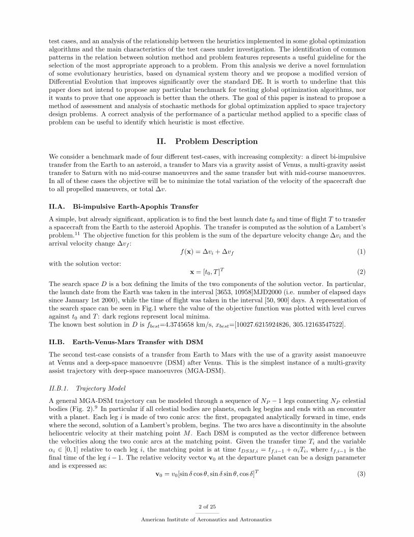
The results of the tests are summarized in Tables 1 and 2, where success probability (Table 1) and bestvalue, mean and variance of best results (Table 2) are given for each of the 20 settings of the five stochasticsolvers.For both EA and EVM cases, success probability allows a fair classification and gives a clear indication ofthe best performing algorithms. If we look only at the set of evolutionary based algorithms (DE, GA andPSO), algorithms DE10e and DE20e perform undoubtedly better than the others and algorithms GA100/200-GA200/400-GA400/600 appear to be the worst performing ones. Algorithm DE5e wins a bronze medal, butif we can be confident in its third position for the EVM problem, we cannot have the same level of confidenceregarding the third position for EA, because of the proximity of other algorithms. Actually, due to thebinomial nature of the success and the adopted sample size, it is not possible to discriminate fairly betweenalgorithms for which the success distance is smaller than the expected error (0.05 in our computations).Therefore, algorithm DE10e has to be considered at the same level as algorithms PSO1007, PSO509, forexample, and other PSO settings. For the same reasons, we can say that, among the PSO settings, algorithmsPSO1007 and PSO509 perform better than algorithm PSO1005 but the remaining PSO algorithms work atthe same level.An analogous vagueness is displayed by most of the evolutionary based algorithms when applied to EVMand almost all of them when applied to EVVEJS and EVVEJSdsm. On the other hand, MS and MBHshows remarkable performance in all the test cases with the simple MS winning over all the others in the EAcase. For the EVVEJS case, all the algorithms but MBH appear practically unsuccessful, because, even ifthe success probability cannot be considered really 0 due to the error margin, it is ≤ 0.12, according to theexpected error. MBH is the only algorithm that can be practically used to solve this problem with a success≤ 0.34. For EVVEJSdsm case even MBH is performing poorly, with a success ≤ 0.08.For cases where the success probability cannot give practically useful information to classify the algorithms,the user could be tempted to use the values of mean and variance, but this practice is strongly heedless.Even if we suppose mean and variance are correct (in some way), looking at these two values can bring toincorrect conclusions. For instance, if we consider the values for the algorithms PSO1009 and GA400 appliedto EVM, we could conclude that algorithm GA400 performs better than algorithm PSO1009, because of asmaller mean value and a smaller variance (regarded as an index of robustness). But, if we are interested in

13 of 25


Table 1. Success for the 20 algorithms on the four test-cases. To compute the success, following tolf values were used:0.001 for EA, 3 − fbest for EVM, 5 − fbest for EVVEJS and 8.5 − fbest for EVVEJSdsm

DE5c DE10c DE20c DE5e DE10e DE20e PSO505 PSO1005 PSO2005 PSO507

EA 0.140 0.300 0.355 0.450 0.770 0.855 0.355 0.345 0.410 0.395

EVM 0.050 0.050 0.050 0.150 0.250 0.370 0.040 0.035 0.080 0.045

EVVEJS 0.020 0.005 0.015 0.000 0.000 0.000 0.000 0.005 0.000 0.000

EVVEJSdsm 0.01 0.000 0.000 0.000 0.000 0.000 0.000 0.000 0.000 0.000

PSO1007 PSO2007 PSO509 PSO1009 PSO2009 GA100/200 GA200/400 GA400/600 MS MBH

EA 0.425 0.410 0.435 0.385 0.420 0.160 0.240 0.105 0.93 0.82

EVM 0.060 0.055 0.035 0.070 0.075 0.005 0.010 0.035 0.625 0.765

EVVEJS 0.000 0.000 0.000 0.000 0.000 0.000 0.000 0.005 0.07 0.29

EVVEJSdsm 0.000 0.000 0.000 0.000 0.000 0.000 0.000 0.000 0.000 0.030

global optimal solutions, algorithm PSO1009 is noticeably better: it is able to find the global solution, evenif it is less robust and gets stuck many times in a far basin (see Figs. 5 and 7).In order to solve an uncertainty condition, for instance when the success probability appears uniformlynull, relaxing the tolf value could be useful. Focusing on the EVVEJS case, there is no way to correctlydiscriminate among the algorithms on the basis of data in Table 1, but if the success threshold is raised from5 to 5.3, then a superior performance of GAs is revealed. Most likely, this behavior is due to a combination ofdifferent features, such as larger population, the mutation search operator and a non-deterministic selectionoperator, which in this complex case reduces the speed of local convergence, preserves diversity and allowsfor a better exploration of the search space.For the EVVEJSdsm case we are not so “lucky”. Raising the success threshold from 8.5 to 9 (see Table3) identifies MBH as the only one algorithm practically able to handle this problem, but does not give anyuseful information to discriminate among the other algorithms. Only the DEc series and MS are able tofind solutions with an objective value below 9, but the success rate is so low and similar that discriminatingbetween the two would be difficult.

2 4 6 80

0.5

1

1.5

2

2.5

fbest

pdf

MPGA EVM 20000 feval

discreteparzengaussian

2 3 4 5 60

1

2

3

4

fbest

pdf

.MPGA EVM 40000 feval


2 3 4 5 60

1

2

3

4

fbest

pdf

MPGA EVM 60000 feval


2 3 4 5 60

1

2

3

4

5

fbest

pdf

.MPGA EVM 100000 feval


Figure 7. Pdfs, for the EVM case with the GA algorithm.

In Figs. 8 to 11 we present two interesting cases. Figs. 8 and 9 represent the pdf and the success rate for theMBH algorithm with ρ = 0.1 applied to the EVVEJS case with no deep space manoeuvres while Figs. 10 and11 represent the pdf and the success rate of the DE5c algorithm applied to the same case. MBH distributesthe solutions over a few distant minima for a low number of function evaluations but then quickly converges

14 of 25


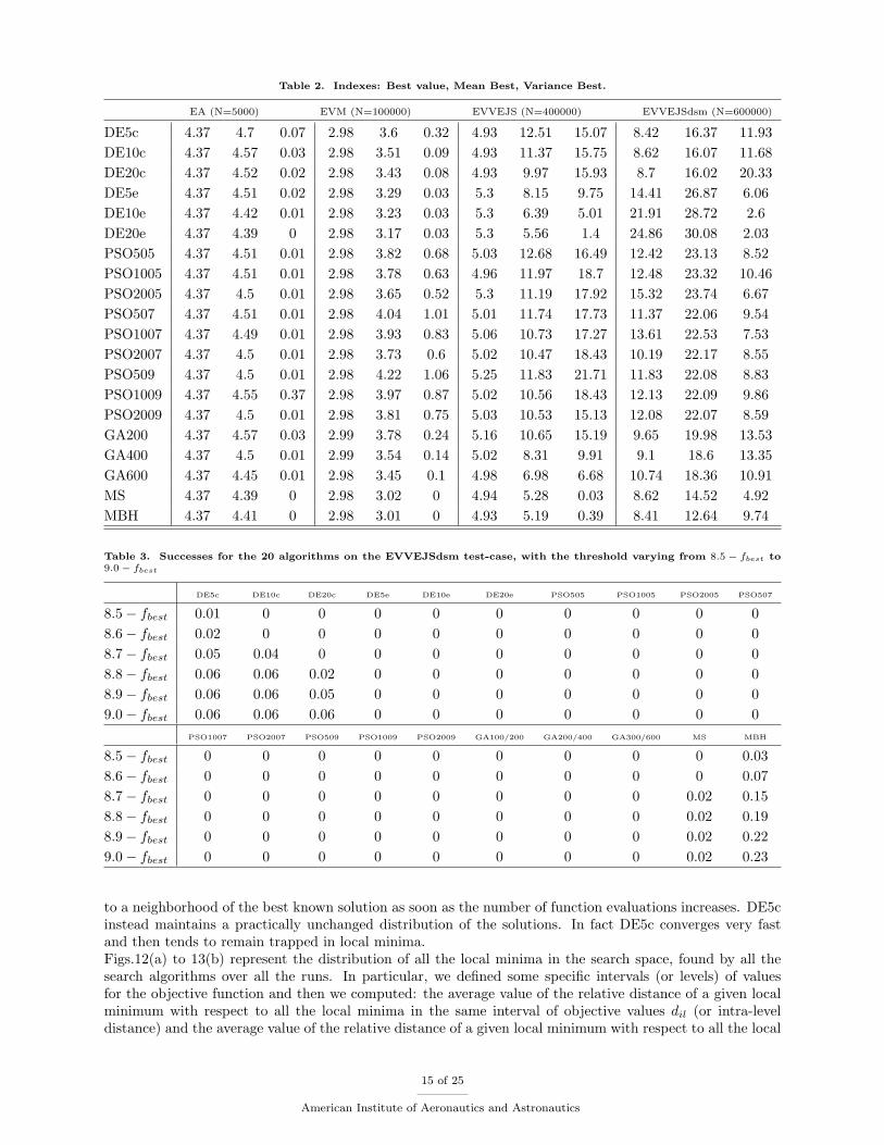
Table 2. Indexes: Best value, Mean Best, Variance Best.

EA (N=5000) EVM (N=100000) EVVEJS (N=400000) EVVEJSdsm (N=600000)

DE5c 4.37 4.7 0.07 2.98 3.6 0.32 4.93 12.51 15.07 8.42 16.37 11.93

DE10c 4.37 4.57 0.03 2.98 3.51 0.09 4.93 11.37 15.75 8.62 16.07 11.68

DE20c 4.37 4.52 0.02 2.98 3.43 0.08 4.93 9.97 15.93 8.7 16.02 20.33

DE5e 4.37 4.51 0.02 2.98 3.29 0.03 5.3 8.15 9.75 14.41 26.87 6.06

DE10e 4.37 4.42 0.01 2.98 3.23 0.03 5.3 6.39 5.01 21.91 28.72 2.6

DE20e 4.37 4.39 0 2.98 3.17 0.03 5.3 5.56 1.4 24.86 30.08 2.03

PSO505 4.37 4.51 0.01 2.98 3.82 0.68 5.03 12.68 16.49 12.42 23.13 8.52

PSO1005 4.37 4.51 0.01 2.98 3.78 0.63 4.96 11.97 18.7 12.48 23.32 10.46

PSO2005 4.37 4.5 0.01 2.98 3.65 0.52 5.3 11.19 17.92 15.32 23.74 6.67

PSO507 4.37 4.51 0.01 2.98 4.04 1.01 5.01 11.74 17.73 11.37 22.06 9.54

PSO1007 4.37 4.49 0.01 2.98 3.93 0.83 5.06 10.73 17.27 13.61 22.53 7.53

PSO2007 4.37 4.5 0.01 2.98 3.73 0.6 5.02 10.47 18.43 10.19 22.17 8.55

PSO509 4.37 4.5 0.01 2.98 4.22 1.06 5.25 11.83 21.71 11.83 22.08 8.83

PSO1009 4.37 4.55 0.37 2.98 3.97 0.87 5.02 10.56 18.43 12.13 22.09 9.86

PSO2009 4.37 4.5 0.01 2.98 3.81 0.75 5.03 10.53 15.13 12.08 22.07 8.59

GA200 4.37 4.57 0.03 2.99 3.78 0.24 5.16 10.65 15.19 9.65 19.98 13.53

GA400 4.37 4.5 0.01 2.99 3.54 0.14 5.02 8.31 9.91 9.1 18.6 13.35

GA600 4.37 4.45 0.01 2.98 3.45 0.1 4.98 6.98 6.68 10.74 18.36 10.91

MS 4.37 4.39 0 2.98 3.02 0 4.94 5.28 0.03 8.62 14.52 4.92

MBH 4.37 4.41 0 2.98 3.01 0 4.93 5.19 0.39 8.41 12.64 9.74

Table 3. Successes for the 20 algorithms on the EVVEJSdsm test-case, with the threshold varying from 8.5 − fbest to9.0 − fbest

DE5c DE10c DE20c DE5e DE10e DE20e PSO505 PSO1005 PSO2005 PSO507

8.5− fbest 0.01 0 0 0 0 0 0 0 0 0

8.6− fbest 0.02 0 0 0 0 0 0 0 0 0

8.7− fbest 0.05 0.04 0 0 0 0 0 0 0 0

8.8− fbest 0.06 0.06 0.02 0 0 0 0 0 0 0

8.9− fbest 0.06 0.06 0.05 0 0 0 0 0 0 0

9.0− fbest 0.06 0.06 0.06 0 0 0 0 0 0 0

PSO1007 PSO2007 PSO509 PSO1009 PSO2009 GA100/200 GA200/400 GA300/600 MS MBH

8.5− fbest 0 0 0 0 0 0 0 0 0 0.03

8.6− fbest 0 0 0 0 0 0 0 0 0 0.07

8.7− fbest 0 0 0 0 0 0 0 0 0.02 0.15

8.8− fbest 0 0 0 0 0 0 0 0 0.02 0.19

8.9− fbest 0 0 0 0 0 0 0 0 0.02 0.22

9.0− fbest 0 0 0 0 0 0 0 0 0.02 0.23

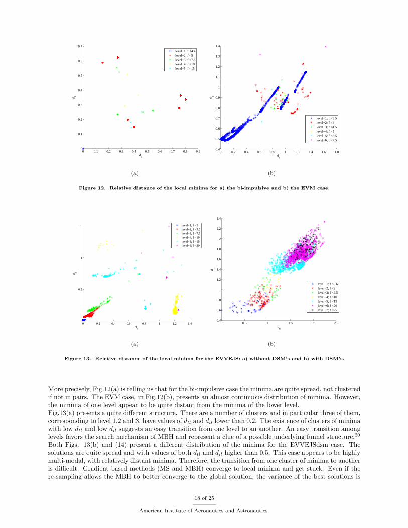
to a neighborhood of the best known solution as soon as the number of function evaluations increases. DE5cinstead maintains a practically unchanged distribution of the solutions. In fact DE5c converges very fastand then tends to remain trapped in local minima.Figs.12(a) to 13(b) represent the distribution of all the local minima in the search space, found by all thesearch algorithms over all the runs. In particular, we defined some specific intervals (or levels) of valuesfor the objective function and then we computed: the average value of the relative distance of a given localminimum with respect to all the local minima in the same interval of objective values dil (or intra-leveldistance) and the average value of the relative distance of a given local minimum with respect to all the local

15 of 25


−10 0 10 20 300

0.2

0.4

0.6

0.8

1

fbest

pdf

MBH EVVEJS 100000 feval


0 5 10 150

0.5

1

1.5

2

fbest

pdf



0 5 10 150

0.5

1

1.5

2

fbest

pdf



0 5 10 150

0.5

1

1.5

2

2.5

fbest

pdf



Figure 8. Pdf for the MBH applied to the solution of the EVVEJS case with no DSMs.

0 50 100 150 2000

0.2

0.4

0.6

0.8

1

Number of runs

Succ

ess

Rat

e

100000 feval

0 50 100 150 2000

0.2

0.4

0.6

0.8

1

Number of runs

Succ

ess

Rat

e

200000 feval

0 50 100 150 2000

0.2

0.4

0.6

0.8

1

Number of runs

Succ

ess

Rat

e

300000 feval

df1.1df1.2df1.3df1.4df1.5df1.6df

0 50 100 150 2000

0.2

0.4

0.6

0.8

1

Number of runs

Succ

ess

Rat

e

400000 feval

Figure 9. Success rate of the MBH applied to the solution of the EVVEJS case with no DSMs.

minima in the interval with lower values of the objective function dtl (or trans-level distance). The figuresgive an immediate representation of the diversity of the local minima in the search space (different colorscorrespond to different levels). Note that the two quantities dil and dtl can be related to the Shannon’sdiversity index.23 In fact, if both dtl and dil are large then the solutions belonging to each species (theintervals of f) are well spread and distant from the solutions of the lower level. In this case, if we considered

16 of 25


−20 0 20 400

0.1

0.2

0.3

0.4

fbest

pdf

DE EVVEJS 100000 feval


−20 0 20 400

0.1

0.2

0.3

0.4

fbest

pdf



−20 0 20 400

0.1

0.2

0.3

0.4

fbest

pdf



−20 0 20 400

0.1

0.2

0.3

0.4

fbest

pdf



Figure 10. Pdf for the DE applied to the solution of the EVVEJS case with no DSMs.

0 50 100 150 2000

0.2

0.4

0.6

0.8

1

Number of runs

Succ

ess

Rat

e



0 50 100 150 2000

0.2

0.4

0.6

0.8

1

Number of runs

Succ

ess

Rat

e



0 50 100 150 2000

0.2

0.4

0.6

0.8

1

Number of runs

Succ

ess

Rat

e



0 50 100 150 2000

0.2

0.4

0.6

0.8

1

Number of runs

Succ

ess

Rat

e



Figure 11. Success rate of the DE applied to the solution of the EVVEJS case with no DSMs.

each solution as a separate species the the value of the diversity index would be high. If both dtl and dilare small the solutions are clustered and close to each other, therefore species are made of large groups ofsolutions and the diversity index would be low. The index would be low also for dil small and dtl large andwould be large for dil large and dtl small. It should be noted that dtl and dil give a better representationof the actual diversity because they consider also the reciprocal distance in the solution space while theShannon’s index is generally associated only to the separation in the criteria space.26

17 of 25


0 0.1 0.2 0.3 0.4 0.5 0.6 0.7 0.8 0.90

0.1

0.2

0.3

0.4

0.5

0.6

0.7

dtl

d il

level−1; f <4.4level−2; f <5level−3; f <7.5level−4; f <10level−5; f <15

(a)

0 0.2 0.4 0.6 0.8 1 1.2 1.4 1.6 1.80.4

0.5

0.6

0.7

0.8

0.9

1

1.1

1.2

1.3

1.4

dtl

d il

level−1; f <3.5level−2; f <4level−3; f <4.5level−4; f <5level−5; f <5.5level−6; f <7.5

(b)

Figure 12. Relative distance of the local minima for a) the bi-impulsive and b) the EVM case.

0 0.2 0.4 0.6 0.8 1 1.2 1.40

0.5

1

1.5

dtl

d il

level−1; f <5level−2; f <5.5level−3; f <7.5level−4; f <10level−5; f <15level−6; f <20

(a)

0 0.5 1 1.5 2 2.50.4

0.6

0.8

1

1.2

1.4

1.6

1.8

2

2.2

2.4

dtl

d il

level−1; f <8.6level−2; f <9level−3; f <9.5level−4; f <10level−5; f <15level−6; f <20level−7; f <25

(b)

Figure 13. Relative distance of the local minima for the EVVEJS: a) without DSM’s and b) with DSM’s.

More precisely, Fig.12(a) is telling us that for the bi-impulsive case the minima are quite spread, not clusteredif not in pairs. The EVM case, in Fig.12(b), presents an almost continuous distribution of minima. However,the minima of one level appear to be quite distant from the minima of the lower level.Fig.13(a) presents a quite different structure. There are a number of clusters and in particular three of them,corresponding to level 1,2 and 3, have values of dtl and dil lower than 0.2. The existence of clusters of minimawith low dtl and low dil suggests an easy transition from one level to an another. An easy transition amonglevels favors the search mechanism of MBH and represent a clue of a possible underlying funnel structure.20

Both Figs. 13(b) and (14) present a different distribution of the minima for the EVVEJSdsm case. Thesolutions are quite spread and with values of both dtl and dil higher than 0.5. This case appears to be highlymulti-modal, with relatively distant minima. Therefore, the transition from one cluster of minima to anotheris difficult. Gradient based methods (MS and MBH) converge to local minima and get stuck. Even if there-sampling allows the MBH to better converge to the global solution, the variance of the best solutions is

18 of 25


0 10 20 30 400

0.05

0.1

0.15

0.2

fbest

pdf

MBH EVVEJS−DSM 150000 feval


0 10 20 300

0.05

0.1

0.15

0.2

0.25

fbest

pdf



0 10 20 300

0.05

0.1

0.15

0.2

0.25

fbest

pdf



0 10 20 300

0.1

0.2

0.3

0.4

fbest

pdf



Figure 14. Examples of pdfs, for the EVVEJS case with DSM and the MBH optimizer.

still very high. Note that in the case of the EVVEJS problem with no deep-space manoeuvre running theMBH with no re-sampling provides an increase in performance from 29% to 37.5%.Note that although the dtl − dil plots can provide clues on the characteristics of the search space, itsstructure can be revealed only by an analysis of the actual position of all the local optima and not just bya measurement of their reciprocal distance. On the other hand, knowing all the local optima of a problemwould mean having solved completely the problem. Therefore, the dtl−dil plane can be useful either to inferfrom the characteristics of a benchmark test case the characteristics of other unsolved problems belongingto the same class (i.e. with an expected similar structure) or to devise the proper heuristics for solving anew problem when some local optima are already available.

V. A Dynamical System Prospective

In this section we look at some evolutionary heuristics from a different prospective in the attempt to betterunderstand the dynamics of the search process regardless of the problem under investigation. This analysiswill be used to improve the performance of one of the algorithms tested above. In particular, we note thatboth DE and PSO can be rewritten in a compact form as a discrete dynamical system:

vi,k+1 = (1− c)vi,k + ui,k

xi,k+1 = xi,k + νS(xi,k + vi,k+1)vi,k+1

(22)

withν = min([vmax, vi,k+1])/vi,k+1 (23)

The control ui,k defines the next point that will be sampled for each one of the existing points in the solutionspace, the vectors xi,k and vi,k define the current state of a point in the solution space at stage k of thesearch process and c is a viscosity, or dissipative coefficient, for the process. Eq. (23) represents a limitsphere around the point xi,k at stage k of the search process.In addition to Eq. (22) and Eq. (23), each optimization algorithm has heuristics responsible for selectingthe new candidate points generated with ui,k. The selection operator is expressed through the functionS(xi,k + vi,k+1) which can be either 1 if the candidate point is accepted or 0 if it is not accepted.Differential Evolution, in its basic form, has the ui,k defined by Eq.(13), viscosity c = 1 and vmax = +∞.The selection function S can be either 1 or 0 depending on the relative value of the objective functionof the new candidate individual generated with Eq.(13) with respect to the one of the current individual(see Algorithm 2). Particle swarm optimization has ui,k defined in Eq.(16) with the viscosity term c =1 − [0.4 + 0.8(kmax − k)/(kmax − 1)], no mask and no selection, therefore S is always equal to 1 but v is

19 of 25


constrained by Eq. (23). Note that if we take c2r2 = Fe, c1r1 = e and replacing xgi,k with one of theindividuals in the population, then PSO translates into DE and vice versa, we can go from DE to PSO justby properly defining the selection of the individuals xi1,k,xi2,k,xi3,k, the value of the coefficients c, c1, c2, νand the selection function S.The discrete dynamical system in Eqs. (22) can be rewritten in matrix form as follows:[

xi,k+1

vi,k+1

]= Ji,k

{xi,k

vi,k

}(24)

and if we consider all the individuals in the population:[ xk+1

vk+1

]= Jk

{ xk

vk

}(25)

The map (25) allows for a number of considerations on the evolution of the search process and therefore onthe properties of the global optimization algorithm. In particular the map can:

• Diverge to infinity. In this case the discrete dynamical system is unstable, the global optimizationalgorithm is not convergent.

• Converge to a fixed point in D. In this case the global optimization algorithm is simply convergent inD and we can define a stopping criterion. Once the search is stopped we can define a restart procedure.Depending on the convergence profile, the use of a restart procedure can be more or less efficient.

• Converge to a limit cycle in which the same points in D are re-sampled periodically. Even in this casewe can define a stopping criterion and a restart procedure.

• Converge to a strange (chaotic) attractor. In this case a stopping criterion cannot be clearly definedbecause different points are sampled at different iterations.

We have seen in the previous sections that the heuristics implemented in MBH are particularly effective.MBH is based on a Newton (or quasi-Newton) method for local minimization and on a restart of the searchwithin a neighborhood Nρ of a local minimum. We can view such local optimization methods as dynamicalsystems where the evolution of the systems at each iteration is controlled by some map Jk. Under suitableassumptions, the systems converge to a fixed point. For instance, if f is convex and C2 in a small enoughdomain Dk containing a local minimum which satisfies some regularity conditions, Newton’s map convergesquadratically to a single fixed point (the local minimum) in Dk.The motivations for using different dynamical systems are: dropping the requirement for the continuity anddifferentiability of f ; automatically reducing the size of the region in which a candidate point is generated(the basic version of MBH has a constant size of Nρ); and performing not only a local exploration of theneighborhood, but also a global one. For instance, in the specific case of simple Differential Evolution, c = 1and ν = 1, therefore we have the reduced map:

xi,k+1 = xi,k + S(xi,k + ui,k)ui,k (26)

or in matrix form for the entire population xk+1 = Jkxk. The interest is now in the properties of map (26).We start by observing that if S(xk + uk) = 1⇔ f(xk + uk) < f(xk) the global minimizer xg ∈ D is a fixedpoint for (26) since every point x ∈ D is such that f(x) > f(xg).Then, let us assume that at every iteration k we can find two connected subsets Dk and D∗

k of D such thatf(xk) < f(x∗

k), ∀xk ∈ Dk,∀x∗k ∈ D∗

k \Dk, and let us also assume that Pk ⊆ Dk while Pk+1 ⊆ D∗k (recall that

Pk and Pk+1 denote the populations at iteration k and k+1 respectively). If xl is the lowest local minimumin Dk, then xl is a fixed point in Dk for (26). In fact, every point generated by (26) (or (25)) must be in Dk

and f(xl) < f(x), ∀x ∈ Dk

Now we want to know if there are other fixed points for the dynamics (26) and if we can always have a simpleconvergence in Dk. First of all we note that if for every k, Pk ⊆ Dk and Pk+1 ⊆ D∗

k, then the reciprocaldistance of the individuals cannot grow indefinitely because of the map (26), therefore the map cannot bedivergent.Then, if we assume that the function f is strictly quasi-convex25 in Dk, we can prove that (26) converges toa fixed point in Dk. We first need the following lemma.

20 of 25


Lemma V.1 If f is continuous and strictly quasi-convex on a compact set Dj, the following minimizationproblem with F ∈ (0, 1) has a strictly positive minimum value δr(ϵ):

δr(ϵ) = min g(y1,y2) = f(y2)− f(Fy1 + (1− F )y2)

s.t. y1,y2 ∈ Dk

∥y1 − y2∥ ≥ ϵ

f(y1) ≤ f(y2)

(27)

Proof Since f is strictly quasi-convex g(y1, y2) > 0, ∀y1, y2 ∈ D; furthermore, the feasible region iscompact and, therefore, according to Weierstrass’ theorem the function g attains its minimum value overthe feasible region. If we denote by (y∗

1,y∗2) a global minimum point of the problem, then we have

δr(ϵ) = g(y∗1,y

∗2) > 0. (28)

Theorem V.2 Given a function f that is strictly quasi-convex over Dk and a population Pk ∈ Dk, then ifF ∈ (0, 1) and S(xk + uk) = 1 ⇔ f(xk + uk) < f(xk) , the population Pk converges to a fixed point in Dk

for k →∞.

Proof We propose two distinct proofs for this result. The first one is simpler but requires an additionalassumption. The second one is more complicated but also more general.

The first simpler proof requires the additional assumption that the population always has an individualxj,k that is strictly better than the others, i.e. f(xj,k) < f(xi,k) for any i = j, then the map (26) at eachiteration k can generate, with strictly positive probability, a displacement (xj,k − xi,k) for all the membersof the population. This means that at each iteration we have a strictly positive probability that the wholepopulation collapses into a single point. Then, for k → ∞ the whole population collapses to a single pointwith probability one.

The more complicated and more general proof is the following. By contradiction let us assume that wedo not have convergence to a fixed point. Then, it must hold that:

infkmax{∥xi,k − xj,k∥, i, j ∈ [1, ..., npop]} ≥ ϵ > 0 (29)

At every generation k the map can generate with a strictly positive probability, a displacement F (xi∗,k −xj∗,k), where i

∗ and j∗ identify the individuals with the maximal reciprocal distance, such that the candidatepoint is xcand = Fxi∗,k+(1−F )xj∗,k with f(xi∗,k) ≤ f(xj∗,k). Since the function f is strictly quasi-convex,the candidate point is certainly better than xj∗,k and, therefore, is accepted by S. Now, in view of (29) andof Lemma (V.1) we must have that

f(xcand) ≤ f(xj,k)− δr(ϵ). (30)

Such reduction will occur with probability one infinitely often, and consequently the function value of atleast one individual will be, with probability one, infinitely often reduced by δr(ϵ). But this way the valueof the objective function of such individual would diverge to −∞, which is a contradiction because f isbounded from below over the compact set Dk.

In particular, the above result shows that, when the population of DE lies at each iteration in the neigh-borhood of a local minimum satisfying some regularity assumption (e.g., the Hessian at the local minimumis definite positive, implying strict convexity in the neighborhood), then DE will certainly converge to afixed point. For general functions, we can not always guarantee that the population will converge to a fixedpoint, but we can show that the maximum difference between the objective function values in the populationconverges to 0, i.e. the points in the population tend to belong to the same level set.

Theorem V.3 Given a function f and a population Pk ∈ Dk, then if F ∈ (0, 1) and S(xk + uk) = 1 ⇔f(xk + uk) < f(xk) , the following holds

maxi,j∈[1,...,npop]

| f(xj,k)− f(xi,k) |→ 0,

as k →∞.

21 of 25


Proof Let S∗k denote the set of best points in population Pk, i.e.

S∗k = {xj,k : f(xj,k) ≤ f(xi,k) ∀ i ∈ [1, . . . , npop]}

At each iteration k there is a strictly positive probability that the whole population will be reduced to S∗k at

the next iteration. In other words, there is a strictly positive probability for the event that the populationat a given iteration will be made up by points all with the same objective function value. Therefore, suchevent will occur infinitely often with probability one. Let us denote with {kh}h=1,... the infinite subsequenceof iterations at which the event is true, and let

∆h = f(xi,kh)− f(xi,kh+1

)

be the difference of the objective function values at two consecutive iterations kh and kh+1 (note that, sinceat iterations kh, h = 1, . . . the objective function values are all equal and any i can be employed in the abovedefinition). It holds that for all i, j ∈ [1, . . . , npop]

| f(xj,k)− f(xi,k) |≤ ∆h ∀ k ∈ [kh, kh+1].

Therefore, if we are able to prove that ∆h → 0, as h→∞, then we can also prove the result of our theorem.Let us assume by contradiction that ∆h → 0. Then, there will exist a δ > 0 such that ∆h ≥ δ infinitelymany times. But this would lead to function values diverging to −∞ and, consequently, to a contradiction.

As a consequence of these results, a possible stopping criterion for DE would be to stop when the differencebetween the function values in the population drops below a given threshold. However, this could causepremature convergence. Indeed, even if at some iteration the value ∆h drops to 0, this does not necessarilymean that the algorithm will be unable to make further progress. Therefore, since the most likely situation isthe convergence to a single point, we can alternatively use as a stopping criterion the fact that the maximumdistance between points in the population drops below a threshold.

5 10 15 20 25 30 35

0

0.1

0.2

0.3

0.4

0.5

0.6

0.7

0.8

Iterations

max distancemin distance

(a)

5 10 15 20 25 30 350

0.2

0.4

0.6

0.8

1

1.2

1.4

1.6

Iterations

Eig

enva

lue

(b)

Figure 15. Dissipative properties of Differential Evolution:a) max and min distance of the individuals in the populationfrom the origin, b) eigenvalues with the number of evolutionary iterations.

To further verify the contraction property of the dynamics in Eq. (26) we can look at the eigenvalues of thematrix Jk.If the population cannot diverge the eigenvalues cannot have norm always > 1. Furthermore, according toTheorem V.2 if the function f is strictly quasi-convex in Dk the population converges to a fixed point in Dk,which implies that the map (26) is a contraction in Dk and therefore the eigenvalues should have norm onaverage lower than 1. This can be illustrated with the following test. Consider a population of 8 individualsand a Dk enclosing the minimum of a paraboloid with the minimum at the origin. We compute, for eachstep k, the distance of the closest and farthest individual from the local minimum and the eigenvalues of thematrix J. Fig.15 shows the behavior of the eigenvalues and of the distance from the origin. From the figure

22 of 25


Algorithm 8 Inflationary Differential Evolution Algorithm (IDEA)

1: Set values for npop, CR and F , set nfeval = 0 and k = 1, set threshold tolconv2: Initialize xi,k and vi,k for all i ∈ [1, ..., npop]3: Create the vector of random values r ∈ U [0, 1] and the mask e = r < CR

4: for all i ∈ [1, ..., npop] do5: Select three individuals xi1 ,xi2 ,xi3

6: Create the vector ui,k = e[(xi3,k − xi,k) + F (xi2,k − xi1,k)]7: vi,k+1 = (1− c)vi,k + ui,k

8: Compute S and ν9: xi,k+1 = xi,k + Sνvi,k+1

10: nfeval = nfeval + 111: end for12: k = k + 113: ρA = max(∥xi,k − xj,k∥) for ∀xi,k,xj,k ∈ Psub ⊆ Pk

14: if ρA < tolconv then15: Define a bubble Dl such that xi,k ∈ Dl for ∀xi,k ∈ Psub and Psub ⊆ Pk

16: Ag = Ag + {xbest} where xbest = argmini f(xi,k)17: Initialize xi,k and vi,k for all i ∈ [1, ..., npop], in the bubble Dl ⊆ D18: end if19: Termination Unless nfeval ≥ nfevalmax, goto Step 3

we can see that for all iterations, the value of the norm of all the eigenvalues is in the interval [0, 1] exceptfor one eigenvalue at iteration 12. However, since on average the eigenvalue is lower than 1, the populationcontracts as represented in Fig.15a.

0 5 10 150

1

2

3

fbest

pdf

IDEA 100000 feval


0 5 10 150

1

2

3

4

fbest

pdf

IDEA 200000 feval


0 5 10 150

1

2

3

fbest

pdf

IDEA 300000 feval


0 5 10 150

1

2

3

fbest

pdf

IDEA 400000 feval


Figure 16. Pdf for IDEA applied to the solution of the EVVEJS case with no DSMs.

If multiple minima are contained in Dk then it can be experimentally verified that the population contractsto a number of clusters initially converging to a number of local minima and eventually to the lowest amongall of the identified local minima. Now, if a cluster contracts we can define a bubble Dl ⊆ D, containing thecluster, and re-initialize a subpopulation Psub in Dl when the maximum distance ρA = max(∥xi−xj∥) among

23 of 25


0 50 100 150 2000

0.2

0.4

0.6

0.8

1

Number of runsSu

cces

s R

ate

IDEA 100000 feval


0 50 100 150 2000

0.2

0.4

0.6

0.8

1

Number of runs

Suc

cess

Rat

e

IDEA 200000 feval


0 50 100 150 2000

0.2

0.4

0.6

0.8

1

Number of runs

Succ

ess

Rat

e

IDEA 300000 feval

0 50 100 150 2000

0.2

0.4

0.6

0.8

1

Number of runs

Suc

cess

Rat

e

IDEA 400000 feval


Figure 17. Success rate of IDEA applied to the solution of the EVVEJS case with no DSMs.

the elements in the cluster collapses below a value tolconv. Every time a subpopulation is re-initialized thebest solution xbest of the cluster is saved in an archive Ag. This process leads to the modified DE algorithm8. Note that the contraction of the population given, for example, by the metric ρA, is a stopping criterionthat does not depend explicitly on the value of the objective function but on the contractive properties ofthe map in Eq.(26).The new algorithm was tested again on the EVVEJS case without DSM. For the tests presented in this paperwe did not try to identify the formation of clusters made of subsets of the population. Instead, we restartedthe whole population, inside a single bubble, when the maximum distance among its individuals was belowtolconv. The result is represented in Figs. 16 and 17. With respect to the original version of DE (see Fig.11) the improvement in the success rate is remarkable and reaches almost 40%. Unlike the MBH version inFig. 8, for IDEA we did not operate a re-sampling over the entire D when no improvement was registered.This could be the reason for the lower success rate when the tolerance tolf is increased. On the other hand,we should remark that IDEA manages to converge to the best known solution, while MBH remains slightlyabove that value (both with and without re-sampling). This is due to the fact that in a small neighborhoodof the best known solution there is a large number of local minima, all with similar values but irregularlydistributed. In this case the ability of the DE map to automatically adapt the size of the region in which itgenerates the candidate points, represents an advantage over the fixed neighborhood Nρ of MBH.

VI. Conclusion

In this paper we presented an approach to test global optimization algorithms applied to the solution ofspace trajectory design problems. We discussed the relevance of some performance indexes, in particularmean, variance, best value and success rate. The last one offers a better and more precise estimationof the actual performance of an algorithm when applied to a standard benchmark. The selection of thetest cases in the benchmark is quite important since the characteristics of the problem, and therefore theperformance of a given algorithm, can change significantly even by changing the modeling of the sameproblem, as demonstrated by the two models for the same EVVEJS transfer. The use of the success rateoffers a distinctive advantage of a precise a priori definition of the required number of runs to correctlyestimate the success rate. The use of mean and variance, instead, showed to be misleading in some casesand inconclusive in others since the distribution of the results was demonstrated to be non-Gaussian.Finally we presented a dynamical system interpretation of some evolutionary heuristics. By analyzing some

24 of 25


dynamical properties of differential evolution in relation to the characteristics of the problems in the bench-mark, we derived a new algorithm that outperformed the standard DE and all the tested EA, becomingcompetitive against the best performing tested stochastic method, the MBH.An interesting result of the analysis presented in this paper is that even a single specific heuristic cansignificantly improve the performance of a search method applied to a particular class of problems. Onthe other hand, this fact highlights the importance of a proper coupling between heuristics and problemstructure which is not always possible a priori.

References

1P.J. Gage, R.D. Braun, I.M. Kroo, Interplanetary trajectory optimization using a genetic algorithm, Journal of the Astro-nautical Sciences, 43 (1) (1995) 59-75.2G. Rauwolf, V. Coverstone-Carroll, Near-optimal low-thrust orbit transfers generated by a genetic algorithm, Journal of

Spacecraft and Rockets, 33 (6) (1996) 859-862.3Kim, Y.H., and Spencer, D.B., ”Optimal Spacecraft Rendezvous Using Genetic Algorithms”, Journal of Spacecraft and

Rockets, Vol. 39, No. 6, Nov.-Dec. 2002, pp. 859-865.4Abdelkhalik O., Mortari D., ”N-Impulse Orbit Transfer Using Genetic Algorithms”, Journal of Spacecraft and Rockets, Vol.

44, No. 2, March-April 2007, pp. 456-459.5Olds A. D., Kluever C. A., Cupples M.L. ”Interplanetary Mission Design Using Differential Evolution”, Journal of Spacecraft

and Rockets, Vol. 44, No. 5, Sept.-Oct. 2007, pp. 1060-1070.6Di Lizia P., Radice G., ”Advanced Global Optimization Tools for Mission Analysis and Design” Final Report of ESA Ariadna

ITT AO4532,Call 03/4101, 2004.7D. R. Myatt, V.M. Becerra, S.J. Nasuto, and J.M. Bishop, ”Advanced Global Optimization Tools for Mission Analysis and

Design,” Final Rept. ESA Ariadna ITT AO4532/18138/04/NL/MV,Call03/4101, 2004.8Vasile M., Summerer L., De Pascale P., Design of Earth-Mars Transfer Trajectories using Evolutionary Branching Techniques,

Acta Astronautica, Vol. 56, pp. 705-720, 2005.9Vasile M., De Pascale P., Preliminary Design of Multiple Gravity-Assist Trajectories, Journal of Spacecraft and Rockets, Vol.

43,No.4, July-August, 2006.10C.J. Adcock. Sample size determination: a review. The Statistician, 46(2):261–283, 1997.11H. Battin. An Introduction to the Mathematics and Methods of Astrodynamics. AIAA, 1999.12M. Clerc. Particle Swarm Optimization. ISTE, 2006.13K.V. Price, R.M. Storn and J.A. Lampinen. Differential Evolution. A Practical Approach to Global Optimization. NaturalComputing Series, Springer, 2005.14A.V. Labunsky, O.V. Papkov, K.G. Sukhanov. Multiple Gravity Assist Interplanetary Trajectories. ESI Book Series, 1998.15M. Mitchell. An introduction to genetic algorithms. MIT Press, 1998.16S.H. Strogatz. Nonlinear Dynamics and Chaos. Westview Press, 2000.17Galor O. Introduction to Stability Analysis of Discrete Dynamical Systems. Macroeconomics, EconPapers, 2004.18C. D. Perttunen and B. E. Stuckman, Lipschitzian Optimization Without the Lipschitz Constant, JOTA, 79(1), (1993)157-181.19Wales D.J, and Doye J. P. K., Global optimization by basin-hopping and the lowest energy structures of Lennard-Jonesclusters containing up to 110 atoms, J. Phys. Chem. A, 101, 5111–5116, (1997).20Leary R. H., Global optimization on funneling landscapes, J. Global Optim., 18, 367–383, (2000).21B.Addis, M. Locatelli, F.Schoen, Local optima smoothing for global optimization, Optimization Methods and Software, 20,417-437 (2005)22M.Locatelli, ”On the multilevel structure of global optimization problems”, Computational Optimization and Applications,30, 5-22 (2005)23Shannon, C.E. A mathematical theory of communication. July and October 1948, Bell System Technical Journal 27: 379-423and 623-65624Vasile I. Istratescu, Fixed Point Theory, An Introduction, D.Reidel, the Netherlands 1981. ISBN 90-277-1224-7 Chapter 7.25Rockafellar, R. T. Convex analysis. 1970, Princeton University Press.26Liu S-H, Mernik M., Bryant B.B. Entropy-Driven Parameter Control for Evolutionary Algorithms. Informatica 31 (2007)4150.27Vasile M., Locatelli M. A Hybrid MultiAgent Approach for Global Trajectory Optimization. Journal of Global Optimization,2008, in press.

25 of 25


Documents

On Testing Global Optimization Algorithms for Space