On the Arctic Boundary Layer

On the Arctic Boundary LayerFrom Turbulence to Climate

Thorsten Mauritsen

Stockholm University

Frontpage image: As a fresh PhD. student I visited Uppsala University January 2003 to attend a seminar byLarry Mahrt. In advance I decided to contact Professor Sergej Zilitinkevich for a discussion after the seminar.Of course, Sergej had forgotten everything about our appointment, so I had to wait around for several hours.Finally, after less than thirty minutes discussion and a piece of paper filled with cryptic notes (the image) thedirections were set for a wonderful collaboration. On the right are the basic assumptions utilized in Paper III.Photo by Malin Mauritsen.

c© Thorsten Mauritsen, Stockholm 2007

ISBN 91-7155-373-8

Printed in Sweden by Universitetsservice US-AB , Stockholm 2007Distributor: Department of Meteorology, Stockholm University

Abstract

The boundary layer is the part of the atmosphere that is in direct contact with the ground viaturbulent motion. At mid-latitudes the boundary layer is usually one or a few kilometers deep,while in the Arctic it is much more shallow, typically a few hundred meters or less. The reason isthat here the absolute temperature increases in the lowest kilometer, making the boundary layersemi-permanently stably stratified. The exchange of heat, momentum and tracers between theatmosphere, ocean and ground under stable stratification is discussed from an observational,modeling and climate-change point of view. A compilation of six observational datasets, or-dered by the Richardson number (rather than the widely used Monin-Obukhov length) revealsnew information about turbulence in the very stably stratified regime. An essentially new tur-bulence closure model, based on the total turbulent energy concept and these observationaldatasets, is developed and tested against large-eddy simulations with promising results. Therole of mesoscale motion in the exchange between the atmosphere and surface is investigatedboth for observations and in idealized model simulations. Finally, it is found that the stablystratified boundary layer is more sensitive to external surface forcing than its neutral and con-vective counterparts. It is speculated that this could be part of the explanation for the observedArctic amplification of climate change.

List of Papers

This thesis is based on the following papers, which are referred to in the textby their Roman numerals:

I Mauritsen, T., G. Svensson and B. Grisogono, 2005: Wave flowsimulations over Arctic leads. Boundary-Layer Meteorology,117(2), 259-273.

II Mauritsen, T. and G. Svensson, 2007: Observations of stablystratified shear-driven atmospheric turbulence at low and highRichardson numbers. Journal of the Atmospheric Sciences,64(2), 645–655.

III Mauritsen, T., G. Svensson, S. S. Zilitinkevich, I. Esau, L. En-ger and B. Grisogono, 2007: A total turbulent energy closuremodel for neutral and stably stratified atmospheric boundary lay-ers. Submitted to Journal of the Atmospheric Sciences.

IV Tjernström, M. and T. Mauritsen, 2007: Mesoscale variability inthe summer Arctic boundary layer. Manuscript.

V Mauritsen, T. and G. Svensson, 2007: Sensitivity of the dry stableboundary layer to external surface forcing. Manuscript.

Reprints were made with kind permission of Springer Science and Business Mediaand the American Meteorological Society. I have been the main contributor and writ-ten most parts of Papers I, II, III and V. The original ideas for Papers I and III belongto Gunilla Svensson and Sergej S. Zilitinkevich, respectively. I had the original ideaof analyzing the micro-barograph data from AOE-2001 for Paper IV, but insufficientfamiliarity with the large observational dataset. Therefore, Michael Tjernström hasdone the major part of the manuscript.

7

Publications not included in the thesis:

• Cuxart J., A. A. M. Holtslag, R. Beare, A. Beljaars, A. Cheng, L.Conangla, M. Ek, F. Freedman, R. Hamdi, A. Kerstein, H. Kita-gawa, G. Lenderik, D. Lewellen. J. Mailhot, T. Mauritsen, V. Perov,G. Schayes, G-J. Steeneveld, G. Svensson, P. Taylor, S. Wunsch, W.Weng and K-M. Xu, 2006. Single-column intercomparison for a sta-bly stratified atmospheric boundary layer. Boundary-Layer Meteorol-ogy, 118, 273–303.

• Mauritsen, T. and E. Källén, 2004. Blocking prediction in an ensem-ble forecasting system. Tellus, 56A, 218-228.

• Steeneveld, G. J., T. Mauritsen, E. I. F. de Bruijn, J. Vila Guerau deArellano, G. Svensson, and A. A. M. Holtslag, 2007. Evaluation ofthe stable boundary layer and diurnal cycle in the limited area mod-els MM5, COAMPS and HIRLAM for three contrasting nights inCASES99. Submitted to Journal of Applied Meteorology and Climate.

8

Contents

1 Introduction . . . . . . . . . . . . . . . . . . . . . . . . . . . . . . . . . . . . . . . . . . 111.1 The Arctic Climate System . . . . . . . . . . . . . . . . . . . . . . . . . . . . . . . . . . . 141.2 Boundary Layers and Turbulence . . . . . . . . . . . . . . . . . . . . . . . . . . . . . . . 171.3 Major Questions Addressed . . . . . . . . . . . . . . . . . . . . . . . . . . . . . . . . . . 20

2 Atmospheric Scales of Motion . . . . . . . . . . . . . . . . . . . . . . . . . . . . . 233 Stably Stratified Boundary Layers . . . . . . . . . . . . . . . . . . . . . . . . . . 29

3.1 Richardson’s Critical Number . . . . . . . . . . . . . . . . . . . . . . . . . . . . . . . . . 313.2 Failure of Obukhovs Length . . . . . . . . . . . . . . . . . . . . . . . . . . . . . . . . . . 34

4 Models of Atmospheric Turbulence . . . . . . . . . . . . . . . . . . . . . . . . . . 374.1 Boundary Layer Models . . . . . . . . . . . . . . . . . . . . . . . . . . . . . . . . . . . . . 424.2 More – Or Less – Diffusion . . . . . . . . . . . . . . . . . . . . . . . . . . . . . . . . . . . 44

5 Climate and Arctic Amplification . . . . . . . . . . . . . . . . . . . . . . . . . . . . 475.1 A Simple Climate Model . . . . . . . . . . . . . . . . . . . . . . . . . . . . . . . . . . . . . 485.2 Arctic Amplification . . . . . . . . . . . . . . . . . . . . . . . . . . . . . . . . . . . . . . . . 50

6 Outlook . . . . . . . . . . . . . . . . . . . . . . . . . . . . . . . . . . . . . . . . . . . . . . 55

1. Introduction

The Earth’s northern polar region is named the Arctic. It is the home of aunique wildlife, including the Polar bear, and highly adapted indigeneouspeoples. It is also one of the least explored and exploited regions on Earthby mankind, due mainly to the immense practical problems with accessingthe region. All of this appears to be changing. The ongoing dramatic climatechanges in the Arctic region has recently received great attention in both thescientific community and in the public media. Alarming reports of sea ice,snow and glaciers melting and thawing tundra, rising sea-levels, reductions ofthe Gulfstream and changes in vegetation and wildlife are flooding the press.Indeed the Arctic region has warmed more than anywhere else on Earth in thepast century; a phenomenon denoted polar amplification. The historic warm-ing rate is roughly twice as fast as the global average.

We have long been fascinated by the Arctic. Through time numerous ex-plorers have attempted to unveil its secrets and many of them have paid withtheir lives. Modern exploration has been conducted since the fifteenth cen-tury, though we believe the Greeks sailed into the North Atlantic, visiting forexample Iceland during their reign. In historical times the explorations wereinitiated by whale hunters. These were soon to be followed by explorers withhigher goals, such as finding a route to the Pacific Ocean and even later themotivation was the pure glory of being the first to reach the North Pole. In1893 the Norwegian explorer and oceanographer Fridtjof Nansen made a se-rious attempt at reaching the pole. He and his crew froze their ship Fram intothe pack ice north of Siberia. Nansen was convinced that the ocean currentswould bring them across the Arctic Ocean towards Svalbard and Greenland.His predictions were correct; Fram drifted across the ocean and reached Nor-way three years later. At some point it became obvious that they would notpass the pole. Determined to reach his goal, Nansen and his companion wentoff on foot, though they were unsuccessful due to the harsh conditions. Theybarely survived on Franz Josefs land and were ultimately rescued by otherexplorers. The first to reach the Pole were the Americans Robert Peary andMatthew Henson. They used the knowledge and skill of the Inuit people ondogsleds, furs, and igloos to achieve their goal. They went from EllesmereIsland to the Pole in just little more than a month in the spring of 1909. To-day scientists and wealthy tourists frequently visit the Central Arctic Oceanaboard modern icebreakers.

11

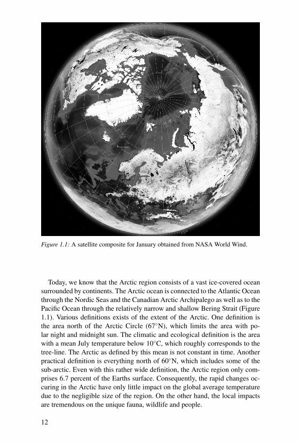
Figure 1.1: A satellite composite for January obtained from NASA World Wind.

Today, we know that the Arctic region consists of a vast ice-covered oceansurrounded by continents. The Arctic ocean is connected to the Atlantic Oceanthrough the Nordic Seas and the Canadian Arctic Archipalego as well as to thePacific Ocean through the relatively narrow and shallow Bering Strait (Figure1.1). Various definitions exists of the extent of the Arctic. One definition isthe area north of the Arctic Circle (67◦N), which limits the area with po-lar night and midnight sun. The climatic and ecological definition is the areawith a mean July temperature below 10◦C, which roughly corresponds to thetree-line. The Arctic as defined by this mean is not constant in time. Anotherpractical definition is everything north of 60◦N, which includes some of thesub-arctic. Even with this rather wide definition, the Arctic region only com-prises 6.7 percent of the Earths surface. Consequently, the rapid changes oc-curing in the Arctic have only little impact on the global average temperaturedue to the negligible size of the region. On the other hand, the local impactsare tremendous on the unique fauna, wildlife and people.

12

Conditions in the Arctic are very different from the rest of the globe. Theenvironment offers challenges to its inhabitants, as well as to scientists try-ing to understand it. There is the sea-ice and tundra on land, clouds appear tobe different, the dark polar night during winter and the midnight sun duringsummer to mention a few. A major theme in the present thesis is the conse-quences of the atmosphere often being more ’layered’ than elsewhere on theglobe. Due to the low temperatures at the surface compared with higher up,air is reluctant to mix vertically, which can result in multiple thin layers ofclouds and pollutants. We refer to the atmosphere as being stably stratified.The lowest kilometer of the Arctic atmosphere is almost permanently stablystratified year around, more so during winter than summer.

Scientists in the 1980’s warned that the Earths climate was warming, aftera period when some researchers claimed that we were heading towards a newice-age. In order to sort things out the Intergovernmental Panel on ClimateChange (IPCC) was jointly established by the World Meteorological Organi-zation (WMO) and the United Nations Environment Programme (UNEP) in1988. IPCC has provided us with three scientific assesment reports and thefourth is to appear by the time of printing of this thesis. In the third assess-ment report it is concluded that ’The observed warming in the latter half ofthe 20th century appears to be inconsistent with natural external (solar andvolcanic) forcing of the climate system’ and continues ’Anthropogenic factorsdo provide an explanation of 20th century temperature change’. The anthro-pogenic factors reffered to are man-made emissions of greenhouse gases andsulphate aerosols. Note that IPCC does not exclude alternative explanationsof the warming. The foundation of modern science is that no theory can beproven right, it can only be disproved. Failing to disprove a theory despitestrong efforts, increases our confidence in it. It is important to distinguish thescientific from the inevitably associated political processes.

In addition to the investigation of the past climate changes, IPCC conducteda number of projections of future climate using the best available climatemodels. The conclusion is that the Earth may warm by 2◦ to 5◦C if the at-mospheric carbondioxide concentration is doubled. Most projections of man-made changes indicate larger concentration increases. These numbers are putinto perspective by ice-core based estimates that the last glacial minimum wasonly locally 7◦C colder than present climate in Antarctica (e.g. Watanabe etal. 2003). Projections of future climate indicate that the observed polar am-plification will continue. Climate models indicate that the Arctic region willwarm at rate between 1.4 and 4 times faster than the global average (Bony etal. 2006). The uncertainty in the Arctic is larger than elsewhere. For exam-ple some models project ice-free ocean summers by the end of the centurywhile other show virtually no change in ice extent. In order to both narrowdown this uncertainty and to evaluate the consequences of polar amplificationon nature and society the Arctic Council and the International Arctic ScienceCommittee launched the Arctic Climate Impact Assessment (ACIA) project,

13

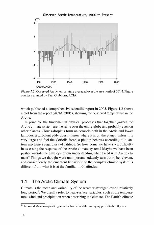
Figure 1.2: Observed Arctic temperature averaged over the area north of 60◦N. Figurecourtesy granted by Paul Grabhorn, ACIA.

which published a comprehensive scientific report in 2005. Figure 1.2 showsa plot from the report (ACIA, 2005), showing the observed temperature in theArctic.

In principle the fundamental physical processes that together govern theArctic climate system are the same over the entire globe and probably even onother planets. Clouds-droplets form on aerosols both in the Arctic and lowerlatitudes, a turbulent eddy doesn’t know where it is on the planet, unless it isvery large and feel the Coriolis force, a photon behaves according to quan-tum mechanics regardless of latitude. So how come we have such difficultyin assessing the response of the Arctic climate system? Maybe we have beenpushed outside the envelope of our understanding when faced with Arctic cli-mate? Things we thought were unimportant suddenly turn out to be relevant,and consequently the emergent behaviour of the complex climate system isdifferent from what it is at the familiar mid-latitudes.

1.1 The Arctic Climate SystemClimate is the mean and variability of the weather averaged over a relativelylong period1. We usually refer to near-surface variables, such as the tempera-ture, wind and precipitation when describing the climate. The Earth’s climate

1The World Meteorological Organisation has defined the averaging period to be 30 years.

14

Sunlight

Infrared radiation

Winds

Sea-ice

Currents

EntrainmentTurbulence

Snow/Tundra

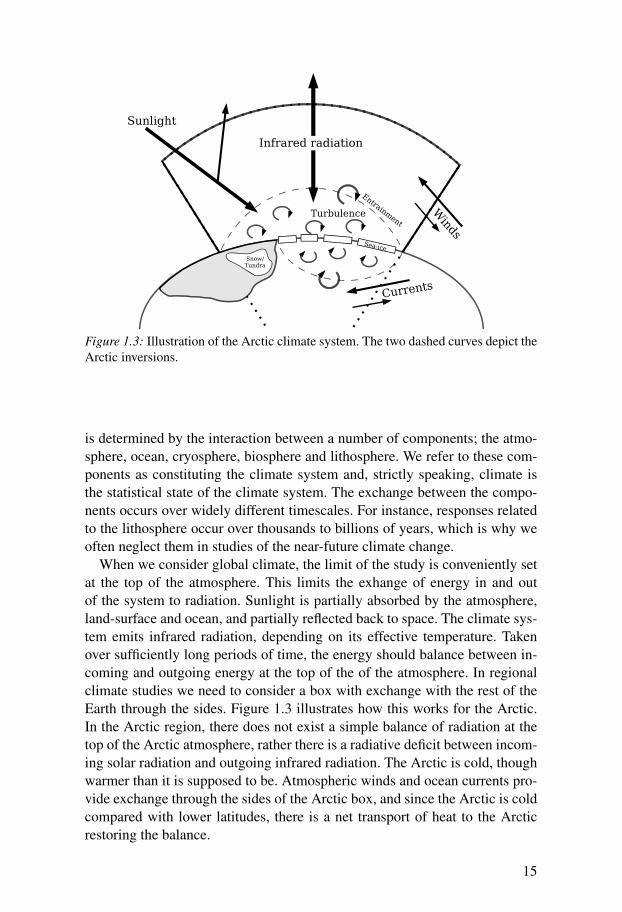
Figure 1.3: Illustration of the Arctic climate system. The two dashed curves depict theArctic inversions.

is determined by the interaction between a number of components; the atmo-sphere, ocean, cryosphere, biosphere and lithosphere. We refer to these com-ponents as constituting the climate system and, strictly speaking, climate isthe statistical state of the climate system. The exchange between the compo-nents occurs over widely different timescales. For instance, responses relatedto the lithosphere occur over thousands to billions of years, which is why weoften neglect them in studies of the near-future climate change.

When we consider global climate, the limit of the study is conveniently setat the top of the atmosphere. This limits the exhange of energy in and outof the system to radiation. Sunlight is partially absorbed by the atmosphere,land-surface and ocean, and partially reflected back to space. The climate sys-tem emits infrared radiation, depending on its effective temperature. Takenover sufficiently long periods of time, the energy should balance between in-coming and outgoing energy at the top of the of the atmosphere. In regionalclimate studies we need to consider a box with exchange with the rest of theEarth through the sides. Figure 1.3 illustrates how this works for the Arctic.In the Arctic region, there does not exist a simple balance of radiation at thetop of the Arctic atmosphere, rather there is a radiative deficit between incom-ing solar radiation and outgoing infrared radiation. The Arctic is cold, thoughwarmer than it is supposed to be. Atmospheric winds and ocean currents pro-vide exchange through the sides of the Arctic box, and since the Arctic is coldcompared with lower latitudes, there is a net transport of heat to the Arcticrestoring the balance.

15

The emitted infrared radiation to space is proportional to the fourth powerof the Earths’s effective temperature. It is the temperature Earth would haveif it had no atmosphere and acted like a black body, absorbing all the in-coming radiation received at its surface and reradiating it all back to space.The effective temperature of the Earth as a whole is about -17◦C. Had it notbeen for the atmospheres greenhouse effect the planet would have this averagetemperature. In this scenario the temperature would vary wildly, by hundredsof degrees, between day and night, summer and winter. Popularly speaking,the greenhouse effect warms the lower parts of the atmosphere by absorbingsome of the infrared radiation and emitting it in all directions, including backtoward the surface. Water vapor is the most important greenhouse gas, as itaccounts for about one third of the total greenhouse effect. Other importantgreenhouse gases are carbon dioxide, ozone, methane and nitrous oxide. Inaddition clouds, which mostly consist of water, are important absorbers of in-frared radiation. The main components of the atmosphere, molecular nitrogen,oxygen and argon, are not greenhouse gases.

If we consider the Arctic surface temperature things get more complicated.Here a large number of physical processes are at play within the atmosphere,ocean, sea-ice and ground. The major components are the incoming and re-flected solar radiation, the downward infrared radiation emitted from the at-mospheric greenhouse gases, infrared radiation emitted by the surface, con-ducted heat from the ocean, sea-ice, snow, tundra and the ground, and finally,the exchange of heat to and from the atmosphere by atmospheric motion. Thelatter is a main topic in the present thesis. Exchange at the surface by atmo-spheric motion is often referred to as turbulent exchange. It consists of twocomponents; the sensible heat flux is caused by mixing of air with differenttemperatures and is directed from warm to cold, while the latent heat fluxconsists of the latent heat of evaporation usually directed from the surface tothe atmosphere. The latent heat flux is very small in the Arctic (Persson et al.2002) because the atmosphere can hold very little water at low temperatures.

Exchange between the atmosphere and the surface has to overcome the Arc-tic temperature inversion, one of the major features of the Arctic atmosphere.It is generated as relatively warm air from the midlatitudes moves into the Arc-tic region aided by low-pressure systems. Here the intruding warm air slowlyrises, or slides up, over the cold and dense air close to the surface. The latter iskept cold by the radiative deficit. In wintertime, the temperature is observed toincrease with height on average by roughly 10◦C in the lowermost kilometer(e.g. Kahl et al. 1996). In a well-mixed dry atmosphere the temperature wouldhave decreased by the same amount, due to the adiabatic cooling with height.A similar inversion is present in the uppermost ocean, where relatively freshand cold water resides in a layer of 50-100 meters above the saline, warm, andhence denser water of North Atlantic origin.

The two Arctic inversions effectively shield the Arctic surface from the freeatmosphere and deep ocean. The reason is that the air is stably stratified: A

16

small parcel of air from the free atmosphere is potentially less dense than asmall parcel close to the ground. By ’potential density’ we mean the densitygiven the same pressure without exchange of heat with the surroundings (anadiabatic process). If we were to try to move the parcel from the free atmo-sphere into the boundary layer we would feel a positive buoyancy force, whichwould attempt to move the parcel back to its original position. In other words;it takes energy to mix over an inversion. On the other hand, the inversion isthere because there is a lack of, or only very weak, mixing across it. Verticalexchange of heat in the Arctic is in sharp contrast to the tropics, where a slightwarming of the surface will result in a warming throughout the troposphere.Deep convective cells convey the heat away from the surface in impressivethunderstorms. In fact, the warming in the upper parts of the troposphere willbe larger than at the surface, due to the simultaneous release of latent heat.We shall return to these differences between the Arctic and the rest of Earthin Chapter 5, where the issue of polar amplification is addressed.

1.2 Boundary Layers and TurbulenceThe Earth’s atmosphere is traditionally divided into a number of layers inthe vertical. The lower part, which is denoted the boundary layer, is looselydefined as being influenced by the surface on a timescale of an hour. For ex-ample, if the surface temperature were to change it would be felt within theentire boundary layer in roughly one hour. Typically, the boundary layer issaid to encompass the lowest kilometer of the atmosphere, a value often citedin textbooks. However, the depth of the boundary layer may vary from just afew meters during calm clear nights up to several kilometers on sunny summerdays.

Once in a while, we can observe the boundary layer without a need forsofisticated instrumentation. One such example is the formation of shallowfogs around sunset. Here the evaporating moisture from the ground is trappedwithin a very thin layer, while at the same time the temperature drops, suchthat the humidity reaches saturation. These shallow and stably stratifiedboundary layers, not the fog itself, are the main focus of this thesis. Anotherprominent example is the fair-weather cumulus clouds that form in theafternoon over land in the upper part of the boundary layer. Here parcels ofwarm and moist buoyant air rise from the surface as they are less heavy thantheir environment. As they rise, they cool due to the falling pressure withheight, such that at some point a small cloud may form.

Within the boundary layer the flow is dominated by turbulence. Most peo-ple know turbulence from commercial flights, where it is referred to as ’holesin the air’. This labelling is a misconception. In fact the atmosphere containsno voids, rather the sensation of falling into a hole is caused by small down-ward windgusts. The human fear of falling spawns an immediate response,

17

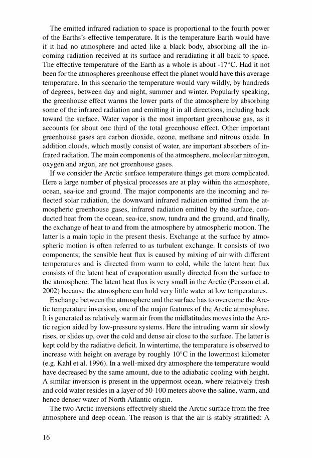
Figure 1.4: Drawing by Leonardo da Vinci of turbulent eddies generated by waterflowing into a basin. The drawing was obtained from http://www.visi.com/ reuteler/.

even though the drop of commercial aircrafts seldom exceeds one meter. Tur-bulence is also responsible for the sound of blowing wind and the rapid dis-persion of odours. However, the most important influences of turbulence onour lives are invisible to the naked eye.

Turbulent flows, governed by the fundamental laws of physics and welldescribed by the laws of mechanics, remain one of the fundamental unsolvedproblems in physics. Most scientist even agree that it is probably an unsolvableproblem, at least within our present understanding.

The modern theories and discoveries of turbulence were made for the mostpart more than fifty years ago in Russia by prominent scientist such as Landau,Kolmogorov and Monin to mention a few. Earlier scientific contributions fromReynolds, Richardson and Prandtl should be included. Their findings in turnbuild on the work of Newton, Bernoulli and Euler. Possibly they found theirinspiration in the artistic drawing by Leonardo da Vinci, which date aroundthe year 1500 (Figure 1.2). We can only speculate on which insights Leonardopossessed concerning the nature of turbulence. The parodic poem2 by LewisFry Richardson from around 1920 nicely illustrates the fractal nature of tur-bulence:

"Big whorls have little whorlsthat feed on their velocity;

2The poem is based on the Anglo-Irish priest and satirist Jonathan Swift’s poem on infinity:’So, nat’ralists observe, a flea; Hath smaller fleas that on him prey; And these have smaller yetto bite ’em; And so proceed ad infinitum; Thus every poet, in his kind, Is bit by him that comesbehind.’

18

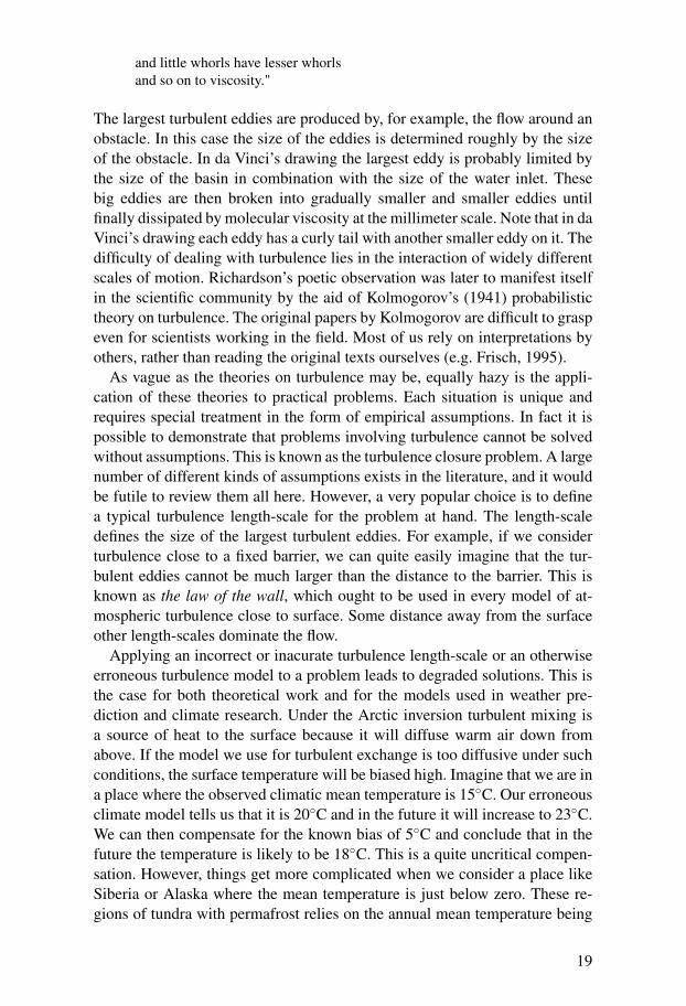
and little whorls have lesser whorlsand so on to viscosity."

The largest turbulent eddies are produced by, for example, the flow around anobstacle. In this case the size of the eddies is determined roughly by the sizeof the obstacle. In da Vinci’s drawing the largest eddy is probably limited bythe size of the basin in combination with the size of the water inlet. Thesebig eddies are then broken into gradually smaller and smaller eddies untilfinally dissipated by molecular viscosity at the millimeter scale. Note that in daVinci’s drawing each eddy has a curly tail with another smaller eddy on it. Thedifficulty of dealing with turbulence lies in the interaction of widely differentscales of motion. Richardson’s poetic observation was later to manifest itselfin the scientific community by the aid of Kolmogorov’s (1941) probabilistictheory on turbulence. The original papers by Kolmogorov are difficult to graspeven for scientists working in the field. Most of us rely on interpretations byothers, rather than reading the original texts ourselves (e.g. Frisch, 1995).

As vague as the theories on turbulence may be, equally hazy is the appli-cation of these theories to practical problems. Each situation is unique andrequires special treatment in the form of empirical assumptions. In fact it ispossible to demonstrate that problems involving turbulence cannot be solvedwithout assumptions. This is known as the turbulence closure problem. A largenumber of different kinds of assumptions exists in the literature, and it wouldbe futile to review them all here. However, a very popular choice is to definea typical turbulence length-scale for the problem at hand. The length-scaledefines the size of the largest turbulent eddies. For example, if we considerturbulence close to a fixed barrier, we can quite easily imagine that the tur-bulent eddies cannot be much larger than the distance to the barrier. This isknown as the law of the wall, which ought to be used in every model of at-mospheric turbulence close to surface. Some distance away from the surfaceother length-scales dominate the flow.

Applying an incorrect or inacurate turbulence length-scale or an otherwiseerroneous turbulence model to a problem leads to degraded solutions. This isthe case for both theoretical work and for the models used in weather pre-diction and climate research. Under the Arctic inversion turbulent mixing isa source of heat to the surface because it will diffuse warm air down fromabove. If the model we use for turbulent exchange is too diffusive under suchconditions, the surface temperature will be biased high. Imagine that we are ina place where the observed climatic mean temperature is 15◦C. Our erroneousclimate model tells us that it is 20◦C and in the future it will increase to 23◦C.We can then compensate for the known bias of 5◦C and conclude that in thefuture the temperature is likely to be 18◦C. This is a quite uncritical compen-sation. However, things get more complicated when we consider a place likeSiberia or Alaska where the mean temperature is just below zero. These re-gions of tundra with permafrost relies on the annual mean temperature being

19

below zero. Our erroneous model would not have the tundra in first place. Orconsider the sea-ice extent in a model that has such a bias. Unfortunately, abias of 5◦C is not uncommon in climate models and for the Arctic region, it isoften much larger.

1.3 Major Questions AddressedThis thesis is based on the papers I-V listed in the beginning. Out of necessity,these are written at a scientific level which is difficult to approach for mostreaders and they further contain many details of little interest to anyone butscientists in the specific fields. I therefore decided to let the following fourchapters treat general problems of meteorology, all of which can be foundin textbooks in use for under-graduate and graduate level teaching. Obviously,papers I-V do not cover the width and breadth of these fundamental questions,rather, they should be viewed as small contributions to the respective scientificfields.

1. The most important atmospheric motion, that on average contain themost energy, are the large-scale synoptic, or weather, and the small-scale turbulent boundary layer scales. Each scale has a certain amountof energy associated with it. It is fundamental to many present-dayobservational techniques and to many atmospheric models that thesynoptic- and boundary layer scales are separated by a spectral en-ergy ’gap’ at the intermediate mesoscales. The problem, and the ex-istence of such a gap is discussed in Chapter 2.

2. Turbulence under stable stratification has long been thought to de-cay beyond a certain limit, the critical Richardson number (Richard-son,1920). Here the stratification becomes so strong that turbulenteddies will not be able to exist. Chapter 3 brings forth new evidencethat this picture needs to be refined. Rather than a non-turbulent state,super-critical turbulence appears weak, though active.

3. Modeling of atmospheric turbulence under stable stratification is amajor problem in numerical weather forecasting and climate simu-lations. It is most often based on work by Obukhov (1946), wherethe vertical turbulent fluxes of momentum and heat are describedby stability functions of the turbulent fluxes themselves. An alter-native approach is sketched in Chapter 4, where instead the gradientRichardson number is used.

4. Historic observations and climate model simulations indicate thatthe Arctic region is more sensitive to external climate forcing thanthe rest of the Earth, the Arctic amplification phenomenon. A com-mon hypothesis explaining Arctic amplification is related to the de-creasing reflectivity of the surface in a warming scenario as snowand ice melts. Chapter 5 questions the importance of this hypothesis

20

and widens the discussion to include the effect of stable stratificationclose to ground on climate sensitivity.

21

2. Atmospheric Scales of Motion

Atmospheric motion occur on all scales, with an upper limit dictated by thesize of Earth and a lower given by the molecular viscosity of air. In practicethis means scales from millimeters to tens of thousands of kilometers. A com-prehensive understanding of the atmosphere involves some kind of treatmentof all these scales of motion, including their interaction. We usually dividethe atmospheric motions into different categories as discussed in Paper IV:Planetary, synoptic, mesoscale and boundary-layer scales. Planetary scale mo-tions of a magnitude which is a fraction of the Earths circumference and areclosely linked with the temperature and pressure distributions. Therefore, theyare usually characterized by their planetary or hemispheric wavenumbers; forinstance motions with a positive pressure anomaly in Asia and negative inNorth America is at wavenumber one. Another example is the Arctic Oscilla-tion which, roughly speaking, is the pressure difference between the high- andthe mid-latitudes. The synoptic scales are the typical sizes of low- and high-pressure weather systems (Bjerknes and Solberg, 1922; Holton, 2004). Theboundary-layer scales range from small-scale turbulence to eddies over thedepth of the boundary layer. The mesoscales, meaning the scales in between,are characterized by a number of phenomena such as fronts, gravity waves,thunderstorms, wind jets etc. The mesoscales tend to be defined in terms ofthe adjacent boundary-layer and synoptic scales, rather than in their own right(Paper IV).

Other classifications of the atmospheric spectrum of motions exist. For in-stance Stull (1988) distinguished between macro-, meso- and micro-scales, indescending order, while Thunis and Bornstein (1996) suggested three subdi-visions of each scale to achieve a total of nine classes. There exists no clear-cut definitions of the limits between any of the scales and classes. The mostpoorly defined limits are those related to the mesoscale and boundary-layerscales (Paper IV). Tentative limits on the scales are given in Figure 2.1. In-deed, while the synoptic and planetary scales each span roughly one orderof magnitude, the mesoscales contain three and the boundary-layer scales en-compass motion over six orders of magnitude.

Each scale of motion has a certain amount of kinetic energy associated withit. Deriving an average energy spectrum from atmospheric winds reveal sev-eral things about the atmospheric system. Spectra come in two kinds. Fre-quency spectra are obtained from a time-series of observations at a point,while wavenumber spectra can be obtained from for example aircraft ob-

23

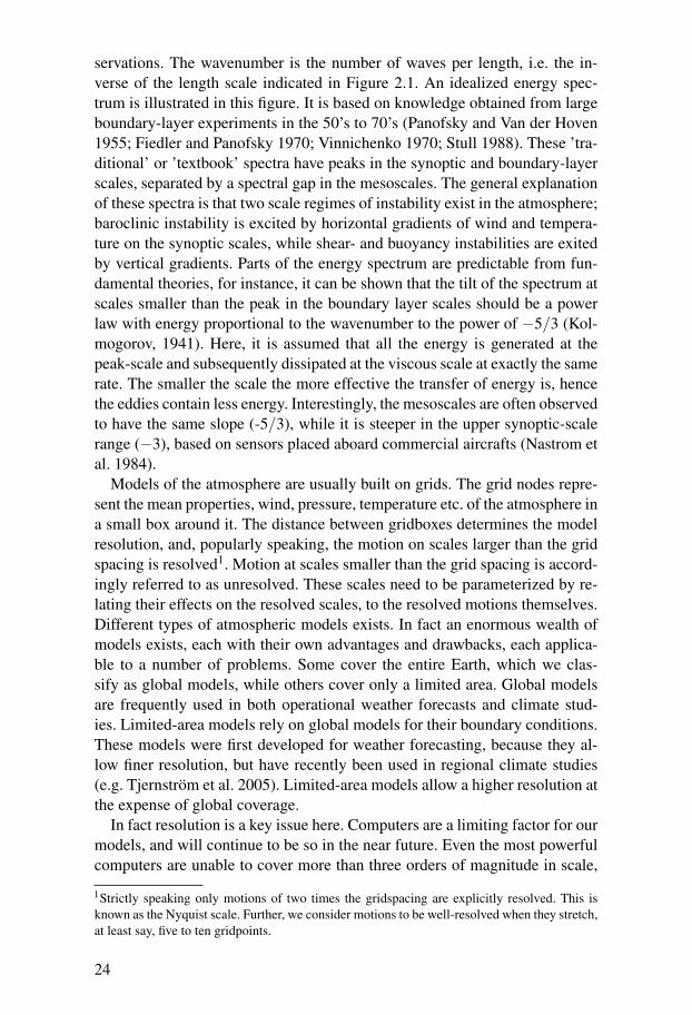
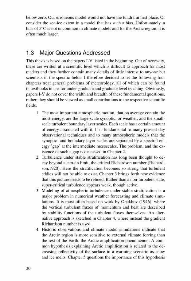
servations. The wavenumber is the number of waves per length, i.e. the in-verse of the length scale indicated in Figure 2.1. An idealized energy spec-trum is illustrated in this figure. It is based on knowledge obtained from largeboundary-layer experiments in the 50’s to 70’s (Panofsky and Van der Hoven1955; Fiedler and Panofsky 1970; Vinnichenko 1970; Stull 1988). These ’tra-ditional’ or ’textbook’ spectra have peaks in the synoptic and boundary-layerscales, separated by a spectral gap in the mesoscales. The general explanationof these spectra is that two scale regimes of instability exist in the atmosphere;baroclinic instability is excited by horizontal gradients of wind and tempera-ture on the synoptic scales, while shear- and buoyancy instabilities are exitedby vertical gradients. Parts of the energy spectrum are predictable from fun-damental theories, for instance, it can be shown that the tilt of the spectrum atscales smaller than the peak in the boundary layer scales should be a powerlaw with energy proportional to the wavenumber to the power of −5/3 (Kol-mogorov, 1941). Here, it is assumed that all the energy is generated at thepeak-scale and subsequently dissipated at the viscous scale at exactly the samerate. The smaller the scale the more effective the transfer of energy is, hencethe eddies contain less energy. Interestingly, the mesoscales are often observedto have the same slope (-5/3), while it is steeper in the upper synoptic-scalerange (−3), based on sensors placed aboard commercial aircrafts (Nastrom etal. 1984).

Models of the atmosphere are usually built on grids. The grid nodes repre-sent the mean properties, wind, pressure, temperature etc. of the atmosphere ina small box around it. The distance between gridboxes determines the modelresolution, and, popularly speaking, the motion on scales larger than the gridspacing is resolved1. Motion at scales smaller than the grid spacing is accord-ingly referred to as unresolved. These scales need to be parameterized by re-lating their effects on the resolved scales, to the resolved motions themselves.Different types of atmospheric models exists. In fact an enormous wealth ofmodels exists, each with their own advantages and drawbacks, each applica-ble to a number of problems. Some cover the entire Earth, which we clas-sify as global models, while others cover only a limited area. Global modelsare frequently used in both operational weather forecasts and climate stud-ies. Limited-area models rely on global models for their boundary conditions.These models were first developed for weather forecasting, because they al-low finer resolution, but have recently been used in regional climate studies(e.g. Tjernström et al. 2005). Limited-area models allow a higher resolution atthe expense of global coverage.

In fact resolution is a key issue here. Computers are a limiting factor for ourmodels, and will continue to be so in the near future. Even the most powerfulcomputers are unable to cover more than three orders of magnitude in scale,

1Strictly speaking only motions of two times the gridspacing are explicitly resolved. This isknown as the Nyquist scale. Further, we consider motions to be well-resolved when they stretch,at least say, five to ten gridpoints.

24

1 km 1.000 km 10.000 km

Boundary-layerscales

MesoscalesSynoptic

scalesPlanetary

scales

Global models

Limited-area models

Computer simulations'Traditional'

energy-spectrum

1 mm

Figure 2.1: Atmospheric scales of motion. The physical limits and the shape of theenergy-spectrum are tentative.

while two orders are more common (Figure 2.1). For example the EuropeanCenter for Medium Range Weather Forecasts (ECMWF) global model, one ofthe finest models for weather prediction as of today, is able to resolve at bestbetween one and 799 waves around the Equator. The problem will continueto exist for a long time because a doubling of the resolution results in a ten-fold increase in computational loading. Hence going from three to four ordersof magnitude scale coverage requires a thousand times more computationalpower. The same limitations apply to fine-scale computer simulations, whichare frequently used to study boundary-layer scale turbulence. For example di-rect numerical simulations (DNS) carry gridspacings of a few millimeters, andhence are unable to deal with a volume larger than, say, a few cubic meters(Figure 2.1). Large-eddy simulations (LES) parameterize the small-scale tur-bulence and consider only the largest turbulent eddies. Even so they seldomcover more than two orders of magnitude and are therefore unable to emu-late interactions with the mesoscales to any significant extent. Consequently,our knowledge of the atmosphere based on computer models and simulationsremains patchy. We can only simulate a small range of scales at a time, forinstance the model used in Paper I spanned 1-100 km. The larger and smallerscales of motion are either handled though boundary conditions, neglected orparameterized. For example, the boundary conditions for limited area modelsare usually obtained from global models, extending the resolved scales of mo-tion, while LES/DNS often use cyclic boundary conditions whereby motionover scales larger than the domain are neglected.

25

It was suggested by Osborne Reynolds (1848-1912) to divide turbulentflows into two parts; the mean and the turbulent deviation from the mean.Summing the two parts we retain the original flow. Formally, we write theReynolds decomposition of a single variable as:

u(t) = u+u(t)′, (2.1)

where x, y and z are spatial dimensions and t is time. The overline defines thetime average of the variable and the prime the temporal deviations from themean. It follows that u′ = 0. We shall further use standard notation, such thatu is the wind in the x-direction, v is the wind in the y-direction and w is thevertical wind. Reynolds averaging is used for analyzing observations and inthe theoretical derivation of equations for the mean-flow and the higher ordermoments, including velocity variance u′u′ and vertical fluxes of momentumand heat, u′w′ and w′θ ′.

The rationale behind the use of global and limited-area models, which of-ten only resolve the global and synoptic scales, is that the unresolved motionthat is important can be described in terms of the resolved scales, aided by theReynolds decomposition. That is, given a certain state of the resolved scalesthe unresolved scales will respond, at least statistically, in a predictable way.If so, we can create parameterizations, based on theory and observations, thatreplace the unresolved scales (e.g. Paper II and Paper III). The development ofsuch parameterizations is aided by the presence of the spectral gap discussedabove. The spectral gap allows separation of the boundary layer scales fromthe synoptic scales. If we account for everything from the smallest scales upto the peak of the boundary layer scales, including more scales will not addsignificantly to the results. In that case, the same parameterization for unre-solved scales can be used in any model with gridspacings between 1 and 1.000km, because these scales are not all that important. If, on the other hand, thespectral gap does not exist, the necessary parameterization will depend on theresolution (Duynkerke, 1998).

As simple as it may seem, the Reynolds decomposition (2.1) offers greatpractical difficulties when applied to observations (Paper II). The source oftrouble is the time-average2 that has to be performed when separating themean-flow from the deviations. The expression ’one man’s turbulence is an-other’s mean-flow’ certainly applies. If there is gap in the energy spectrumit should not matter much, as long as we have included the boundary layerscales. Spokesmen for a shorter time-window argue that the mesoscale mo-tion should be avoided as it does not follow any laws or simple rules (Mahrtand Vickers 2003). The critics say that we need to investigate the influence

2In principle, an ensemble average over all possible realisations of the experiment has to betaken. This is most inconvenient, since the atmosphere only offers us one of these possible real-isations, and in practice we therefore only consider time- or space-averages, aided by Taylor’shypothesis of ’frozen’ turbulence.

26

10−6

10−5

10−4

10−3

10−2

10−1

100

101

10−3

10−2

10−1

100

Frequency (Hz)

nSu (

m2 s

−2

(b)

) Inertial

Diurnal

Week Oden 35 mMast 18 mSonic USonic VSonic W

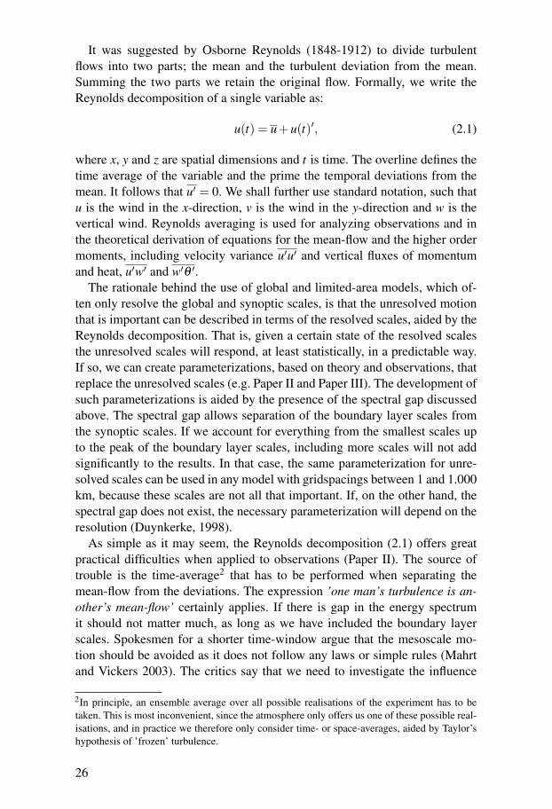
Figure 2.2: Frequency energy-spectrum obtained during the AOE-2001 campaign.The boundary-layer scales are divided into along wind, u, cross wind, v, and vertical,w, deviations from the mean. These are measured by the sonic anemometers. Note thatthe smallest scales are on the right, opposite to Figure 2.1. See Paper IV for furtherdetails.

of the mesoscales as they are potentially important in global models (Beljaarsand Viterbo 1998; Viterbo et al. 1999; Beljaars 2001; Chapter 4).

While the traditional power spectra (Panofsky and Van der Hoven 1955;Fiedler and Panofsky 1970; Vinnichenko 1970; Stull 1988) exhibit a clearspectral gap, measurements from the Arctic summer boundary layer indicatea plateau in the mesoscale range (Figure 2.2; Paper IV). At times there isnot even a plateau, and the mesoscale motion appears to enhance the surfaceturbulence. Further, there are indications that mixing occurs from the free at-mosphere into the boundary layer during such events. The mixing events aremore frequent when the temperature difference between the surface and thefree atmosphere is larger, i.e. the more stable the stratification is. Two majorintrusions of warm air from lower latitudes set the background for such ac-tivity. One can only speculate where the mesoscale energy comes from. PaperIV suggests gravity waves and very shallow mesoscale fronts confined to thelowest part of the atmosphere. These results provide some support for recenttheories that gravity waves in the free atmosphere may influence surface turbu-lence if there is a continuous stratification between the boundary layer and thefree atmosphere (Zilitinkevich 2002). Further, paper I presents simulations ofgravity waves emerging from openings in the sea-ice. These waves are shownto cause elevated mixing of this type within the model framework. The wavesare, however, standing and should be distinguished from the waves observedin Paper IV which travel past the stationary sensors.

27

It can certainly be debated whether the spectral gap really exists in the sta-bly stratified boundary layer of the Arctic (e.g. Paper IV). It has been arguedthat the central Arctic Ocean is ’the perfect laboratory’ for studies of small-scale turbulence, since there is no topography and the surface is relativelyhorizontally homogeneous (Grachev et al. 2005). These are basic assumptionsoften violated at other experimental sites. More so, they are often blamed forbeing the sources of unwanted or disturbing mesoscale motion. Even so PaperIV finds evidence for frequent mesoscale activity, both features resemblinggravity-waves and mesoscale fronts apparently thriving under the Arctic in-version.

28

3. Stably Stratified Boundary Layers

In the 1970’s and 80’s the stably stratified boundary layer was, more or less,put aside for studies of the unstable convective boundary layer. There can beseveral reasons for this neglect. The unstable boundary layer is much deeper,characterized by larger fluxes of heat, momentum and pollutants, occurs com-fortably during daytime, and is in general more spectacular than its stablecounterpart. Further, the computer simulations at that time did not permit thestudy of the stable boundary layer due to the fine resolution necessary. Fur-ther, long-standing theories predicted that if the boundary layer was very sta-ble, beyond a certain limit to be explained below, turbulence would decay(Richardson 1920; Chandrasekhar 1961; Howard 1961; Miles 1961; Miles1986). These results are repeated in most textbooks on the subject. The the-ories are now being called into question by observations (Paper II) as wellas from a theoretical and modeling perspective (e.g. Zilitinkevich et al. 2007;Paper III). We shall take a closer look at this debate.

When light air reside above more dense air, we say that the atmosphere isstably stratified. Most of the atmosphere is in fact stably stratified. When theopposite occurs the atmosphere is out of balance and will attempt to overturnin order to restore the balance. We refer to this situation as the atmospherebeing unstable. We have already touched upon these phenomena in the intro-duction - here we shall proceed in a more formal fashion. Unfortunately, theabove notions on the stability are not exactly true but require some refinement.Because pressure decreases with altitude the density of a parcel of air will alsodecrease as we move it upward, at the same time as the temperature decreasesdue to the expansion. For a dry atmosphere in balance the temperature will de-crease by roughly 1◦C per 100 m altitude, less if the atmosphere is saturatedwith water vapor. What determines whether the atmosphere is stable or unsta-ble is if the density of a parcel of air is smaller or larger than its surroundingswhen perturbed from its initial position. This means that the dry atmosphereis stable if the temperature decreases by less than 1◦C per 100 m and unstableif the gradient somewhere is steeper. For these reasons meteorologists find itconvenient to define variables that are conserved under vertical motion. Manydifferent definitions exist, here it suffices to define the potential temperature:

θ = T(

pp0

)− Rcp

, (3.1)

where T is the absolute temperature measured in degrees Kelvin, p is theactual pressure, p0 is a reference pressure, 1000 hPa, R is the gas constant and

29

cp is the specific heat capacity of dry air at a constant pressure, respectively.θ is the temperature a parcel of air would achieve if brought to the referencepressure without exchange of heat with the surroundings1.

The potential temperature definition allows us to easily distinguish betweenunstable and stable stratification. If θ increases with height, the stratification isstable and if the potential temperature is higher close to the ground than above,the atmosphere is unstable. If the atmosphere is stable, a parcel released outof equilibrium will oscillate up and down about the equilibrium height. Therate of the oscillation is the famous Brunt-Väisälä frequency, N, given by:

N2 =gθ· ∂θ

∂ z, (3.2)

where g is gravity. Note how N2 increases as the vertical derivative of θ does:The more stably stratified the atmosphere is the faster may it oscillate. If thestratification is unstable, i.e. ∂θ/∂ z < 0, N is imaginary. The physical inter-pretation of an imaginary N is that a parcel brought out of equilibrium in anunstable atmosphere will accelerate away from equilibrium, ultimately result-ing in an overturning of the atmosphere.

Under stably stratified conditions mixing may, however, prevent the parcelfrom returning to its original position. The necessary energy to overcome thestable stratification can be attained from the mean-flow wind-shear. Usually,horizontal shear is negligeble in the boundary layer compared to the verticalshear. Therefore, the total shear can be approximated:

S2 =(

∂U∂ z

)2

+(

∂V∂ z

)2

, (3.3)

where U and V are the components of the mean wind. Note how S has thesame unit of frequency (s−1) as the Brunt-Väisälä frequency.

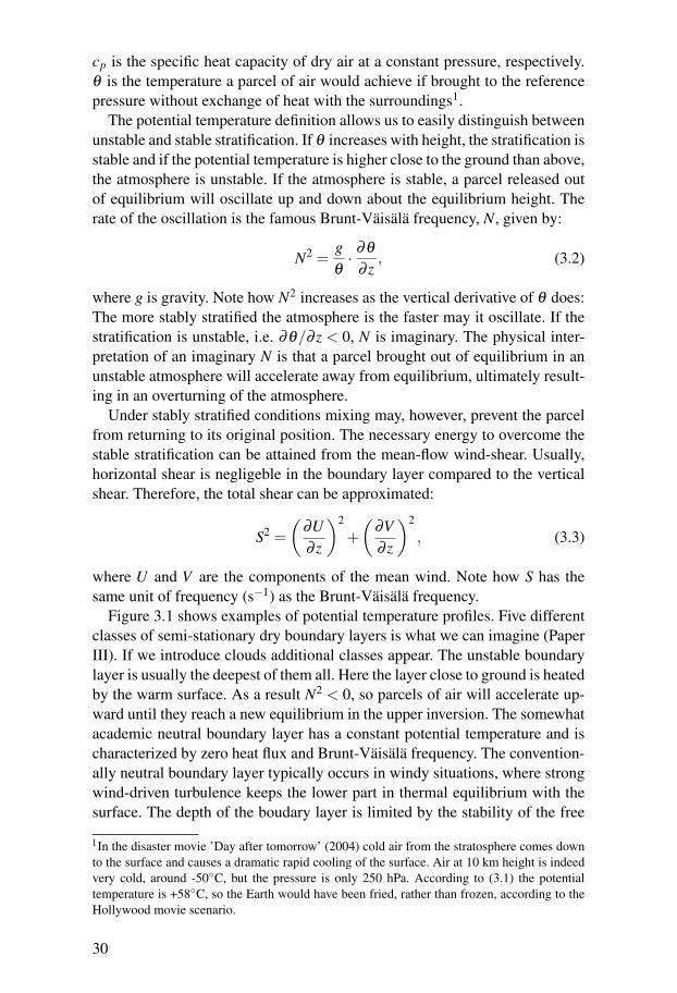
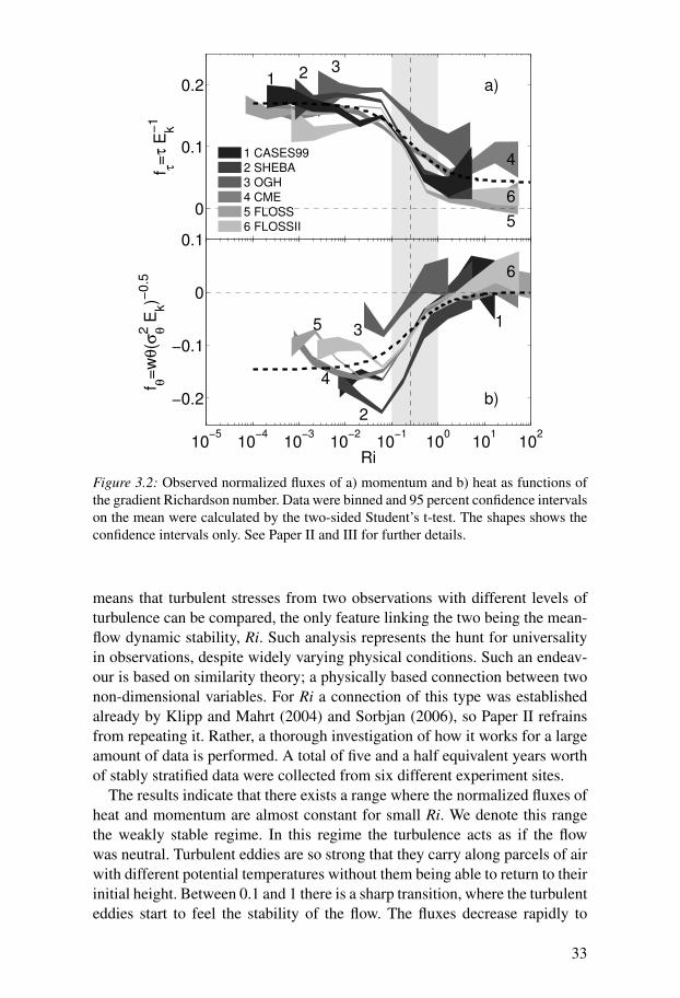
Figure 3.1 shows examples of potential temperature profiles. Five differentclasses of semi-stationary dry boundary layers is what we can imagine (PaperIII). If we introduce clouds additional classes appear. The unstable boundarylayer is usually the deepest of them all. Here the layer close to ground is heatedby the warm surface. As a result N2 < 0, so parcels of air will accelerate up-ward until they reach a new equilibrium in the upper inversion. The somewhatacademic neutral boundary layer has a constant potential temperature and ischaracterized by zero heat flux and Brunt-Väisälä frequency. The convention-ally neutral boundary layer typically occurs in windy situations, where strongwind-driven turbulence keeps the lower part in thermal equilibrium with thesurface. The depth of the boudary layer is limited by the stability of the free

1In the disaster movie ’Day after tomorrow’ (2004) cold air from the stratosphere comes downto the surface and causes a dramatic rapid cooling of the surface. Air at 10 km height is indeedvery cold, around -50◦C, but the pressure is only 250 hPa. According to (3.1) the potentialtemperature is +58◦C, so the Earth would have been fried, rather than frozen, according to theHollywood movie scenario.

30

N 20

N 2≈0

N 20

UnstableNeutral Conv. Neutral

Nocturnal Long-lived

Potential Temperature

Hei

ght

Figure 3.1: Idealized potential temperature profiles for five classes of dry unstable,neutral and stably stratified boundary layers.

atmosphere, generating the upper inversion with a large N2. The nocturnal sta-ble boundary layer forms after sunset over land due to the radiative coolingof the surface. Finally, the long-lived stable boundary layer develops againststable stratification, while loosing heat at the surface. These boundary layerstypically occur at high latitudes and over land during winter. Note how allboundary layer classes, except the truly neutral, contain stably stratified parts.In addition most of the free atmosphere and the majority of the oceans arestably stratified, highlighting the need of a better understanding of turbulencein stably stratified conditions.

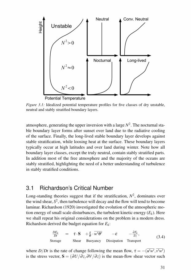
3.1 Richardson’s Critical NumberLong-standing theories suggest that if the stratification, N2, dominates overthe wind shear, S2, then turbulence will decay and the flow will tend to becomelaminar. Richardson (1920) investigated the evolution of the atmospheric mo-tion energy of small scale disturbances, the turbulent kinetic energy (Ek). Herewe shall repeat his original considerations on the problem in a modern dress.Richardson derived the budget equation for Ek:

DEkDt = τ ·S + g

θ·w′θ ′ −ε − ∂Fk

∂ z ,

Storage Shear Buoyancy Dissipation Transport(3.4)

where D/Dt is the rate of change following the mean flow, τ = −(u′w′,v′w′)is the stress vector, S = (∂U/∂ z,∂V/∂ z) is the mean-flow shear vector such

31

that S · S = S2, g is gravity, ε is the dissipation rate and Fk is the verticaltransport of turbulent kinetic energy. Here we shall not consider the verticaltransport term. Equation (3.4) states that the rate of change of Ek is a balancebetween the shear production, buoyancy conversion/production and viscuousdissipation. The shear production is usually positive, while the buoyancy termis negative in stable- and positive in unstable stratification. Buoyancy in stablestratification is therefore a sink of Ek and is often referred to as a destructiveterm. We find it more appropriate to label it conversion for reasons to be givenbelow. The dissipation term is always negative, but presumably proportionalto E3/2

k (Kolmogorov 1941).Next, Richardson considered a case when Ek was small, but finite, such that

the shear production would not be zero, but sufficiently small that dissipationcan be neglected. The question is then if the turbulence will grow, i.e. whetherDEk/Dt > 0? Following (3.4), this will be the case if:

τ ·S >− gθ·w′θ ′. (3.5)

By defining the eddy conductivity w′θ ′ = −Kh∂θ

∂ z and the eddy viscosityτ = KmS and rewriting (3.5) we get an inequality in non-dimensional ratios:

Km

Kh>

N2

S2 . (3.6)

The entity on the left hand side is known as the turbulent Prandtl number,Pr≡Km/Kh, while the right hand side was later to be known as the Richardsonnumber, Ri ≡ N2/S2, such that the inequality reads:

Pr > Ri. (3.7)

Richardson assumed that Km = Kh such that the necessary condition for tur-bulence to grow can be stated Ri < Ric = 1, where Ric is the critical Richardsonnumber. This means that if the flow stability is weak, Ri < 1, then turbulencewill grow to a level where the production is balanced by dissipation. Con-trary, if Ri > 1 the flow is too stable to support turbulence growth accordingto Richardson’s results. Later theoretical studies have supported Richardson’snotion by other means (Chandrasekhar 1961; Miles 1961; Howard 1961). Ob-servations do support a Pr close to unity in near-neutral conditions, 0.7-0.8most often being reported. However, Pr appears not to be constant, rather ob-servations and computer simulations indicate that it is a function of Ri suchthat Pr(Ri) ∝ Ri, for large Ri (e.g. Zilitinkevich et al. 2007). In this case (3.7)is always satisfied, which means that turbulence will always grow to achievea balance with dissipation.

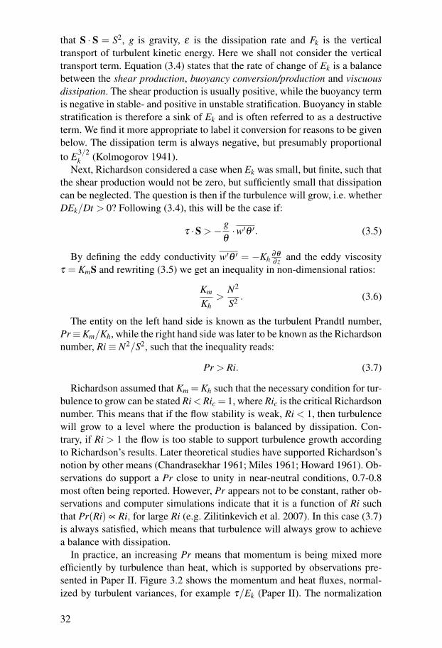
In practice, an increasing Pr means that momentum is being mixed moreefficiently by turbulence than heat, which is supported by observations pre-sented in Paper II. Figure 3.2 shows the momentum and heat fluxes, normal-ized by turbulent variances, for example τ/Ek (Paper II). The normalization

32

1 2 3

4

56

a)

Ri

f τ=τ E

k−1

0

0.1

0.2

1 CASES992 SHEBA3 OGH4 CME5 FLOSS6 FLOSSII

1

2

3

4

5

6

b)

f θ=wθ(

σ θ2 Ek)−0

.5

Ri10−5 10−4 10−3 10−2 10−1 100 101 102

−0.2

−0.1

0

0.1

Figure 3.2: Observed normalized fluxes of a) momentum and b) heat as functions ofthe gradient Richardson number. Data were binned and 95 percent confidence intervalson the mean were calculated by the two-sided Student’s t-test. The shapes shows theconfidence intervals only. See Paper II and III for further details.

means that turbulent stresses from two observations with different levels ofturbulence can be compared, the only feature linking the two being the mean-flow dynamic stability, Ri. Such analysis represents the hunt for universalityin observations, despite widely varying physical conditions. Such an endeav-our is based on similarity theory; a physically based connection between twonon-dimensional variables. For Ri a connection of this type was establishedalready by Klipp and Mahrt (2004) and Sorbjan (2006), so Paper II refrainsfrom repeating it. Rather, a thorough investigation of how it works for a largeamount of data is performed. A total of five and a half equivalent years worthof stably stratified data were collected from six different experiment sites.

The results indicate that there exists a range where the normalized fluxes ofheat and momentum are almost constant for small Ri. We denote this rangethe weakly stable regime. In this regime the turbulence acts as if the flowwas neutral. Turbulent eddies are so strong that they carry along parcels of airwith different potential temperatures without them being able to return to theirinitial height. Between 0.1 and 1 there is a sharp transition, where the turbulenteddies start to feel the stability of the flow. The fluxes decrease rapidly to

33

achieve new nearly constant levels in the very stable regime for Ri > 1. Herethe turbulent stress is reduced to a fraction of the weakly stable regime level,while the turbulent heat flux is statistically indistinguishable from zero. Thelatter does not mean that the heat flux is zero, rather we are unable to measureit such that we can have statistical confidence to conclude that it is non-zero.

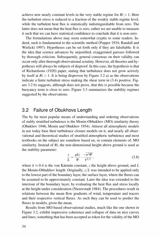
The formulations above may seem somewhat cryptic to some readers. In-deed, such is fundamental to the scientific method (Popper 1934; Randall andWielicki 1997). Hypotheses can be set forth only if they are falsifiable. It isthe idea that science advances by unjustified, exaggerated guesses followedby thorough criticism. Subsequently, general consensus on their validity canoccur only after thorough observational scrutiny. However, all theories and hy-potheses will always be subjects of disproof. In this case, the hypothesis is thatof Richardsons (1920) paper, stating that turbulence does not grow activelyby itself at Ri > 1. It is being disproven by Figure 3.2 a) as the observationsindicate a finite turbulent stress making the shear term in (3.4) positive. Fig-ure 3.2 b) suggests, although does not prove, that this is possible because thebuoyancy term is close to zero. Figure 3.3 summarizes the stability regimessuggested by the observations.

3.2 Failure of Obukhovs LengthThe by far most popular means of understanding and ordering observationsof stably stratified turbulence is the Monin-Obhukhov (MO) similarity theory(Obukhov 1946; Monin and Obukhov 1954). Almost all atmospheric modelsin use today base their turbulence closure models on it, and nearly all obser-vational and theoretical studies of stratified atmospheric turbulence and mosttextbooks on the subject are somehow based on, or contain elements of, MOsimilarity. Instead of Ri, the non-dimensional height above ground is used asthe stability parameter:

zL

=gkzθ

· −w′θ ′

τ3/2 , (3.8)

where k ≈ 0.4 is the von Kármán constant, z the height above ground, and Lthe Monin-Obhukhov length. Originally, z/L was intended to be applied onlyto the lowest part of the boundary layer, the surface layer, where the fluxes canbe assumed to be approximately constant. Later the idea was extended to theinteriour of the boundary layer, by evaluating the heat flux and stress locallyat the height under consideration (Nieuwstadt 1984). The procedures result inrelations between the mean flow gradients of wind, temperature and tracersand their respective vertical fluxes. As such they can be used to predict thefluxes in models, given the mean.

Results from MO-based observational studies, much like the one shown inFigure 3.2, exhibit impressive coherence and collapse of data on nice curvesand lines; something that has been accepted as token for the validity of the MO

34

S2

N2

Unstable Wea

kly

Sta

ble

Very Stable

Tran

sition

Figure 3.3: Schematic of the mean-flow stability range.

similarity theory. Further, the results have supported Richardson’s hypothesisby showing fluxes that tend to zero for large z/L. Unfortunately, data analysisbased on z/L is subject to self-correlation (e.g. Hicks 1978; Mahrt et al. 1998;Baas et al. 2006). Self-correlation occurs in data analysis when the same mea-surement is used on both axes in a plot. For example, a plot of τ/Ek versusz/L would include τ on both axes. Since every measurement has a certain ran-dom error associated with it, these errors will often correlate in such plots togenerate an artificial behaviour of the datapoints. In this case, an erroneouslysmall τ will cause the z/L estimate to be erroneously large, forcing the curvedown towards zero in the very stable regime. The problem of self-correlationis a general one for studies of turbulence data and is very difficult to avoid.Papers II and III lay out a possible path to achieve this goal, though beware, itis not free from trouble and we have yet to see the end of it.

35

4. Models of Atmospheric Turbulence

The smallest scales of motion, the boundary layer scales, are not resolved byglobal and limited-area models. Since they are important for the results theyneed to be included by parameterization as discussed in Chapter 2. Arguably,the most important task of a turbulence parameterization is to provide the sur-face drag to the large-scale flow, and furthermore to provide the atmosphericexchange of heat, moisture and tracers with the surface. With the evolvingdemands on, and complexity of, atmospheric models, the prediction of near-surface variables such as temperature, wind and boundary-layer cloudinessare becoming increasingly important (e.g. Beljaars and Viterbo 1998). Thismeans that correct representation of not only the surface exchange but alsothe vertical structure of the boundary layer is presently in focus. When de-signing and developing a turbulence parameterization scheme several practi-cal problems have to be considered. Ideally, the scheme should be based onphysical principles, and behave as nature does. Unfortunately, the first require-ment is complicated by the turbulence closure problem; even though we knowthe exact equations that describe turbulent flows, we are in general unable tosolve them. Further, even given a good parameterization, modeling the bound-ary layer is a non-linear and coupled problem, which makes the solution verysensitive to even small changes in the scheme. The scheme should functionacross a wide range of conditions, day and night, summer to winter, from Sa-hara to Siberia, and in principle on other planets. Probably, these constraintsare part of the reason why we are reluctant to include new parameterizationsin forecast and climate models. Most models base their parameterization ondevelopments from the 1970s and early 80s.

The properties of the parameterization affect the usefulness of short- tomedium range weather forecasts and climate simulations in different ways.For example short-range weather forecasts for 1 to 2 days are often performedto obtain details at and close to the ground, such as temperature, frost, fogs,strong winds etc., while medium-range weather forecasts for 5 to 10 days willbe most concerned with the development of cyclones and anti-cyclones. In theformer case a well-known problem is so-called run-away cooling. At night,when the surface cools rapidly, these models predict that all turbulence de-cays in such a way that nothing stops further cooling. In the case of medium-range weather forecasts, the life-time of cyclones is largely determined by aphenomenon called boundary layer pumping or Ekman-pumping (e.g. Ekman1902; Beljaars and Viterbo 1998; Beljaars 2001; Holton 2004; Beare 2006).

37

Warm

LCold

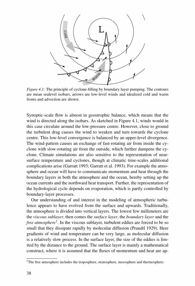
Figure 4.1: The principle of cyclone-filling by boundary layer pumping. The contoursare mean sealevel isobars, arrows are low-level winds and idealized cold and warmfronts and advection are shown.

Synoptic-scale flow is almost in geostrophic balance, which means that thewind is directed along the isobars. As sketched in Figure 4.1, winds would inthis case circulate around the low-pressure centre. However, close to groundthe turbulent drag causes the wind to weaken and turn towards the cyclonecentre. This low-level convergence is balanced by an upper-level divergence.The wind-pattern causes an exchange of fast-rotating air from inside the cy-clone with slow-rotating air from the outside, which further dampens the cy-clone. Climate simulations are also sensitive to the representation of near-surface temperature and cyclones, though at climatic time-scales additionalcomplications arise (Garratt 1993; Garratt et al. 1993). For example the atmo-sphere and ocean will have to communicate momentum and heat through theboundary layers in both the atmosphere and the ocean, hereby setting up theocean currents and the northward heat transport. Further, the representation ofthe hydrological cycle depends on evaporation, which is partly controlled byboundary-layer processes.

Our understanding of and interest in the modeling of atmospheric turbu-lence appears to have evolved from the surface and upwards. Traditionally,the atmosphere is divided into vertical layers. The lowest few millimeters arethe viscous sublayer, then comes the surface layer, the boundary layer and thefree atmosphere1. In the viscous sublayer, turbulent eddies are forced to be sosmall that they dissipate rapidly by molecular diffusion (Prandtl 1929). Heregradients of wind and temperature can be very large, as molecular diffusionis a relatively slow process. In the surface layer, the size of the eddies is lim-ited by the distance to the ground. The surface layer is mainly a mathematicalconstruct, where it is assumed that the fluxes of momentum and heat are ap-

1The free atmosphere includes the troposphere, stratosphere, mesosphere and thermosphere.

38

proximately constant. This assumption permits a particularly simple solution,where the profiles of wind and potential temperature are logarithmic functionsof height. The boundary layer above the surface layer assumes many forms asshown in the previous chapter, cf. Figure 3.1. The free atmosphere is thoughtto not be significantly influenced by turbulence; probably it is more correct tosay that our knowledge of the influence is limited. The division outlined hereis not unique, for example Grachev et al. (2005) named no less than six dif-ferent layers, or regimes as they may be called, for the Arctic stably stratifiedboundary layer.

In atmospheric models this way of dividing the atmosphere is often utilized,as the temperature and winds are only calculated in vertically discrete layers.The viscous sublayer and the surface layer are assumed to exist between thesurface and the first model level, regardless of the height of this level. Thisassumption allows relatively simple boundary conditions from a surface-layermodel. Exchange between levels above the first model level is achieved via theturbulence parameterization. Some models distinguish between the boundarylayer and the free atmosphere. For example, Swedish HIRLAM use one tur-bulent exchange model within the boundary layer and another less diffusivemodel in the free atmosphere. Although a division, with different models inthe surface layer, boundary layer and free atmosphere, may be convenient forthe programmer, there is no physical justification for it. In some cases themodels do not match, and hence discontinuities of the fluxes between the sur-face and the boundary layer occur (Svensson and Holtslag 2007). Ideally, thesame fundamental principles should apply in all three layers, and only themathematical solution technique could possibly differ. Paper III demonstrateshow a turbulence closure model can be extended to all three layers.

For mainly technical reasons, in order to allow long timesteps, the turbu-lent exchange within the boundary layer is described as turbulent diffusionvia the eddy viscosity and eddy conductivity, Km and Kh (see also Chapter3). If a potential temperature gradient exists, the eddy conductivity tells ushow fast turbulent motion will attempt to reduce the gradient. Physically, astrongly turbulent flow is more diffusive than a weakly turbulent flow, so theturbulent diffusivity will depend on the flow. Unfortunately, these quantitiesare not measureable with current observational techniques, rather they have tobe calculated from measured fluxes and gradients. Models of turbulence alsopredict different levels of eddy viscosity and conductivity, given a fixed mean-flow. The response determines the character of the model and ultimately thestate of the boundary layer it will produce. We often speak of more, or less,diffusive models. A model of the former kind will reduce the gradient of thewind between the free atmosphere and the Earth’s surface where it is zero,making the boundary layer deeper than in a less diffusive model. Further, itwill transport heat more efficiently towards the surface under stable stratifica-tion, making the stratification weaker and the surface warmer. Moisture willbe mixed over a deeper layer, possibly obliterating low-level fogs and gener-

39

0 4 8

0

100

200

300

400

500

600

Winds, (ms−1)

Hei

ght,

(m)

−0.08 −0.04 0Momentum fluxes, (m2s−2)

263 265 267 2690

100

200

300

400

500

Potential temperature, (K)

Hei

ght,

(m)

−0.015 −0.01 −0.005 0Heat−flux, (Kms−1)

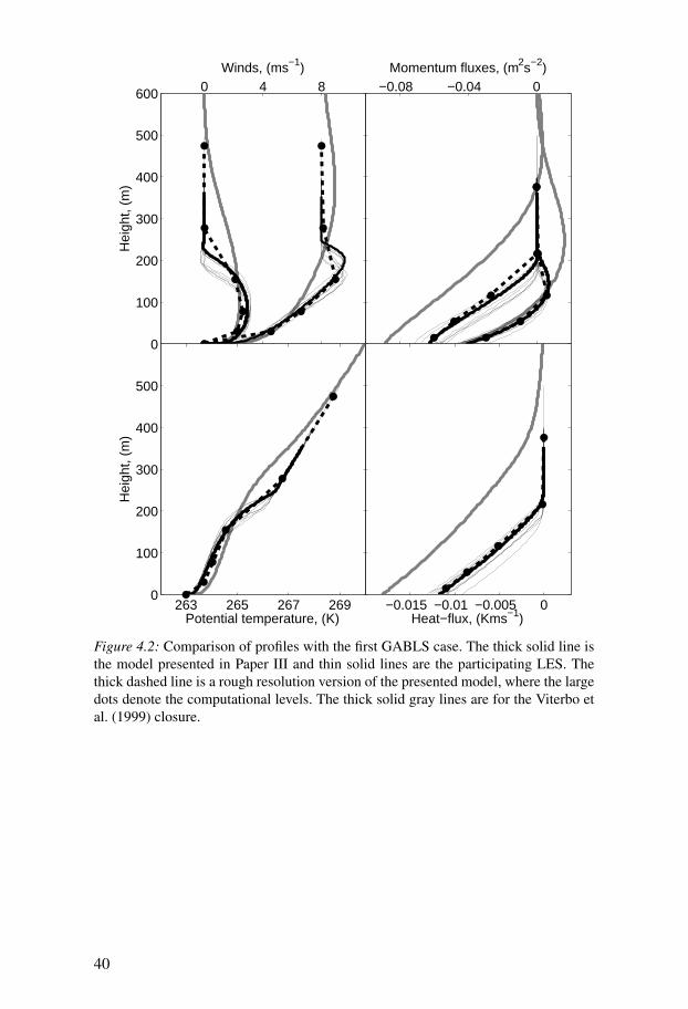
Figure 4.2: Comparison of profiles with the first GABLS case. The thick solid line isthe model presented in Paper III and thin solid lines are the participating LES. Thethick dashed line is a rough resolution version of the presented model, where the largedots denote the computational levels. The thick solid gray lines are for the Viterbo etal. (1999) closure.

40

101 102 103101

102

103

Boundary layer height from LES (m)

Bou

ndar

y la

yer h

eigh

t fro

m 1

D−m

odel

(m)

Truly neutralConventionally neutralNocturnalLong−lived

Figure 4.3: Comparison of boundary layer heights from LES and 1D-models for 90different cases. The boundary layer classes are shown in Figure 3.1. Gray symbols arefor the Viterbo et al. (1999) closure, while black symbols are for the turbulence closuremodel presented in Paper III. The solid line is one-to-one correspondence, while thedotted and dashed lines are 20 and 50 percent difference, respectively.

ating clouds in the upper parts of the boundary layer instead. An example oftwo quite different models is shown in Figure 4.2. The more diffusive turbu-lence closure model (Viterbo et al. 1999) produces a deeper boundary layer,with a stronger downward heat-flux, and more surface stress than the LESand Paper III model. Unfortunately, this first experiment had a fixed surfacetemperature, so the turbulence was not able to alter the surface temperature.Note also that the cross-isobaric massflux, i.e. the area under the left-mostwind-profile, is nearly twice as large for the more diffusive model. While thefirst GABLS case is only considered a weakly stable case, Paper III comparedmodel results with an LES database from the neutral to moderately stableboundary layer (Figure 4.3). The less diffusive model was able to predict theboundary layer height to within 20 percent of the LES. The more diffusivemodel overpredicted boundary layer height for cases shallower than 1 km andunderpredicted the deepest neutral and near-neutral cases.

41

4.1 Boundary Layer ModelsA hierarchy of turbulence closure models for the boundary layer exists. Thesimplest models in use are the first-order closure models, where the fluxesof heat, momentum and tracers are simple functions of the mean-flow windand temperature. A first-order turbulence closure model parameterizes eddyviscosity and eddy conductivity under neutral and stable stratification as (e.g.Louis 1979; Viterbo et al. 1999):

Km = fml2S, (4.1)

Kh = fhl2S,

where fm and fh are non-dimensional functions, l is the turbulent mixinglength and S is the magnitude of the vertical windshear. Most first-order mod-els will have the stability functions and mixing length defined as algebraicfunctions. Both the stability functions and the mixing lengths are important forthe behaviour of the model. Higher-order models include those solving onlythe turbulent kinetic energy equation (3.4), full second-order models solvingnine additional equations (Mellor and Yamada 1974), and so on to infinity.The more complex the model is, the more calculations have to be done andthe more parameters have to be determined. The increasing complexity ofhigher-order models is not necessarily beneficial for their predictive perfor-mance (e.g. Cuxart et al. 2006). The model presented in Paper III includes aprognostic equation for the total turbulent energy, E, which is the sum of theturbulent kinetic and potential energies:

E = Ek +Ep. (4.2)

The turbulent potential energy, which is proportional to the temperaturevariance, is zero for neutral stratification, while Paper II found that at verystrong stability Ep is roughly half of Ek. In contrast, the motion of a pendulumswinging back and forth also consist of both kinetic and potential mechanicalenergy. At the low point all the energy is kinetic, while at the extremes theenergy is all potential. In the absence of friction, the sum of the two will beconstant. In Chapter 3 we demonstrated that the use of the turbulent kineticenergy equation (3.4) may lead to implicit critical Richardson numbers. Asdemonstrated in Paper III, adding the turbulent potential energy to the kineticactually simplifies the problem to solving:

DEDt = τ ·S −γ − ∂FE

∂ z ,

Storage Shear Dissipation Transport(4.3)

where now γ is the total dissipation rate and FE is the total turbulent energytransport. An additional source term appears in unstable situations. Given E,we can calculate the relative contributions from Ek and Ep and via Figure 3.2we can calculate the fluxes of momentum and heat. Finally, the dissipation rate

42

is parameterized using the dissipation length-scale (Kolmogorov 1941). Em-ploying equation (4.3) instead of (3.4) eliminates the implicit critical Richard-son number, as it allows turbulence to exist as long as τ ·S is non-zero.

In the end, almost all models we can think of contain some kind of turbulentlength-scale2, be it mixing-length or dissipation length. The turbulent length-scale is our way of obtaining closure and it needs to be specified somehow.At a philosophical level the turbulent length-scale reflects our current under-standing of the problem at hand, such that its definition leaves us with con-siderable artistic freedom. In more practical terms the length-scale determinesthe amount of mixing, according to (4.1). The larger the turbulent length-scaleis, the more mixing is produced by the closure. Almost every paper on thesubject finds its own flavour of the turbulent length-scale. General consensusexists that the length-scale close to ground is limited by the distance to theground such that:

lz ≈ kz, (4.4)

where k ≈ 0.4 is von Karman’s constant. As we move away from the surfacethe turbulent eddies no longer feel the presence of the surface, a region knownas the z-less layer. Here the turbulent eddies are limited in size by other pro-cesses. These may vary with height, though they are not explicitly dependenton height. A common way to parameterize the length-scale for the truly neu-tral boundary layer was suggested by Blackadar (1962):

l−1 ≈ l−1z + l−1

◦ , (4.5)

where l◦ is the asymptotic length which is usually set to some fixed value,for example 150 m is often used. Close to the ground l will behave as kz andfar from the ground it will approach the constant value of l◦. Observationsindicate lower values, for example Tjernström (1993) found 23 m. However,there is no physical reason that a constant value of the length-scale shouldapply to all possible situations in the atmosphere. Rather, it has been sug-gested (e.g. Zilitinkevich and Mironov 1996; Paper III) to exchange l◦ withtwo physically-based limits. The length-scale for neutral stratification (Rossbyand Montgomery 1935; Zilitinkevich 1972):

l f ≈C f

√τ

f, (4.6)

and for the influence of stable stratification (Pollard et al. 1973):

lN ≈CN

√τ

N, (4.7)

where C f and CN are dimensionless constants. The length-scales can con-veniently be combined as a sum of inverses l−1 ≈ l−1

z + l−1f + l−1

N , just like

2For example, some models use a time-scale instead, though the basic idea is the same. Othermodels attempt to predict it, though apparently with little succes for stable stratification.

43

the Blackadar length-scale. Larger turbulent stress yields longer length-scales,while the Coriolis force and the stable stratification limits the size of the turbu-lent eddies. Reasonable intervals for the constants C f and CN were determinedin Paper III.

The beauty of using these length-scales, (4.6) and (4.7), is that they arephysically-based and that they are local. In some implementations of similarlength-scales, the surface friction, u∗, is used instead of

√τ . This is probably

good enough for idealized cases, however, real situations are often so com-plicated that there can be a turbulent boundary layer and an elevated layer ofturbulence in the same area. The elevated layer of turbulence may be gener-ated by a breaking gravity wave (Paper I) or by windshear in for example alow-level jet, and as such, it will not know about the surface stress. Therefore,it would seem more plausible to use a completely local formulation for theturbulent length-scale.

4.2 More – Or Less – DiffusionLeading forecast centers, such as the ECMWF, use turbulence closure mod-els that deliberately are too diffusive in stable stratification (e.g. Louis 1979;Viterbo et al. 1999; Beljaars 2001). As a result the boundary layer is too deep(Figure 4.3), the near-surface ageostrophic wind-angle too small (Paper III),and the boundary layer wind maximum is placed too high compared to obser-vations (Anton Beljaars, personal communication). We are all well aware ofthese deficiencies, but still we are cautious about implementing schemes thatperform better in these respects. As outlined in the beginning of this chap-ter, the turbulence closure in an atmospheric model serves several purposesand interacts with many other schemes that account for soil processes, clouds,radiation etc. The outcome of the forecast is not only dependent on changesmade in one of these schemes, it is the collective response of all of theseschemes to the small change that matters.

A classic example is the run-away cooling that may occur at night or duringwinter in models that are less diffusive. The problem arises due to an interac-tion between the cooling surface and the turbulence closure scheme. When thesurface starts to cool the stratification close to ground increases. Turbulenceis then diminished, or disappears in models that obey a critical Richardsonnumber, leading to a reduced downward heatflux and further cooling of theground. A simple cure is to use a turbulence closure model that is more diffu-sive in order to hamper the run-away cooling (Viterbo et al. 1999). The otherprominent problem is the development of cyclones. As mentioned earlier, thedecay of mid-latitude cyclones is to a large extent controlled by the drag at theland-surface. The more diffusive the turbulence closure scheme is, the moredrag does it produce and the stronger is the Ekman pumping. Now it appears,at least in the ECMWF modeling framework, that the cyclones live too long if

44

a less diffusive scheme is used. Again, the problem is solved by using a morediffusive scheme, leading to a marked improvement in the medium-range fore-casting skill (Beljaars 2001).

One may speculate why the general circulation models appear to favourmore mixing under stable stratification than what can be justified by observa-tions. Global-scale models deal, in principle, with large boxes of 10-100 kmin the horizontal. As explained in Chapter 2, this means that the mesoscalesare not resolved, and these could potentially be part of the explanation. Forexample, it follows from the triangle inequality that the mean wind averagedvectorially over a box will be smaller in general than the mean windspeedaveraged over the same box. The difference is controlled by the amount ofmesoscale activity. Therefore, the surface fluxes of heat and momentum maybe underestimated if we use the box average wind. However, it cannot be ruledout that the real problem with run-away cooling instead lies in the soil or ra-diation parameterizations (e.g. Steeneveld et al. 2006a; 2007). Further, suspi-cion at the moment points to the parameterization of the convective boundarylayer, as it appears that models do not produce enough drag when the flowis statically unstable. Stable stratification occurs in the cyclone warm-sector,while convectively unstable conditions prevail in the cold advection behindthe low (Figure 4.1). It can be speculated that the improvement in predictiveskill obtained by increasing drag in stable stratification might have compen-sated for the lack of drag in unstable stratification (Anton Beljaars, personalcommunication). The problem as it stands, however, remains unsolved.

45

5. Climate and Arctic Amplification

Arctic average surface temperatures have increased by about 1.5◦C during thetwentieth century, which is twice as much as the global average increase of0.7-0.8◦C (Figures 1.2; Houghton et al. 2001; ACIA 2005). The phenomenonthat the Arctic temperature changes more rapidly than that of the globe, bothup and down, has been coined polar amplification or the Arctic amplification.The ongoing and projected climate changes have received much attention inthe scientific community and in the media, with new alarming reports nearlyon a daily basis. The inceasing temperature has pronounced effects on theArctic nature, wildlife and inhabitants. For example, the sea-ice extent has de-creased by 10-15 percent since 1979 when satellites became available, glaciersand tundra are thawing, global sea-level is rising and vegetation is changing.Most of these effects can be attributed to the increasing Arctic temperatures.

An often quoted hypothesis for explaining the Arctic amplification is thesurface albedo feedback mechanism (e.g. Manabe et al. 1991; Manabe et al.1992; Hansen et al. 1997; Houghton et al. 2001; ACIA 2005; Bony et al. 2006;Serreze and Francis 2006). Snow and ice function as highly reflective sur-faces for incoming visible sunlight. When the surface temperature increases,some of the snow and ice may melt, making the surface less reflective. Conse-quently, more sunlight is absorbed rather than reflected at the surface and thesurface warms even further, aiding the melting even more.

Such chains of two or more physical processes either amplifying or damp-ening a small temperature change are named positive and negative feedbackmechanisms, respectively. The primary mechanism that keeps the Earth’s cli-mate in check is the negative Planck feedback. It is due to the fact that allbodies with temperature higher than the absolute zero radiate energy propor-tional to the absolute temperature to the fourth power. This is the case for theEarth, where the effective temperature is determined by a balance between theabsorbed sunlight and the outgoing Planck radiation. The emitted radiation isin the infrared due to the low temperature of Earth. An increase in the effec-tive temperature would result in an imbalance that would attempt to restorethe lower equilibrium temperature. It is important to distinguish internal feed-back mechanisms from external forcings. External forcings include changesin the Earth’s orbit around the Sun, changes in solar activity, anthropogenicemissions of greenhouse gases and aerosols that alter the radiation balance,vulcanic eruptions etc.

47

Globally important, apparently positive, feedback mechanisms include thesurface albedo, water vapor and cloud feedbacks (Bony et al. 2006). Watervapor is a greenhouse gas itself, though changes in its concentration mustbe considered to be of system-internal character. The amount of water vaporthe atmosphere is capable of holding depends very much on the temperature.Therefore, a small warming will allow an increased water vapor loading inthe atmosphere, causing a further warming. The total effect of clouds is moreuncertain. At the same time as they cause a greenhouse warming by absorb-ing infrared radiation, they also reflect some of the incoming solar radiationback to space. The net effect depends on cloud-type and region. Further, itmay be very difficult to distinguish cloud effects from water vapor effects inobservations, as they are intricately linked (e.g. Intrieri et al. 2002).

On the negative side, the Planck-feedback outlined above and the so-calledlapse-rate feedback mechanisms dominate. The lapse-rate is the temperaturechange with height and is to a large extent controlled by the tropical deepconvective systems. In the Tropics a small warming of the surface will effec-tively be mixed throughout the troposphere by cumulunimbus clouds; in factthe temperature response will be largest in the middle- to upper troposphereowing to the release of latent heat. The infrared radiation released from Earthdepends on the vertical distribution of temperature, such that a temperaturechange in the upper parts of the atmosphere affects the balance more than asurface-temperature change. Therefore the lapse-rate feedback is negative asa small warming will result in a relatively large release of infrared radiation.

5.1 A Simple Climate ModelIt is possible to formalize the concept of feedback mechanisms using a simplelinearization around the present climate state, the underlying assumption be-ing that the changes are relatively small (e.g. Bony et al. 2006). If we considera climate system with an unperturbed equilibrium average surface tempera-ture, Ts, that is perturbed by some external forcing, it will respond by generat-ing an imbalance in the radiation budget by:

∆R = ∆Q+λ∆Ts, (5.1)

where ∆R is the radiative disequilibrium at the top of the atmosphere, ∆Q is anexternal forcing originating e.g. from greenhouse gases or reflective sulphateaerosols, ∆Ts is the change in surface temperature (not effective temperature)and λ is the feedback parameter; if λ is positive the climate system is linearlyunstable in its present state. At equilibrium ∆R = 0, so if λ < 0 we can estimatethe perturbed equilibrium temperature change:

∆Ts =−∆Qλ

. (5.2)

48

The feedback parameter can be decomposed into contributions from dif-ferent mechanisms as a simple sum, λ = λP + λWV + λC + λA + λLR, whereλP is the gray-body Planck feedback for the Earth, λWV is the water vaporfeedback, λC is the cloud feedback, λA is the surface albedo feedback and λLR

is the lapse-rate feedback parameter. For a black-body planet, without an at-mosphere, λ = λP ≈−3.8Wm−2K−1. However, the Earth is a gray-body and,hence, not as effective in radiating giving λP ≈ −3.2Wm−2K−1. The sum offeedback parameters is more well-determined than the components, such thatλWV + λC + λA + λLR is between +1.5 and +2.6 Wm−2K−1, which should beadded to λP (Bony et al. 2006).

With the simple ’climate-model’ (5.1) we can constrain the observedclimate change to the estimated anthropogenic forcing. The third IPCC reportstates that the radiative forcing of only anthropogenic greenhouse gasesand ozone for 2000 compared to pre-industrial times is about 2.7 Wm−2

(Houghton et al. 2001). Alone, this forcing would result in an equilibriumtemperature change of 1.6 to 4.5◦C depending on the choice of λ , i.e.much more than the observed change of 0.7-0.8◦C. The black-body Earthtemperature change is 0.7◦C. There can be several explanations contributingto the disparity between estimated and observed temperature change. Theclimate system has not yet reached equilibrium, several negative externalforcings are at play and, finally, the estimated λ could be wrong. For instance,Anderson et al. (2003) found that the cooling effect of anthropogenicsulphate aerosols may offset at least about 1 Wm−2 of the greenhouse gaswarming, possibly more. It is most worrysome, since the future will bringcleaner technology, which can rapidly bring down the atmospheric sulphateaerosol loading, while the greenhouse gases may stay in the atmosphere forcenturies. Further, vulcanism has caused a pronounced cooling of more than0.5 Wm−2 in the period 1960 to 2000, while almost absent between 1920 and1960 (Houghton et al. 2001). Taken together, this brings the observed climatechange within the uncertainty range. The large uncertainty underlines theimportance of increasing our understanding and modeling of the underlyingphysical processes.

The formalization (5.1) is only valid for the global mean surface temper-ature and the top-of-the-atmosphere radiation budget. When we consider aregion or a part of the atmosphere, such as the Arctic or the boundary layer,the assumptions break down. Then, the atmosphere and oceans may transportheat from one place to another, altering the local energy balance (Figure 1.3,Chapter 1). It is therefore not entirely correct to speak about climate feedbackmechanisms in the strict sense, (5.1), when discussing Arctic amplification.On the other hand, the fingerprint of most feedback mechanisms are mostpronounced when and where the underlying physical processes act. For in-stance, the large subtropical marine stratocumulus regions as the one off thewestcoast of California, act as a sink of heat for the global climate system asthey reflect sunlight efficiently back to space. At the same time these regions

49

are also colder, than what they would have been had the clouds not been there.Likewise, the globally positive surface albedo feedback is only active in re-gions where snow and ice is present. So we expect its impact to be the largestin these regions, though it may be felt globally to some extent through changesin the atmospheric and oceanic energy transports.

5.2 Arctic AmplificationThe ACIA report (2005) mentions five mechanisms, shown in Figure 5.1 thatmay be responsible for Arctic amplification. Some of these may be of lit-tle importance to the global energy balance, while important locally. First, asmentioned above the surface albedo feedback mechanism acts primarily in theArctic region, hence its effect is expected to be largest here. Second, the latentheat released as a result of warming the surface is relatively small. At lowerlatitudes a large fraction of the surface heat budget goes to evaporating mois-ture from the surface to the atmosphere, while at the low Arctic temperaturesthe atmosphere cannot hold much vapor. Third, the Arctic boundary layer isshallow, typically a few hundred meters or less, and dynamically isolated fromthe free atmosphere by the Arctic inversion discussed earlier. Hence it will beeasier to warm the surface in the Arctic than in the Tropics, where the en-tire troposphere will warm. Fourth, a reduced sea-ice extent will allow moreheat to be transferred from the ocean to the atmosphere. Finally, changes inthe meridional heat transport in both the atmosphere and oceans may alter theArctic heat budget (see Figure 1.3). The ACIA list obviously does not excludealternative explanations, as we know so little about the Arctic climate sys-tem. Not mentioned are, for instance, the role of clouds and the temperaturestructure of the free atmosphere.

Figure 5.2 shows, in addition to the global mean temperature, the meantemperature north of 65◦N for summer and winter, respectively, between 1850and 2006. Also shown are individual years. Autumn and spring behaves muchlike the winter temperature signal. The historic Arctic temperature signal con-firms the presence of Arctic amplification. However, the difference betweensummer and winter temperature is striking; Arctic winter has seen the by farlargest year-to-year and climatic time-scale variations. Further, Arctic winterhas warmed more than summer overall throughout the period in general, andduring the warming period 1920-60 in particular. The latter period coincideswith the low vulcanic-activity period (Houghton et al. 2001). During winterthe sun is well below horizon most of the time, so the surface albedo feed-back is not active. So, how can it be that Arctic winter is warming faster thansummer?

Authors have gone to great lengths to explain the disparity between the pro-posed surface albedo and the seasonal signature of Arctic amplification. Thegeneral outline of arguments is that the extra absorbed heat during summer

50

Figure 5.1: Figure courtesy granted by Paul Grabhorn, ACIA.

is used primarily for melting of sea-ice. Sea-ice has an insulating effect onthe heat exchange between the ocean and the overlying atmosphere. Thus, thefollowing autumn and winter the atmosphere will receive more heat from theocean if less ice was present and hence be warmer. The problem with this ar-gument is that data behind Figure 5.2 were collected from land-stations only,so no sea-ice was present. Further, the geographical distribution of the tem-perature signal shows the largest warming well inland in Siberia, Alaska andCanada (ACIA, 2005).

Recent idealized climate simulations indicate polar amplification evenwhen the surface albedo feedback is artificially removed (Alexeev et al.2005). Here simplifications of a global model were employed, including,among other things, removal of sea-ice and keeping the surface albedothe same everywhere and constant in time. The results of doubling theatmospheric CO2 content exhibited polar amplification of the temperatureincrease roughly by a factor of two compared to the tropical increase. Though’only’ a model, the results suggest that the physical processes sufficient forArctic amplification are internal to the atmosphere, for example relatedto atmospheric transport, water vapor, clouds or changes in the verticaltemperature distribution. Obviously, the surface albedo feedback may wellcontribute to Arctic amplification, though it is not necessary.

51

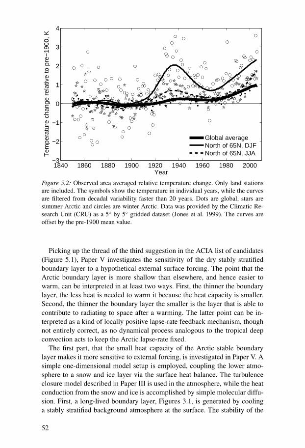
1840 1860 1880 1900 1920 1940 1960 1980 2000−3

−2

−1

0

1

2

3

4

Year

Tem

pera

ture

cha

nge

rela

tive

to p

re−

1900

, K

Global averageNorth of 65N, DJFNorth of 65N, JJA

Figure 5.2: Observed area averaged relative temperature change. Only land stationsare included. The symbols show the temperature in individual years, while the curvesare filtered from decadal variability faster than 20 years. Dots are global, stars aresummer Arctic and circles are winter Arctic. Data was provided by the Climatic Re-search Unit (CRU) as a 5◦ by 5◦ gridded dataset (Jones et al. 1999). The curves areoffset by the pre-1900 mean value.

Picking up the thread of the third suggestion in the ACIA list of candidates(Figure 5.1), Paper V investigates the sensitivity of the dry stably stratifiedboundary layer to a hypothetical external surface forcing. The point that theArctic boundary layer is more shallow than elsewhere, and hence easier towarm, can be interpreted in at least two ways. First, the thinner the boundarylayer, the less heat is needed to warm it because the heat capacity is smaller.Second, the thinner the boundary layer the smaller is the layer that is able tocontribute to radiating to space after a warming. The latter point can be in-terpreted as a kind of locally positive lapse-rate feedback mechanism, thoughnot entirely correct, as no dynamical process analogous to the tropical deepconvection acts to keep the Arctic lapse-rate fixed.

The first part, that the small heat capacity of the Arctic stable boundarylayer makes it more sensitive to external forcing, is investigated in Paper V. Asimple one-dimensional model setup is employed, coupling the lower atmo-sphere to a snow and ice layer via the surface heat balance. The turbulenceclosure model described in Paper III is used in the atmosphere, while the heatconduction from the snow and ice is accomplished by simple molecular diffu-sion. First, a long-lived boundary layer, Figures 3.1, is generated by coolinga stably stratified background atmosphere at the surface. The stability of the

52

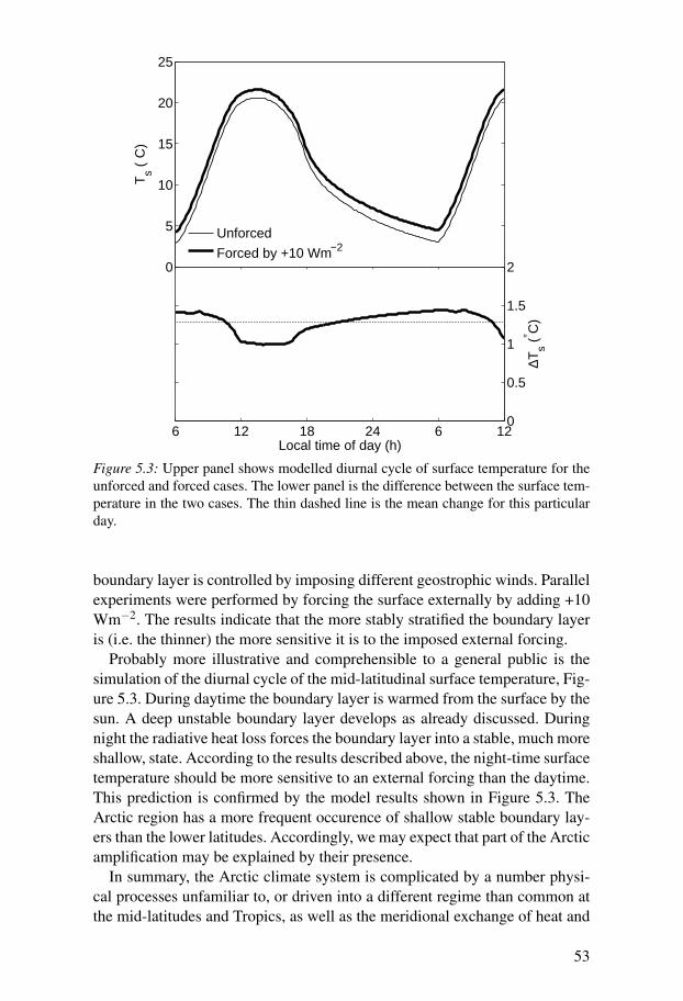
0

5

10

15

20

25

Ts (

° C)

Unforced

Forced by +10 Wm−2

6 12 18 24 6 120

0.5

1

1.5

2

Local time of day (h)

∆Ts (

° C)

Figure 5.3: Upper panel shows modelled diurnal cycle of surface temperature for theunforced and forced cases. The lower panel is the difference between the surface tem-perature in the two cases. The thin dashed line is the mean change for this particularday.

boundary layer is controlled by imposing different geostrophic winds. Parallelexperiments were performed by forcing the surface externally by adding +10Wm−2. The results indicate that the more stably stratified the boundary layeris (i.e. the thinner) the more sensitive it is to the imposed external forcing.

Probably more illustrative and comprehensible to a general public is thesimulation of the diurnal cycle of the mid-latitudinal surface temperature, Fig-ure 5.3. During daytime the boundary layer is warmed from the surface by thesun. A deep unstable boundary layer develops as already discussed. Duringnight the radiative heat loss forces the boundary layer into a stable, much moreshallow, state. According to the results described above, the night-time surfacetemperature should be more sensitive to an external forcing than the daytime.This prediction is confirmed by the model results shown in Figure 5.3. TheArctic region has a more frequent occurence of shallow stable boundary lay-ers than the lower latitudes. Accordingly, we may expect that part of the Arcticamplification may be explained by their presence.

In summary, the Arctic climate system is complicated by a number physi-cal processes unfamiliar to, or driven into a different regime than common atthe mid-latitudes and Tropics, as well as the meridional exchange of heat and

53

moisture with lower latitudes through atmospheric and oceanic transport. Aseries of mechanisms have been suggested as responsible for the Arctic am-plification, though the surface albedo feedback is most frequently quoted inthe literature. It is, however, being questioned if it is the driving mechanismor whether Arctic surface temperature change would be amplified even in itsabsence (Alexeev et al. 2005; Paper V).

54

6. Outlook

Understanding the Arctic climate system is one of the major problems facingclimate scientists of today. The widely quoted surface albedo climate feed-back mechanism blamed for Arctic amplification cannot explain the signatureof the observed warming. The warming is largest over land during the polarnight, when the surface albedo feedback is inactive. The debate on why theArctic is warming more rapidly than the rest of the globe is open. Several al-ternative explanations exist. Paper V contributes to the debate by suggestingthat the most extreme surface warming during winter over land could be dueto the shallow nature of the very stable boundary layer making it extra sensi-tive to external forcing. Future research should attempt to evaluate the relativeimportance of the many processes possibly contributing to Arctic amplifica-tion.

Observations presented in Paper II question the long-standing hypothesisthat turbulence should decay at large Richardson numbers. Turbulence underhighly stable conditions is, however, very different from turbulence at weakstability. It may not even qualify as being turbulence in the traditional sense.The only feature that really reveals its presence is the non-zero stress, τ . Inother words, a strongly stably-stratified flow will feel that an internal viscosityattempts to reduce the vertical shear. Further, the stress exerted by the turbu-lent motions serves to uphold the turbulence itself. Presently, we do not knowthe physical mechanism responsible for the presence of turbulence at strongstability. It would, however, not appear implausible that the turbulent motionat large Richardson numbers is somehow connected to internal gravity waves.

The exchange between the atmosphere, ocean and land surfaces actsthrough the boundary layer. This plays a key role in forecast and climatemodels for the representation of phenomena ranging from processes insoil, snow and ice, over the diurnal cycle and the development of cyclones,to the nature of the general circulation and the hydrological cycle. Someof the major biases present in models today can be attributed to the poorrepresentation of the boundary layer. Any improvements we wish to introducein these models, however, have to face the full range of phenomena thatdepend on the boundary layer.

There is a strong need for better communication between the scientificblocks of experimentalists, modelers and theoreticians, that are traditionwithin boundary-layer meteorology. An example is the improper modelinguse of Monin-Obukhov similarity, which was originally only intended for

55

near-neutral conditions. Nevertheless, modelers have extended it to bothvery convective and stably stratified conditions, possibly in the lack ofbetter? However, we have known for at least thirty years that observationaldata treated in this way suffer from self-correlation (Hicks 1978). Onemay speculate that this is part of the reason that leading forecast centershave abandoned Monin-Obukhov similarity for schemes that simply yieldsbetter forecasts for more-or-less unknown reasons. The ultimate test forthe turbulence closure model presented in Paper III will be in the plannedimplementation in weather forecasts and climate models.

56

Acknowledgements

Just as the arrival at the end of splendid journey, finishing my thesis brings outfeelings of both joy and a little bit of grief, knowing that it soon belongs to thepast. These last four and a half years of studies have been a great part of mylife, and I am deeply indepted to a large number of people and organisations.My fellow, friend and companion for most of the journey has been my super-visor Gunilla Svensson. With her firm hand she has guided me safely throughthe wild waters, at the same time providing me with the freedom to followmy heart and explore my curiosity. Sergej Zilitinkevich generously shared hisdeep theoretical wisdom, which serves as the foundation for much of the the-sis. Michael Tjernstöm sparked my interest in mesoscale meteorology and sci-ence in general, long before I started as graduate student. Later we had the op-portunity to further pursue our common curiosity. Branko Grisogono was thebest undergraduate teacher of mesoscale meteorology and he taught me almosteverything I know about it. The star that shines the brightest is Leif Enger, re-minding me of all the good things in life. In the end I owe the reason for beinghere to my beloved wife Malin. I thank Volodya Alexeev, Bob Beare, AntonBeljaars, Hans Bergström, Jenny Brandefeldt, Joan Cuxart, Peter Ditlevsen,Igor Esau, Rune Graversen, Nils Gustafsson, Bert Holtslag, Måns Håkansson,Johannes Karlsson, Nathan Kleorin, Erland Källen, Peter Langen, CarolineLeck, Gert Lenderink, Peter Lundberg, Jenny Lundén, Larry Mahrt, AnneMcCabe, Peter Minnett, Anders Moberg, Carmen Nappo, Jonas Nycander,Ola Persson, Igor Rogachevski, Ann-Sofi Smedmann, Gert-Jan Steeneveld,Johan Ström, Semion Sukoriansky, Stefan Söderberg, Dean Vickers, AndreasWickström, Mark Zagar, Nedjeljka Zagar and several others for inspiring, de-veloping and clarifying discussions and kind technical help invaluable to mywork. Financial support for my studies was from The Swedish Research Coun-cil. In addition, A. E. W. Smitts Scholarship Fund, The Knut och Alice Wal-lenberg Foundation and The Royal Swedish Research Academy of Sciencesprovided funding for many of the travels I have been fortunate to have made.Special thanks to The National Oceanic and Atmospheric Administration forhosting me for three months at their laboratories in Boulder, Colorado. They,and the American Meteorological Society, National Center for AtmosphericResearch, The GEWEX Atmospheric Boundary Layer Study, NATO, Interna-tional Arctic Reseach Center and The Norwegian Research Council arrangedmeetings, workshops, conferences, summerschools and provided the facilitiesinvaluable to the modern network of science.

57

References- Alexeev, V., P. Langen and J. Bates, 2005: Polar amplification of surface

warming on an aquaplanet in ghost forcing experiments without sea icefeedbacks. Climate Dyn. 24, 655–666.

- Anderson, T. L., R. J. Charlson, S. E. Schwartz, R. Knutti, O. Boucher, H.Rodhe and J. Heintzenberg, 2003: Climate forcing by aerosols – a hazypicture. Science, 300, 1103–1104.

- Arctic Climate Impact Assessment (ACIA), 2005. Cambridge UniversityPress, 1042 pp.

- Baas, P., G. J. Steeneveld, B. J. H. van de Wiel, and A. A. M. Holtslag,2006: Exploring self-correlation in flux-gradient relationships for stablystratified conditions. J. Atmos. Sci. 63, 3045–3054.

- Beare, R. J., J. Cuxart, A. A. M. Holtslag, I. Esau, J.-C. Golaz, M. A.Jimenez, M. Khairoutdinov, B. Kosovic, D. Lewellen, T. S. Lund, J. K.Lundquist, A. McCabe, M. K. MacVean, A. F. Moene, Y. Noh, S. Raaschand P. Sullivan, 2006: An intercomparison of large-eddy simulations of thestable boundary layer. Bound.-Layer Meteorol. 118, 247–272.

- Beljaars, A. C. M., 2001: Issues in boundary layer parametrization for largescale models. ECMWF seminar on: Key issues in the parametrization ofsubgrid physical processes, 71–88.

- Beljaars, A. C. M. and P. Viterbo, 1998: The role of the boundary layer in anumerical weather prediction model. In Clear and cloudy boundary layers,eds. A. A. M. Holtslag and P. G. Duynkerke. Royal Netherlands Academyof Arts and Sciences, 287–304.

- Bjerknes, J., and Solberg, H., 1922: Life cycle of cyclones and the polarfront theory of atmospheric circulation. Geophys. Publ. Norske Vidensk.-Akad. 3, 1–18.

- Blackadar, A. K. 1962: The vertical distribution of wind and turbulent ex-change in a neutral atmosphere. J. Geophys. Res., 67, 3095–3102.

- Bony, S., R. Colman, V. M. Kattsov, R. P. Allan, C. S. Bretherton, J.-L.Dufresne, A. Hall, S. Hallegate, M. A. Holland, W. Ingram, D. A. Ran-dall, B. J. Soden, G. Tselioudis and M. J. Webb 2006. How well do weunderstand and evaluate climate change feedback processes? J. Clim. 19,3445–3482.

- Cuxart J., A. A. M. Holtslag, R. Beare, A. Beljaars, A. Cheng, L. Conangla,M. Ek, F. Freedman, R. Hamdi, A. Kerstein, H. Kitagawa, G. Lenderik, D.Lewellen. J. Mailhot, T. Mauritsen, V. Perov, G. Schayes, G-J. Steeneveld,G. Svensson, P. Taylor, S. Wunsch, W. Weng and K-M. Xu, 2006: Single-column intercomparison for a stably stratified atmospheric boundary layer.Bound.-Layer Meteorol. 118, 273–303.

- Chandrasekar, S., 1961. Hydrodynamic and hydromagnetic stability, 103.Oxford University Press.

58

- Duynkerke, P. G., 1998: Dynamics of cloudy boundary layers. In Clear andcloudy boundary layers, eds. A. A. M. Holtslag and P. G. Duynkerke. RoyalNetherlands Academy of Arts and Sciences, 199–218.

- Ekman, V. W., 1902. Om jordrotationens inverkan på vindströmmar ihafvet. Nyt Magazin for Naturvidenskab. 40, 1–27.

- Fiedler, F. and H. A. Panofsky, 1970: Atmospheric scales and spectral gaps.Bull. Amer. Meteor. Soc. 51, 1114–1120.

- Frisch, U., 1995: Turbulence. Cambridge University Press, 296 pp.- Garratt, J. R., 1993: Sensitivity of climate simulations to land-surface and

atmospheric boundary-layer treatments – A review. J. Clim. 6, 419–448.- Garratt, J. R., P. B. Krummel, and E. A. Kowalczyk 1993: The surface

energy balance at local and regional scales – A comparison of general cir-culation model results with observations. J. Clim. 6, 1090–1109.

- Grachev, A. A., C. W. Fairall, P. O. G. Persson, E. L. Andreas and P. Guest,2005. Stable boundary-layer scaling regimes: The SHEBA data. Bound.-Layer Meteorol. 116, 201–235.

- Hansen, J., M. Sato and R. Ruedy, 1997: Radiative forcing and climateresponse. J. Geophys. Res., 102(D6), 6831–6864.

- Hicks, B. B., 1978: Some limitations of dimensional analysis and powerlaws. Bound.-Layer Meteorol. 14, 567–569.

- Holton, J. R. 2004: An introduction to dynamic meteorology. Elsevier Aca-demic Press, 535 pp.

- Houghton, J. T., Y. Dings, D. J. Griggs, M. Noguer, P. J. van der Linden,X. Dai, K. Maskell, C. A. Johnson, Eds., 2001: Climate Change 2001: Thescientific basis. Cambridge University Press, 944 pp.

- Howard, L. N., 1961. Note on a paper of John W. Miles. J. Fluid Mech., 10,509–512.

- Intieri, J. M., C. W. Fairall, M. D. Shupe, P. O. G. Persson, E. L. Andreas,P. S. Guest and R. E. Moritz, 2002: An annual cycle of Arctic surface cloudforcing at SHEBA. J. Geophys. Res., 107(C10), 8039.

- Jones, P. D., M. New, D. E. Parker, S. Martin and I. G. Rigor, 1999: Surfaceair temperature and its variations over the last 150 years. Rev. Geophys. 37,173–199.

- Kahl, J. D. W., D. A. Martinez and N. A. Zaitseva, 1996: Long-term vari-ability in the low-level inversion over the Arctic ocean. Int. J. Clim. 16,1297–1313.

- Klipp, C. L. and L. Mahrt, 2004. Flux gradient relationship, self-correlationand intermittency in the stable boundary layer. Quart. J. Roy. Meteor. Soc.,130, 2087–2103.

- Kolmogorov, A. N., 1941. On degeneration of isotropic turbulence in anincompressible viscous liquid. Dokl. Akad. Nauk SSSR 31, 538–540.

- Louis, J. F., 1979: A parametric model of vertical eddy fluxes in the atmo-sphere. Bound.-Layer Meteorol. 17, 187–202.

59

- Mahrt, L., J. Sun, W. Blumen, T. Delany and S. Oncley, 1998. NocturnalBoundary-Layer Regimes. Bound.-Layer Meteorol. 88, 255–278.

- Mahrt, L., 1999: Stratified atmospheric boundary layers. Bound.-Layer Me-teorol. 90, 375–396.

- Mahrt, L., and D. Vickers, 2003. Formulation of Turbulent Fluxes in theStable Boundary Layer. J. Atmos. Sci. 60, 2538–2548.

- Manabe, S., R. J. Stouffer, M. J. Spelman and K. Bryan, 1991: Transientresponses of a coupled ocean-atmosphere model to gradual changes of at-mospheric CO2. Part I: Annual mean response. J. Clim. 4, 785–818.

- Manabe, S., M. J. Spelman and R. J. Stouffer, 1992: Transient responsesof a coupled ocean-atmosphere model to gradual changes of atmosphericCO2. Part II: Seasonal responses. J. Clim. 5, 105–126.

- Mellor, G. L., and T. Yamada, 1974: Hierarchy of turbulence closure mod-els for planetary boundary layers. J. Atmos. Sci. 31, 1791–1806.

- Miles, J., 1961. On the stability of heteorogeneous shear flows. J. FluidMech. 10, 496–508.

- Miles, J., 1986. Richardson’s criterion for the stability of stratified shearflow. Phys. Fluids 29, 3470–3471.

- Monin, A. S., A. M. Obukhov, 1954: Basic laws of turbulent mixing in theground layer of the atmosphere. Akad. Nauk SSSR Geofiz. Inst. Tr., 151,163–187.

- Nastrom, G., K. Gage and W. H. Jasperson, 1984. Kinetic energy spectrumof large-and mesoscale atmospheric processes. Nature 310, 36–38.

- Nieuwstadt, F. T. M., 1984. The turbulent structure of the stable, nocturnalboundary layer. J. Atmos. Sci. 41, 2202–2216.

- Obukhov, A. M., 1946: Turbulence in an atmosphere with inhomogeneoustemperature. Tr. Inst. Teor. Geofiz. Akad. Nauk SSSR, 1, 95–115.

- Panofsky, H. A., and I. Van der Hoven, 1955: Spectra and cross spectra ofvelocity components in the mesometeorological range. Q. J. Roy. Meteorol.Soc. 81, 603–606.

- Persson, P. O. G., C. W. Fairall, E. L. Andreas, P. S. Guest and D. K. Per-ovich, 2002: Measurements near the atmospheric surface flux group towerat SHEBA: Near-surface conditions and surface energy budget. J. Geophy.Res. 107(C10), 8045.

- Pollard, R. T., P. B. Rhines and R. O. R. Y. Thompson, 1973: The deepeningof the wind-mixed layer. Geophys. Fluid Dyn. 3, 381–404.

- Popper, K. 1934: Logik der Forschung, Springer, Vienna.- Prandtl, L., 1929. Einfluss stabilisierender kräfte auf die turbulenz.

Vorträge aus dem Gebiete der Aerodynamik und verwandten Gebiete,pages 1–7, Springer.

- Randall, D. A. and B. A. Wielicki, 1997: Measurements, models, and hy-pothesis in the atmospheric sciences. Bull. Amer. Meteor. Soc.,78, 399–406.

- Richardson, L. F. 1920. The supply of energy from and to atmosphericeddies. Proc. R. Soc. A97, 354–373.

60

- Rossby, C.-G. and R. B. Montgomery, 1935: The layer of frictional influ-ence in wind and ocean currents. Papers in Physical Oceanography andMeteorology, 3(3). Massachusetts Institute of Technology and Woods HoleOceanographic Institution.

- Serreze, M. C. and J. A. Francis, 2006: The Arctic amplification debate.Clim. Change.,76, 241–264.

- Sorbjan, Z., 2006. Local structure of turbulence in stably-stratified bound-ary layers. J. Atmos. Sci., 63, 1526–1537.

- Steeneveld, G. J., B. J. H. van de Wiel and A. A. M. Holtslag, 2006a:Modeling the Arctic stable boundary layer and its coupling to the surface.Bound.-Layer Meteorol. 118, 357–378.

- Steeneveld, G. J., B. J. H. van de Wiel and A. A. M. Holtslag, 2006b:Modeling the evolution of the atmospheric boundary layer coupled to theland surface for three contrasting nights during CASES-99. J. Atmos. Sci.63, 920–935.

- Steeneveld, G. J., T. Mauritsen, E. I. F. de Bruijn, J. Vila Guerau de Arel-lano, G. Svensson, and A. A. M. Holtslag, 2007. Evaluation of the sta-ble boundary layer and diurnal cycle in the limited area models MM5,COAMPS and HIRLAM for three contrasting nights in CASES99. Sub-mitted to Journal of Applied Meteorology and Climate.

- Stull, R. B., 1988: An Introduction to Boundary Layer Meteorology. KluwerAcademic Publishers, 670 pp.

- Svensson, G. and A. A. M. Holtslag, 2007: Modelling the turning of windwith height in the stable boundary layer. Submitted to Quart. J. Roy. Mete-orol. Soc.

- Tjernström, M. 1993: Turbulence length scales in stably stratified free shearflow analyzed from slant aircraft profiles. J. Appl. Meteor., 32, 948–963.

- Tjernström, M., M. Zagar, G. Svensson, J. J. Cassano, S. Pfeifer, A. Rinke,K. Wyser, K. Dethloff, C. Jones, T. Semmler and M. Shaw 2005: Modellingthe Arctic boundary layer: An evaluation of six ARCMIP regional-scalemodels using data from the sheba project. Bound.-Layer Meteorol. 117,337–381.

- Thunis, P., and R. Bornstein, 1996: Hierachy of mesoscale flow assumptionand equations. J. Atmos. Sci. 53, 380–397.

- Vinnichenko, N. K. 1970: The kinetic energy spectrum in the free atmo-sphere - 1 second to 5 years. Tellus, 22, 158–166.

- Viterbo, P., Beljaars, A. C. M., Mahfouf, J.-F. and Teixeira, J., 1999: Therepresentation of soil moisture freezing and its impact on the stable bound-ary layer. Quart. J. Roy. Meteorol. Soc., 125, 2401–2426.

- Watanabe, O., J. Jouzel, S. Johnsen, F. Parrenin, H. Shoji and N. Yoshida,2003: Homogeneous climate variability across East Antarctica over the pastthress glacial cycles. Nature, 422, 509–512.

- Zilitinkevich, S. S., 1972: On the determination of the height of the Ekmanboundary layer. Bound.-Layer Meteorol. 3, 141–145.

61

- Zilitinkevich, S. S., 2002: Third-order transport due to internal waves andnon-local turbulence in the stably stratified surface layer. Quart. J. Roy.Meteor. Soc., 128, 913–925.

- Zilitinkevich, S. S., T. Elperin, N. Kleeorin, I. Rogachevskii, 2007: Energy-and flux-budget (EFB) turbulence closure model for stably stratified flows.Submitted to Bound.-Layer Meteorol.

- Zilitinkevich, S. S. and D. V. Mironov 1996: A multi-limit formulation forthe equilibrium depth of a stably stratified boundary layer. Bound.-LayerMeteorol. 81, 325–351.

62