Ocean Dynamics (2011) 61:1475–1490DOI 10.1007/s10236-011-0437-0

On the assessment of Argo float trajectory assimilationin the Mediterranean Forecasting System

Jenny A. U. Nilsson · Srdjan Dobricic ·Nadia Pinardi · Vincent Taillandier ·Pierre-Marie Poulain

Received: 27 October 2010 / Accepted: 9 May 2011 / Published online: 5 June 2011© The Author(s) 2011. This article is published with open access at Springerlink.com

Abstract The Mediterranean Forecasting System (MFS)has been operational for a decade, and is continuouslyproviding forecasts and analyses for the region. Theseforecasts comprise local- and basin-scale informationof the environmental state of the sea and can be usefulfor tracking oil spills and supporting search-and-rescuemissions. Data assimilation is a widely used methodto improve the forecast skill of operational modelsand, in this study, the three-dimensional variational(OceanVar) scheme has been extended to include Argofloat trajectories, with the objective of constraining andameliorating the numerical output primarily in termsof the intermediate velocity fields at 350 m depth.When adding new datasets, it is furthermore crucial to

Responsible Editor: Birgit Andrea Klein

J. A. U. Nilsson (B)National Institute of Geophysics and Vulcanology (INGV),Viale Aldo Moro 44, 6 floor, 40128 Bologna, Italye-mail: nilsson@bo.ingv.it

S. DobricicCentro EuroMediterraneo per i Cambiamenti Climatici(CMCC), Bologna, Italy

N. PinardiCorso di Scienze Ambientali, Bologna University,Ravenna, Italy

V. TaillandierLaboratoire d’Oceanographie de Villefranche(CNRS, UMPC), Villefranche-sur-Mer, France

P.-M. PoulainThe National Institute of Oceanography and AppliedGeophysics (OGS), Trieste, Italy

ensure that the extended OceanVar scheme does notdecrease the performance of the assimilation of otherobservations, e.g., sea-level anomalies, temperature,and salinity. Numerical experiments were undertakenfor a 3-year period (2005–2007), and it was concludedthat the Argo float trajectory assimilation improvesthe quality of the forecasted trajectories with ∼15%,thus, increasing the realism of the model. Furthermore,the MFS proved to maintain the forecast qualityof the sea-surface height and mass fields after theextended assimilation scheme had been introduced. Acomparison between the modeled velocity fields andindependent surface drifter observations suggestedthat assimilating trajectories at intermediate depthcould yield improved forecasts of the upper oceancurrents.

Keywords Ocean modeling · Data assimilation ·Argo floats

1 Introduction

A three-dimensional variational (3DVAR) assimila-tion scheme for Lagrangian trajectories was developedand tested by Taillandier et al. (2006b) and Taillandieret al. (2010) using Argo float surfacing positions duringa 3-month period in the North-Western MediterraneanSea. In these studies, encouraging results were obtainedalthough only four Argo floats were used in the nu-merical experiments. Here, a numerical study, takinginto account all Argo float surfacing positions availablein the Mediterranean Sea, has been undertaken fora 3-year period (2005–2007). The model results, with

1476 Ocean Dynamics (2011) 61:1475–1490

and without Argo float trajectory assimilation, wereassessed with special focus on the intermediate velocityfields at 350 m depth.

The numerical experiments have been performedusing the MFS, which has been in operational use for adecade and has continuously been providing forecastsand analyses for the region (Pinardi et al. 2003; Tonaniet al. 2008). These forecasts yield local- and basin-scale information of the state of the sea, e.g., sea level,velocity, temperature, and salinity fields, and can beuseful for search-and-rescue missions and for trackingoil spills (Coppini et al. 2010). For these purposes,it is crucial to provide state-of-the-art model output,and it has been established that OceanVar (Dobricicand Pinardi 2008) is capable of improving significantlythe overall quality of the MFS model fields (Dobricicet al. 2007). At present, the assimilated observationaldatasets are obtained from both remote sensing and insitu measurements, such as satellite-observed sea-levelanomalies (SLA, Le Traon et al. 2003), temperatureprofiles from expendable probes (XBT, Manzella et al.2007), as well as temperature and salinity profiles fromArgo floats (Poulain et al. 2007). In the present study,the Argo float positions obtained at the sea surface(Poulain et al. 2007; Menna and Poulain 2010) willbe added to this ensemble, with the primary aim ofconstraining and improving the modeled intermediatevelocity fields in the Mediterranean Sea.

The Mediterranean Sea is a deep semi-enclosedbasin connected to both the Atlantic Ocean and theBlack Sea through narrow straits. Its bathymetry ischaracterized by two major sub-basins, the Westernand Eastern Mediterranean, which are separated by ashallow sill (∼400 m) in the Sicily Channel, cf. Fig. 1.The thermohaline circulation is mainly driven by buoy-

ancy loss due to the evaporation as well as the lowprecipitation and fresh-water inflow in the area, thus,making the Mediterranean Sea one of the largest con-centration basin in the world. This inverse estuarinecirculation can be schematically described as a balancebetween the inflow from the Atlantic and the Levan-tine Intermediate Water (LIW) outflow (Benzohra andMillot 1970; Millot 1999). Most of the dense water isformed in the Gulf of Lions and the Levantine Basinsubduction zones, in particular, the LIW is formed inthe North-Eastern part of the Levantine Basin, where,due to buoyancy loss it sinks to its characteristic depthof ∼200–500 m depth. Thereafter, it spreads across theMediterranean through various pathways and finallyexits into the Atlantic Ocean through the Straits ofGibraltar, hereby closing the loop of what is knownas the Mediterranean conveyor belt, cf. Pinardi andMasetti (2000).

The Mediterranean circulation is, furthermore, char-acterized by well-defined coastal currents, such as theAlgerian Current (AC), as well as small-, meso-, andsub-basin-scale eddy structures in the interior of thebasin, cf. Millot (1991), Robinson et al. (1991). Mod-eling the meandering of these currents and calculatingthe evolution of the eddies is highly complex, thus thevelocity-field forecasts are often associated with largeuncertainties due to the inherent nonlinear dynamics ofthe circulation (cf. Molcard et al. 2002). In this context,assimilation of Lagrangian trajectories in operationalocean models could offer a possibility to reduce someof these errors and to ultimately yield more accurateocean forecasts.

The contents of the manuscript are disposed as fol-lows: Section 2 provides a general description of theMediterranean Forecasting System and the OceanVar

Fig. 1 Observed Argo floatpositions in theMediterranean Sea in2005–2007

Ocean Dynamics (2011) 61:1475–1490 1477

assimilation scheme, Section 3 describes the numeri-cal experiments, Section 4 subsequently presents anddiscusses the results, and finally Section 5 offers someconclusions.

2 The Mediterranean Forecasting System

The MFS consists of three fundamental constituents:the data collection network, the ocean general circu-lation model (OGCM), and the OceanVar assimila-tion scheme. The MFS daily cycle and its coupling isschematically illustrated in Fig. 2. Next, the Argo trajec-tory dataset will be presented, whereafter the completeforecasting system is described.

2.1 Argo float trajectories

Data from both Apex (manufactured by Webb Re-search Corporation, USA) and Provor (produced byNKE Electronics, France) profiling floats were pro-vided by the Coriolis Operational Oceanography datacenter and extensively quality checked by The Na-tional Institute of Oceanography and ExperimentalGeophysics (OGS) in Trieste. These floats, commonly

Fig. 2 Illustration of the MFS daily cycle and the coupling ofthe forcing (F), initial conditions (IC), the OGCM, OceanVar,and the observations (Obs). The OGCM produces 1-day fore-casts (background fields) and OceanVar calculates model fieldcorrections (analyses) daily

referred to as MedArgo floats, started to be deployedin the Mediterranean Sea in 2003 within the frameworkof the MFSTEP project. The MedArgo floats are pro-grammed to perform continuous cycles, in which thefloat descend from the sea surface to 350-m parkingdepth, where it drifts for a 4.5-day period. The cycleis completed by a 700-m dive (2,000 m every ten cy-cles), whereafter the float re-emerges to the sea surfaceand makes contact with the Argos satellite system andtransmits the data (e.g., surfacing coordinates, temper-ature, and salinity profiles). When the data-transferprocedure has been completed, after approximately 6 h,the float begins the next cycle by descending back tothe parking depth (cf. Menna and Poulain 2010). EachArgo float file holds information of time, float surfacingpositions as well as the corresponding water depth atthese locations. The depths were retrieved from theSmith and Sandwell Bathymetry (Smith and Sandwell1997) which is based on Satellite Altimeter data.

When Argo float coordinates are available, theOceanVar trajectory model computes 5-day trajectoryforecasts. Moreover, an algorithm in the daily assimi-lation cycle searches the observational time series forpertinent data on the “present day” (t = tf f=final) andon the “preceding Argo cycle day” (ti = tf -�t; i=initial,�t = 5 days), in order to perform trajectory data assim-ilation. In conjunction with this, the depths on these twooccasions were examined to preclude erroneous trajec-tory estimates when the float might have been stuckto the bottom. Problems of this type were avoided byconstraining the data selection so that only coordinatesobtained at locations with depths greater than or equalto 400 m were accepted (approximately 4% of the datawas rejected). The coverage of the Argo float positionsduring 2005–2007 is displayed schematically in Fig. 1,and the OceanVar trajectory model is presented furtherin Section 2.4.

2.2 The ocean general circulation model

The Océan Parallélise code (Madec et al. 1998) wasadapted to the Mediterranean Sea by Tonani et al.(2008) and served as OGCM in the numerical experi-ments. This model is based on the primitive equationssubjected to the Boussinesq and incompressibility ap-proximations, and thereafter, discretized on a sphericalgrid with a horizontal resolution of 1/16◦ × 1/16◦ (∼5–7 km depending on latitude). The model depths aredescribed by 72 unevenly spaced levels, with a 3-m layerthickness near the surface and 300 m near the bottom,hereby resolving the Mediterranean bathymetry in arealistic manner. The OGCM was spun up from astate of rest and forced by 1/2◦ horizontal resolution,

1478 Ocean Dynamics (2011) 61:1475–1490

6-h atmospheric fields from the European Centre forMedium-Range Weather Forecasts.

The water exchanges through the Gibraltar and Dar-danelles straits are dealt with in different manners, thelatter being implemented as a river (surface boundarycondition) with monthly inflow and salinity climatologyparameterizations (Adani et al. 2011; Kourafalou andBarbopoulos 2003). The open boundary in the Atlantic,on the other hand, is described by box (outer limitat 18◦ W) in which the flow across Gibraltar Straitis relaxed to climatology and vanishing currents areprescribed at the Atlantic model boundaries. The tem-perature and salinity along these borders are relaxedto Atlantic climatology at all depths. Moreover, theheat flux in the Mediterranean Sea is corrected byrelaxation of the modeled surface-layer temperatures(Dobricic et al. 2005) towards sea-surface temperatureobservations (SST, Marullo et al. 2007).

Due to the fact that Mediterranean basin is a con-centration basin, i.e., it has a net water loss since theevaporation exceeds the precipitation, the water bal-ance is defined to conserve mass under the conditionthat the net water flux at the sea surface is negative.The changes in the sea-surface salinity due to evap-oration and precipitation is, thus, modeled by relax-ation to the monthly MEDATLAS climatology values(MEDAR/MEDATLAS Group 2002), cf. Tonani et al.(2008).

2.3 The OceanVar assimilation scheme

The development of variational assimilation schemesfor atmospheric forecasting models started in the late1980s (Lorenc 1986), and research efforts since haveresulted in the highly advanced four-dimensional varia-tional schemes. The variational assimilation techniquesfor operational ocean forecasting purposes are not, atpresent, as sophisticated as the methods applied inoperational weather forecasting; however, continuousprogress is being made in this field (cf. Dobricic 2009).Implementation of 3DVAR assimilation schemes inocean models is not straight forward, due to the vari-able model-domain lateral boundaries (coast lines) andbathymetry and to overcome these challenges newpractical solutions have had to be found (cf. Dobricicand Pinardi 2008).

Although the amount of oceanic observations isquite modest compared with those available for theatmosphere, the assimilation of these somewhat limiteddatasets was found to yield more accurate ocean fore-casts (Dobricic et al. 2007). In this context, it shouldbe mentioned that the computational cost related tothe 3DVAR assimilation procedures is less dependent

on the number of observations, but mostly on the sizeof the model state vector, (i.e., the number of modeloutput variables). This implies that the CPU time willnot be significantly affected if, at a later stage, furtherobservational datasets were to be added to the forecast-ing system.

In this numerical study, OceanVar has been ex-tended to also assimilate Argo float positions us-ing a trajectory model as the observational operator(Taillandier and Griffa 2006; Taillandier et al. 2010).Hereby, Argo float trajectories are being added to thewide range of variables that are already being assimi-lated operationally, e.g., SLA and in situ observationsof temperature and salinity profiles from Argo floatsand temperature profiles from XBTs.

The OceanVar minimizes by iterations a cost func-tion formulated as:

J = 1

2(x − xb )T B−1 (x − xb )

+1

2(H(x) − y)TR−1(H(x) − y). (1)

Here, x is the model state vector, xb the backgroundstate vector, y the observational vector, B the back-ground error covariance matrix, R the observational-error covariance matrix, H the nonlinear observationaloperator, and T denotes the vector transpose (e.g.Lorenc 1997). The model state vector contains the tem-perature, salinity, velocity, and sea-level model outputin matrix form as x = [T S U V η]T .

In order to set-up the minimization routine, aquadratic cost function is created by linearizing Eq. 1around the background state vector xb , yielding:

J = 1

2δxTB−1δx + 1

2(H(δx) − d)TR−1(H(δx) − d), (2)

where δx = x − xb are the increments and H is thelinearized observational operator. The so-called misfits(the differences between the observations and thebackground fields) are contained in d = [y − H(xb)],where the nonlinear operational operator, H, transfersthe model variables onto the observational grid, herebyallowing direct comparisons between the two datasets.J is rapidly minimized in iterations, in which it is neces-sary to calculate J and its gradient ∇ J. The calculationof ∇ J requires the application of adjoint operators foreach linear operator appearing in J.

In OceanVar, the increments are written in terms ofthe control vector v and the matrix V:

δx = Vv, (3)

Ocean Dynamics (2011) 61:1475–1490 1479

where V is constructed as B = VVT . Thus, the lin-earized cost function J can be reformulated for thetransformed space as:

J = 1

2vTv + 1

2(HVv − d)TR−1(HVv − d). (4)

The background error covariance matrix, B, is mod-eled as a sequence of linear operators (cf. Dobricic andPinardi 2008) as:

V = VDVuvVηVHVV, (5)

where VV contains multi-variate temperature (T) andsalinity (S) Empirically Orthogonal Functions (EOFs)computed from model output. The EOFs include infor-mation on both the temporal and the spatial variabilityin the Mediterranean; the year is divided in four sea-sons, and the basin into 13 regions due to the largedifferences in seasonal and local dynamics (Demirovet al. 2003; Dobricic et al. 2005). VH applies Gaussian-distributed horizontal covariances with constant cor-relation radii on the vertical T and S fields, herebyyielding three-dimensional spatial covariances as VS =VHVV . Sea-surface height (SSH) error covariances areprovided by Vη based on the T and S corrections anda barotropic linear model explained by Dobricic andPinardi (2008). Vuv calculates the baroclinic compo-nents of the velocity correction in geostrophic balancewith the surface pressure gradient, and VD applies adivergence damping filter on the velocity field.

The corrections of the velocity fields due to trajec-tory assimilation enter in the Vuv operator, and canthereafter influence the sea level through Vη, and thefull 3D mass fields through VS. The observational-error covariance matrix, R, contains information of theobservational errors, and hence sets the weight (relatedto the data reliability and representativity) in the cor-rections of the model state estimate.

In conclusion, in each iteration OceanVar perturbsthe coefficients that are multiplied with the verticalEOFs. By the application of linear operators, those per-turbations are transformed into velocity perturbations,which thereafter are used as input for the linearizedtrajectory model represented by the observational op-erator H. Furthermore, the integration of the lineartrajectory model yields perturbations of the last Argofloat position HVv that can be subtracted from themisfit d. The linearized trajectory model representedby H in Eqs. 2 and 4, as well as the computations ofpredicted and analyzed float positions will be describednext.

2.4 The OceanVar trajectory model

A trajectory model was implemented in the nonlinearobservational operator, thus providing a possibility tocorrect the modeled velocity fields by the observedArgo surfacing coordinates. The forecasted trajectorieswere calculated from the Eulerian model velocity fieldsby 5-day integrations of the particle advection equation(Eq. 6), starting on the latest observed float positions.The advection equation states that the fluid velocity ina fix point (in space and time) is equal to the velocityof a fluid parcel that is located in that position at thattime; this relation is described by the nonlinear first-order differential equation:

drdt

= uL(r(t), t). (6)

where r is the float position, and uL represents the La-grangian velocities at the float parking depth during thedrift period. The Eulerian velocities u can be describedin the Lagrangian framework as uL(r(t), t) =L(r(t))u(t),where L is the bilinear Lagrange interpolator. Thetime-integrated advection equation yields the fully non-linear trajectory model H(u), to be discretized andimplemented in the nonlinear observational operatorH for OceanVar, and is here presented for one step ofintegration:

r(tf ) = r(ti) +∫ tf

tiL(r(t))u(t)dt, (7)

where ti and tf = ti + �t indicates the limits of timeinterval (here, �t = 5 days). However, the nonlinearityof this equation imposes a severe analytical problemwhen the background velocity fields at the observa-tional positions are to be retrieved. Hence, a tangent-linear approximation was applied to Eq. 7 as proposedby Taillandier et al. (2006a), thus yielding the lin-earized perturbation equation, which will provide thelinearized observational operator H with the Eulerianvelocity increments δu:

δr(tf ) = δr(ti) +∫ tf

ti

(∂uL

∂u

∣∣∣∣r=rb

δu + ∂uL

∂r

∣∣∣∣u=ub

δr

)dt.

(8)

where the position and the Eulerian velocity incre-ments (δr = r − rb and δu = u − ub) are evaluatedaround the background velocity ub and backgroundposition rb . Moreover, transforming the Lagrangianvelocities (uL) to Eulerian (u), the partial derivativesin Eq. 8 can be rewritten as ∂uL

∂u =L(rb ), and ∂uL∂r =

L · u(rb ), where L is the derivative of L around the

1480 Ocean Dynamics (2011) 61:1475–1490

background position rb at the time tb . The equal-ity of Eq. 8 is assumed to be fulfilled when thehigher-order (nonlinear) terms in Eq. 7 are negligible(O(δr2, δu2) ∼0). This equation was given in discretizedform by Taillandier et al. (2006a) in Eq. 2.

In summary, 5-day trajectory predictions are com-puted for each Argo float from the model velocity fieldsby the nonlinear trajectory model Eq. 7, starting at theirrespective surfacing positions. When a float has fulfilledan “Argo cycle,” the OceanVar computes the analyzedfloat position and the analyzed trajectory, a procedurewhich requires the present and prior float coordinates.The analyzed position is obtained by minimizing thedistance between the present observed float positionand the “background position,” i.e., the last position ofthe “float” trajectory produced by a 5 days long integra-tion of the trajectory model, in the cost function (Eq. 2)through the linear operator H(δu). From this analyzedposition, the adjoint operator thereafter recalculatesthe trajectories between the analyzed positions and theprior observed positions.

Fig. 3 Schematic figure of observed and modeled trajectoriesstarting from an observed float position at t = ti. The precision ofthe MFS velocity fields is evaluated from the differences betweenthe observed float (obs) and the predicted (CTRL and TRAJfcst) as well as the analyzed (TRAJ an) float positions at t =ti + �t, where �t = 5 days

The OceanVar assimilates data in a daily cycle whiletrajectories are 5 days long. This inconsistency is ne-glected by assuming that the innovation is constantthroughout the trajectory integration time. That is, inEq. 8, the background velocity fields are stored duringthe 5 days long period with the temporal frequencyof 6 h, but it is assumed that δu (Eulerian) does notchange with time. After OceanVar has finished its dailyroutine, the initial float position for the next Argo cycleis re-set with the observed Argo float position, r(ti) =robs(ti), i.e., the initial float position are held fixed in theOceanVar (δr(ti) = 0), and only the final positions areperturbed by Eq. 8.

Comparisons between the trajectory predictionsfrom numerical experiments (with and without trajec-tory assimilation) and the observed Argo float posi-tions allows an evaluation of the consistency of thevelocity field corrections. The impact of the correc-tions of the velocity fields can furthermore be assessedquantitatively by calculating the distance between theend points of the trajectories produced at an arbitraryt = ti and the corresponding observed float positionsat tf =ti + �t. A schematic figure of the predicted andanalyzed trajectories at parking depth during one Argocycle is provided in Fig. 3.

3 The numerical experiments

3.1 Experimental model setup

Two numerical experiments (cf. Table 1) were under-taken in order to evaluate the impact of the assimilationof Argo float trajectories on the model state variables.Both experiments run the OGCM daily and produce24-h mean three-dimensional temperature, salinity, andvelocity fields, as well as two-dimensional SSH fields.These fields are typically denoted model backgroundfields (Daley 1991), and in this case they are actually 1-day forecasts. After the computation of the backgroundfields, OceanVar assimilates the “present-day” obser-vations and the model analysis is calculated, cf. Fig. 2.

Table 1 Design of the numerical experiments

EXP SLA T S TRA

CTRL X X XTRAJ X X X X

The assimilated observations are marked with XSLA sea-level anomalies, T temperature profiles, S salinityprofiles, TRA Argo float positions

Ocean Dynamics (2011) 61:1475–1490 1481

Both the control (CTRL) and trajectory assimila-tion (TRAJ) experiments assimilate on a daily basissatellite-measured SLA and SST as well as in-situ ob-servations of temperature and salinity, moreover, inthe TRAJ experiment are also Argo float positionsassimilated. In the case when no observations wereavailable, no corrections were calculated and the nextdaily MFS cycle was initialized.

3.2 Model-result evaluation

Comparisons of the CTRL and TRAJ daily forecasts,as well as their corresponding analyses can give anindication of where and how the model fields havebeen corrected by OceanVar. The differences in theCTRL and TRAJ background fields are due to thedifferent daily initial conditions, since the assimilatedobservational datasets are not identical, cf. Table 1 andFig. 2. Hence, by studying the discrepancies betweentheir respective background fields, the impact of thepreviously assimilated Argo trajectories on the modelfields as well as the propagation of the velocity fieldcorrections can be evaluated.

The quality of the model fields is assessed by com-parisons with observed datasets, and the differencesbetween the background fields and the observationsare known as “misfits.” In this study, the misfits havebeen calculated daily from the OGCM output usingthe “present-day” SLA, temperature, salinity and Argofloat positions, and since the daily assimilation pro-cedure has not yet been performed this comparisoncan be regarded as independent. In the next step, theobservations are assimilated by OceanVar, whereafterthe analysis is compared with the same observations. Inthis case, the comparison is not independent, but thedifferences between the analyses and the observationsare still interesting as they provide a measure of howthe model fields have converged towards the observedstate of the ocean.

3.3 Observational error sensitivity study

Before starting the numerical study, a year-long (2005)sensitivity test focusing on the observational positionerror for the Argo floats was carried out. The obser-vational float position error was first set a horizontaldistance of 500 m, based on the inherent Argos doppler-based positioning errors (∼250–1,500 m, cf. Menna andPoulain 2010) of the measurements. Root mean square(RMS) float position misfits were calculated and aver-aged over the test period and the Mediterranean, andthe preliminary results indicated that adding trajectoryassimilation makes the intermediate-current forecasts

more accurate (CTRL, 30 km and TRAJ500 m: 25.6 km).However, the OceanVar scheme experienced conver-gence problems due to the “small” observational error,and it was found that a 2, 000-m observational errormade the iteration procedure in OceanVar more stableand yielded slightly better estimates of the modeledtrajectories (TRAJ2,000 m: 24.4 km).

4 Results

4.1 Statistical analysis

4.1.1 The modeled f loat positions

The results from the sensitivity study suggested generalimprovements of the MFS float position forecastingskill. This was corroborated by the results from a moreextensive statistical study on the differences betweenthe modeled and observed float trajectories for theentire 3-year period in the Mediterranean Sea.

RMS float position misfits were calculated betweenthe observations and the CTRL and TRAJ output,and these diagnostics were thereafter averaged over2-week intervals (∼3 float cycles) in order to assurereliable statistics for the Mediterranean Sea. The resultspresented in Fig. 4 indicate that the use of OceanVartrajectory assimilation yield more accurate velocity

Fig. 4 Two-week Mediterranean mean float position RMSmisfits from the CTRL (black) and the TRAJ (red) experiments,as well as RMS differences in float positions between the TRAJanalyses and the observations (green)

1482 Ocean Dynamics (2011) 61:1475–1490

field forecasts at intermediate depth in the Mediter-ranean. This improvement was quantified in terms ofrelative differences (%) between the 3-year averagesof the CTRL and TRAJ RMS float position misfits (28and 23.6 km, respectively) and found to be around 15%.Moreover, RMS differences were calculated betweenthe TRAJ analyses and the observed float positions,and it was found that the quality of the trajectoryanalyses is on the order of the model horizontal gridresolution (∼5–7 km). The statistics were based on afairly homogenous supply of trajectory observations(approximately two communicating floats per day),with a total number of 795, 822, and 682 Argo cyclesin the years 2005, 2006, and 2007, respectively.

These results ultimately confirm that the trajectorymodel was implemented in a satisfactory manner intothe OceanVar routines.

4.1.2 The sea level and mass f ields

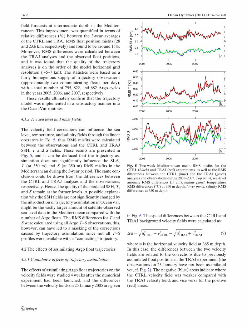
The velocity field corrections can influence the sealevel, temperature, and salinity fields through the linearoperators in Eq. 5, thus RMS misfits were calculatedbetween the observations and the CTRL and TRAJSSH, T and S fields. These results are presented inFig. 5, and it can be deduced that the trajectory as-similation does not significantly influence the SLA,T (at 350 m) and S (at 350 m) RMS misfits in theMediterranean during the 3-year period. The same con-clusion could be drawn from the differences betweenthe CTRL and TRAJ analyses and the observations,respectively. Hence, the quality of the modeled SSH, T,and S remain at the former levels. A possible explana-tion why the SSH fields are not significantly changed bythe introduction of trajectory assimilation in OceanVar,might be the vastly larger amount of satellite-observedsea-level data in the Mediterranean compared with thenumber of Argo floats. The RMS differences for T andS were calculated using all Argo T–S observations, this,however, can have led to a masking of the correctionscaused by trajectory assimilation, since not all T–Sprofiles were available with a “connecting” trajectory.

4.2 The effects of assimilating Argo float trajectories

4.2.1 Cumulative ef fects of trajectory assimilation

The effects of assimilating Argo float trajectories on thevelocity fields were studied 4 weeks after the numericalexperiment had been launched, and the differencesbetween the velocity fields on 25 January 2005 are given

a

b

c

Fig. 5 Two-week Mediterranean mean RMS misfits for theCTRL (black) and TRAJ (red) experiments, as well as the RMSdifferences between the CTRL (blue) and the TRAJ (green)analyses and observations during 2005–2007. Top panel, sea-levelanomaly RMS differences (in cm); middle panel, temperatureRMS differences (◦C) at 350 m depth; lower panel, salinity RMSdifferences at 350 m depth

in Fig. 6. The speed differences between the CTRL andTRAJ background velocity fields were calculated as:

�u =√

u2CTRL + v2

CTRL −√

u2TRAJ + v2

TRAJ, (9)

where u is the horizontal velocity field at 365 m depth.In this case, the differences between the two velocityfields are related to the corrections due to previouslyassimilated float positions in the TRAJ experiment (theobservations on 25 January have not been assimilatedyet, cf. Fig. 2). The negative (blue) areas indicate wherethe CTRL velocity field was weaker compared withthe TRAJ velocity field, and vice versa for the positive(red) areas.

Ocean Dynamics (2011) 61:1475–1490 1483

Fig. 6 An example ofpropagation of velocitycorrections (in cm−1) in themodel fields, here shown as:a speed differences betweenthe CTRL and TRAJbackground fields on 25January 2005 and b speeddifferences between theCTRL and TRAJbackground fields from the25 to the 26 of January.Theblack dots mark in (a) thepositions of all previouslyassimilated Argo floats and in(b) the Argo float positionsassimilated on 25 January

a

b

The largest velocity differences (generally around ±3 cm−1) were found in the vicinity of previously assim-ilated Argo floats (1–24 January), cf. the black dots inFig. 6a. However, in many of these regions trajectorydata had not been assimilated for several days, whichindicates that the corrections made by OceanVar re-main in the modeled velocity field memory at least onthe order of the “Argo cycle” (�t).

On January 25, surfacing coordinates from Argofloats were obtained in the AC (float 50769) andoff the Spanish North-East coast (float 35504) asshown by the black dots in Fig. 6b. These positionswere subsequently assimilated by OceanVar and inorder to evaluate the impact of trajectory assimila-tion from one day to another, the speed differencesbetween the CTRL and TRAJ background velocity

fields on 25–26 January were calculated as detailedbelow:

�u =√

[uCTRL(26)−uCTRL(25)]2+[vCTRL(26) − vCTRL(25)]2

−√

[uTRAJ(26)−uTRAJ(25)]2+[vTRAJ(26)−vTRAJ(25)]2.

(10)

The largest changes in the velocity fields in Fig. 6bwere found close to the two assimilated Argo floats,however, less evident alterations were found in most ar-eas where trajectories had previously been assimilated.These findings further corroborate the assumption thatvelocity field corrections from previous assimilation

1484 Ocean Dynamics (2011) 61:1475–1490

cycles propagate both in time (on the order of ∼�t) andacross the model domain.

4.2.2 Local impact on the modeled velocity f ields

The statistical analysis of the modeled trajectories gaveat hand that the trajectory assimilation make the fore-casted intermediate velocity fields more accurate. Here,the representativity of the modeled trajectories duringthe float drift at parking depth are to be examined.Observed float positions were compared with theCTRL- and TRAJ-modeled trajectories, and theircorresponding velocity fields. Figure 7 offers an ex-ample of these comparisons for Argo float (50769)that was observed off the Algerian coast in January2005. The CTRL and TRAJ trajectory predictions ofthe float drift, made on 20 January, were added toFig. 7a, b.

Moreover, the TRAJ velocity background field on 26January is provided in Fig. 7c, this to be interpreted asthe “analyzed” fields for the previous day, since initial

conditions had been corrected by the 25th Januaryobservations (cf. Fig. 2). The analyzed trajectory on25 January has been superimposed on the “analyzed”velocity field.

The well-developed (but erroneous) eddy at approx-imately 2◦40′ E, 37◦40′ N, that causes the northward di-rection of the predicted trajectory in the CTRL velocityfields, is somewhat reduced in the TRAJ backgroundvelocity fields. However, both predicted trajectories(made on 20 January) failed to arrive to the observedfloat position on 25 January. This is probably address-able to the high day-to-day variability of the meander-ing AC system which may be responsible of a decreasein the reliability of the 5-day trajectory forecasts in thisarea.

The direction and strength of the “analyzed” velocityfield is representative of the analyzed trajectory, and ingood agreement with the observed float positions. Inthis case, these results suggest that trajectory assimila-tion can improve the quality of the modeled velocityfields both in terms of forecasts and analyses.

Fig. 7 Zoom in on theAlgerian current velocityfields (in cm−1) at 365 mdepth: a the CTRLbackground fields on25 January, b the TRAJbackground fields on 25January, and c the TRAJbackground fields on 26January. The observed“50769 float” positions on 10,15, 20, and 25 January aremarked as black (notassimilated) and red(assimilated) dots; the firstposition is indicated with alarger marker. The predicted“50769 float” trajectorieswere marked with red thicklines in (a) and (b). Theanalyzed “50769 float”trajectory was added in (c)

a b

c

Ocean Dynamics (2011) 61:1475–1490 1485

Fig. 8 Meridional transect ofthe Algerian Current(3◦23′ E) showing the verticalpropagation of correctionsdue to trajectory assimilationon 25 January 2005: a theCTRL zonal velocity fields(in cm−1), b the TRAJ zonalvelocity fields (in cm−1), andc the differences between theCTRL and TRAJ zonalvelocity fields. The black dotsindicate the position of the“50769 float” before surfacingon 25 January

a b

c

Fig. 9 Meridional transect ofthe Algerian Current(3◦23′ E) showing the verticalpropagation of correctionsdue to trajectory assimilationon 25 January 2005: a theCTRL temperature fields(◦C), b the TRAJtemperature fields (◦C), andc the differences between theCTRL and TRAJtemperature fields. The blackdots indicate the position ofthe “50769 float” beforesurfacing on 25 January

a b

c

1486 Ocean Dynamics (2011) 61:1475–1490

4.2.3 Vertical propagation of corrections

The temperature and salinity RMS misfits at interme-diate depth in Fig. 5b, c showed no significant influenceof the trajectory assimilation, however, changes in theT and S vertical distributions due to the altered velocityfields are likely to occur.

This plausible vertical propagation of OceanVar cor-rections in the velocity and mass fields is here exam-ined in the framework of float 50769 in the AC. TheCTRL and TRAJ zonal velocity fields as well as thedifferences between them along 3◦23′ E are given inFig. 8 on 25 January 2005. The black dots indicate theposition of the float before surfacing on 25 January. Itwas noted that the largest differences in the velocityfields were found in the upper 300 m. Moreover, thepositioning of the AC core was shifted ∼0.1◦ northand the westward surface flow around 37◦30′–38◦ Nwas weaker in the TRAJ fields (2–6 cm−1). This factis further illustrated in Fig. 7b, where the small gyre at3◦40′ E, 37◦ N in the TRAJ fields forces a northwardmeandering of the AC.

Similar conclusions could be drawn for the massfields along this transect. The most important discrep-ancies in the T fields (cf. Fig. 9) were related to the shiftof the AC and found in the upper 300 m of the water

column. The changes of the temperature gradients dueto trajectory assimilation yielded T differences on theorder of 0.2◦C in the coastal area. The core of slightlywarmer water (�T ∼0.05◦C at 400 m, probably of LIWorigin) compared with the surrounding water mass atapproximately 200–500 m depth, was to a large extentreduced in the TRAJ fields.

The transect of the salinity distribution in Fig. 10suggested changes in the upper 200 m due to the shiftof the meandering AC, and the largest differences werefound in the coastal region where the TRAJ fieldswere generally fresher (�S∼0.04–0.1) than the CTRLoutput. In this case, the trajectory assimilation tendedto make the coastal current both colder and fresher,hence changing its buoyancy properties. Next, the accu-racy of the alterations in the vertical is to be evaluatedby comparing the in situ T–S profile from Argo float50769 with the corresponding CTRL and TRAJ modelprofiles.

The RMS misfits and the RMS differences betweenthe analyses and the observed profile were calculatedfor both model outputs on 25 January. To establishif trajectory assimilation has a long-term influence onthe vertical T and S structure, these diagnostics werealso calculated as 3-year mean values using all availablefloat profiles. The results are presented in Fig. 11,

Fig. 10 Meridional transectof the Algerian Current(3◦23′ E) showing the verticalpropagation of correctionsdue to trajectory assimilationon 25 January 2005: a theCTRL salinity fields, b theTRAJ salinity fields, andc the differences between theCTRL and TRAJ salinityfields. The black dots indicatethe position of the “50769float” before surfacing on25 January

a b

c

Ocean Dynamics (2011) 61:1475–1490 1487

and it was found that trajectory assimilation appearto not have a significant influence on the T and Sanalyses on either synoptic or longer time scales. Thisstatement holds true also for the 3-year mean T and SRMS misfits, however, the corresponding values basedon the 25 January fields showed notable discrepanciesbetween the CTRL and TRAJ outputs in the upper350 m of the water column.

It can be deduced from Fig. 11a, b that, on thisoccasion, the TRAJ experiment yields locally less ac-curate temperature and salinity background fields thanCTRL. The TRAJ temperature and salinity provedto be approximately 0.01–0.02◦C and ∼0.08 units lessaccurate in the upper 300 m, respectively, compared

with the CTRL results. Although, as the temperatureobservational error is ∼0.01◦C, it is noteworthy thatthe representativity of the temperature observation isat its limit. The salinity observational error is ∼0.01units which implies that in this case, the trajectoryassimilation has introduced errors locally in the salinityfields.

These overall results indicate that the assimilationof Argo trajectories not only affects the intermediatecurrents, but can indeed change the local properties ofthe state variables above parking depth. For example,a local change of ±6 cm−1 in the zonal velocity fieldscorresponds to an increase/decrease in transport ofapproximately 0.13 Sv for a current cross-section area

Fig. 11 Vertical profiles ofRMS differences betweenmodel values andobservations. Upper panelsshow snapshots from float50769 on 25 January 2005 ofthe a temperature andb salinity in the AlgerianCurrent. Lower panels show3-year mean c temperatureand d salinity estimates in theMediterranean Sea. The linesare color coded as follows:CTRL misfits (black), TRAJmisfits (red), CTRLanalyses-observationsresiduals (blue), and TRAJanalyses-observationsresiduals (green)

a b

c d

1488 Ocean Dynamics (2011) 61:1475–1490

of 100 m depth and ∼0.2◦ in width, hence on the orderof 10% of the net transport in the Algerian current (1.7Sv according to Benzohra and Millot 1970).

4.3 Independent comparisons with surface driftertrajectories

Daily observations of surface drifter positions (lowpassfiltered with a cut-off frequency of 36 h) were madeavailable by OGS through the Mediterranean SurfaceVelocity Programme (MedSVP) for validation of themodel velocity fields. The surface buoy of the drifteris attached to a drogue which is centered at 15 m depth(cf. Gerin et al. 2009) hereby making the observationsrepresentative of the near-surface circulation.

During 2006, a large number of Argo floats werelocated in the Eastern Mediterranean, and in particularwithin the Levantine basin. It was noted that Argofloat 50761 was drifting in the Mersa–Matruh gyre inDecember 2006 and, at this moment, surface drifter

59770 was located in the proximity of this gyre at adistance of approximately 50 km from the float. Hence,an opportunity was found to assess the influence of(Argo float) trajectory assimilation on meso-scale gyresystems and the accuracy of the surface velocity fields.

The CTRL and TRAJ velocity fields at 15 and 365 mdepth are provided in Fig. 12 on 16 December 2006. TheArgo float positions on 1, 6, 11, and 16 December aremarked with black (not assimilated) and red (assimi-lated) dots, while the surface drifter positions during16–21 December are marked with black stars. TheCTRL and TRAJ predicted float trajectories during11–16 December were added in red to their correspond-ing 365-m velocity fields in the lower panels. Further-more, the analyzed float trajectory was superimposedon the TRAJ 365-m velocity field in black.

The Mersa–Matruh gyre, located at 28◦30′–29◦30′ Eand 33–34◦ N, is one of the strongest sub-basin scalefeatures in the Eastern Mediterranean (Golnaraghi1993; Taupier-Letage 2008), here showing typical upper

Fig. 12 Validation of TRAJvelocity fields usingindependent surface drifterdata in the Levantine on 16December 2006. Top panelsshow velocity fields (in cm−1)at 15 m depth deduced fromthe a CTRL and b TRAJexperiments. The lowerpanels present the velocityfields at 365 m depth: c CTRLwith forecasted “50761 float”trajectory marked in red andd TRAJ with thecorresponding predicted(red) and analyzed (black)“50761 float” trajectories.The observed “50761 float”positions (1–16 December)are marked with black (notassimilated) and red(assimilated) dots. Thesurface drifter (59770)positions on 16–21 Decemberare marked with black stars.The first float and drifterpositions are indicated withlarger markers

a b

c d

Ocean Dynamics (2011) 61:1475–1490 1489

thermocline velocities on the order of 30 cms−1. Thestructure and strength of the gyre varies between theCTRL and TRAJ velocity fields (cf. Fig. 12c and d),although its horizontal dimensions of 1◦×1◦ are roughlymaintained. Both the CTRL and TRAJ float trajectorypredictions underestimated the gyre velocity, while theanalyzed trajectory was capable of reproducing theobserved float position on 16 December.

The corrections of the intermediate velocity fieldsproved to propagate vertically towards the surface lay-ers in the TRAJ experiment, this due to the barotropiclinear model in Vη (cf. Eq. 5). Moreover, these cor-rections altered the structure and the strength of thegyre at 15 m depth, and reduced the eddy meanderingnear 29◦45′ and 34◦ N, cf. Fig. 12a, b. In this case,the velocity field corrections appear to have improvedthe representation of the upper 400 m velocity fields.During this period, the CTRL experiment forecasted adistinct northward flow around 30◦16′E, 34◦30′ N whilethe TRAJ results suggested a somewhat weaker north-eastward flow (shown only for 16 December).

The observed drifter positions on 16–21 Decemberindicated that the TRAJ velocity fields were in betteragreement with the true state of the ocean on thisoccasion. Ultimately, this example shows that trajectoryassimilation can in some cases improve the forecastquality of the velocity fields above the Argo float park-ing depth.

5 Conclusions

Basin-wide trajectory assimilation experiments havebeen undertaken for a 3-year period (2005–2007) inthe Mediterranean Sea. It has been established thatthe extended OceanVar assimilation scheme is capableof improving the quality of the intermediate velocityfields based upon analyses. Indeed, statistical studies ofthe root mean square differences between the observedand forecasted float positions showed that ∼15% moreaccurate velocity fields are obtained when trajectoryassimilation was performed. The accuracy of the trajec-tory analyses was found to be on the order of the modelhorizontal grid resolution.

Furthermore, it was demonstrated that OceanVarmanages to minimize the differences between the ve-locity fields and the Argo float positions, this withoutintroducing spurious values in the modeled velocity,sea-surface height and mass fields. Occasionally, thevelocity field corrections caused local degeneration (inthe upper 300 m) of the temperature and salinity qualityon the order of the observational error. This problemwas probably caused by an inaccurate representation of

the local T and S error variability in the EOF-basedcovariance error matrix. However, this inconsistencyproved to be statistically insignificant as the 3-yearmean RMS misfit profiles indicated no negative impacton the vertical mass structure in the Mediterranean Seain general.

MFS proved capable of yielding reasonable dimen-sions, strengths and directions of the AC boundarycurrent and the Mersa–Matruh gyre in the trajectoryassimilation experiment. Independent validation of thesurface currents using drifter trajectories gave at handthat the corrections of the intermediate velocity fieldscan in some cases propagate vertically and improve thevelocity field forecast quality at levels above the Argofloat parking depth.

Occasionally, OceanVar experienced difficultiesduring the minimization procedure of the cost func-tion, and it was noted that this tended to occur whenfloat data had been missing, hence leaving gaps in thetrajectory datasets. It could be of importance to studythe effects on the model fields of assimilating noncon-tinuous trajectory time series, and to clarify the de-tails of these irregularities within the scope of a futurestudy.

Acknowledgments This work was part of the activitiesin the INGV study program ‘Programma Internazionale diStudi Avanzati sull’Ambiente e sul Clima’, funded by the‘Fondazione Cassa di Risparmio di Bologna’, and it wassupported by the European Commission MyOcean Project(SPA.2007.1.1.01, development of upgrade capabilities for exist-ing GMES fast-track services and related operational services,grant agreement 218812-1-FP7-SPACE 2007-1).

The float data were obtained from the MedArgo Centre(http://nettuno.ogs.trieste.it/sire/medargo) and the surfacedrifter data from MedSVP (http://poseidon.ogs.trieste.it/sire/medsvp), OGS, Trieste, Italy. We thank Milena Menna forproviding edited Argo float position data. J.A.U.N. is gratefulto Prof. Peter Lundberg for valuable advise, and acknowledgesthe support of Galostiftelsen Stockholm and the FoundationBlanceflor Ludoviso-Boncompagni, nee Bildt. Finally, the twoanonymous reviewers are gratefully acknowledged for theconstructive feedback on the previous version of the manuscript.

Open Access This article is distributed under the terms of theCreative Commons Attribution Noncommercial License whichpermits any noncommercial use, distribution, and reproductionin any medium, provided the original author(s) and source arecredited.

References

Adani M, Dobricic S, Pinardi N (2011) Quality assessment ofa 1985-2007 Mediterranean Sea reanalysis. J Atmos OceanTechnol 28:569–589

1490 Ocean Dynamics (2011) 61:1475–1490

Benzohra M, Millot C (1970) Characteristics and circulation ofthe surface and intermediate water masses off Algeria. DeepSea Res 17:812

Coppini G, De Dominicis M, Zodiatis G, Lardner R, PinardiN, Santoleri R, Colella S, Bignami F, Hayes DR,Soloviev D, Georgiou G, Kallos G (2010) Hindcast of oil-spill pollution during the Lebanon crisis in the EasternMediterranean, July–August 2006. Mar Pollut Bul. doi:10.1016/j.marpolbul.2010.08.021

Daley R (1991) Atmospheric data analysis, 4th edn. CambridgeUniversity Press, Cambridge

Demirov E, Pinardi N, Fratianni C, Tonani GL M, De Mey P(2003) Assimilation scheme of the Mediterranean Fore-casting System: operational implementation. Ann Geophys21:189–204

Dobricic S (2009) A sequential variational algorithm for data as-similation in oceanography and meteorology. Mon WeatherRev 137:269–287. doi:10.1175/2008MWR2500.1

Dobricic S, Pinardi N (2008) An oceanographic three-dimensional variational data assimilation scheme. OceanModel 22:89–105

Dobricic S, Pinardi N, Adani M, Bonazzi A, Fratianni C, TonaniM (2005) Mediterranean Forecasting System: an improvedassimilation scheme for sea-level anomaly and its validation.Q J R Meteorol Soc 131:3627–3642

Dobricic S, Pinardi N, Adani M, Tonani M, Fratianni C, BonazziA, Fernandez V (2007) Daily oceanographic analyses byMediterranean Forecasting System at the basin scale. OceanSci 3:149–157

Gerin R, Poulain PM, Taupier-Letage I, Millot C, Ben IsmaelS, Sammari C (2009) Surface circulation in the EasternMediterranean using drifters (2005-2007). Ocean Sci 5:559–574

Golnaraghi M (1993) Dynamical studies of the Mersa MatruhGyre: intense meander and ring formation events. Deep-SeaRes II 40:1247–1267

Kourafalou VH, Barbopoulos K (2003) High resolution simula-tions on the North Aegean Sea seasonal circulation. AnnGeophys 21:251–265

Le Traon PY, Nadal F, Ducet N (2003) An improved map-ping method of multisatellite altimeter data. J Atmos OceanTechnol 15:522–533

Lorenc AC (1986) Analysis methods for numerical weather pre-diction. Q J R Meteorol Soc 112:1177–1194

Lorenc AC (1997) Development of an operational variationalassimilation scheme. J Meteorol Soc Jpn 75:339–346

Madec G, Delecluse P, Imbard M, Levy C (1998) Opa8.1 oceangeneral circulation model reference manual. Note du Pole demodelisazion, Institut Pierre-Simon Laplace (IPSL), France11

Manzella GMR, Reseghetti F, Coppini G, Borghini M, CruzadoA, Galli C, Gertman I, Gervais T, Hayes D, Millot C,Murashkovsky A, Ozsoy E, Tziavos C, Velasquez Z, Zodi-atis G (2007) The improvements of the ships of opportunityprogram in MFSTEP. Ocean Sci 3:245–258

Marullo S, Nardelli BB, Guarracino M, Santoleri R (2007) Ob-serving the Mediterranean Sea from space: 21 years ofPathfinder-AVHRR sea surface temperature (1985 to 2005):

re-analysis and validation. Ocean Sci 3:299–310. doi:10.5194/os-3-299-2007

Menna M, Poulain PM (2010) Mediterranean subsurface circu-lation estimated from Argo data in 2003–2009. Ocean Sci6:331–343

Millot C (1991) Mesoscale and seasonal variabilities of the cir-culation in the western Mediterranean. Dyn Atmos Ocean15:179–214

Millot C (1999) Circulation in the Western Mediterranean Sea.J Mar Syst 20:423–442

Molcard A, Pinardi N, Iskandarani M, Haidvogel D (2002) Winddriven general circulation of the Mediterranean Sea simu-lated with a Spectral Element Ocean Model. Dyn AtmosOcean 35:97–130

Pinardi N, Masetti E (2000) Variability of the large scale generalcirculation of the Mediterranean Sea from observations andmodelling: a review. Palaeogeogr Palaeoclimatol Palaeoecol158:153–173

Pinardi N, Allen I, Demirov E, De Mey P, Korres G, LascatorosA, Le Traon PY, Maillard C, Manzella G, Tziavos C (2003)The Mediterranean ocean Forecasting System: first phase ofimplementation (1998–2001). Ann Geophys 21:3–20

Poulain PM, Barbanti R, Font J, Cruzado A, Millot C, GertmanI, Griffa A, Molcard A, Rupolo V, Le Bras S, Petit de laVilleon L (2007) MedArgo: a drifting profiler program in theMediterranean Sea. Ocean Sci 3:379–395

Robinson AR, Golnaraghi M, Leslie WG, Artegiani A, HechtA, Lazzoni E, Michelato A, Sansone E, Theocharis A, Un-luata U (1991) The eastern Mediterranean general circula-tion: features, structure and variability. Dyn Atmos Ocean15:215–240

Smith WHF, Sandwell DT (1997) Global seafloor topographyfrom satellite altimetry and ship depth soundings. Science227:195–196

Taillandier V, Griffa A (2006) Implementation of a position as-similation method for Argo floats in a Mediterranean SeaOPA model and twin experiment testing. Ocean Sci 2:223–236

Taillandier V, Griffa A, Molcard A (2006a) A variationalapproach for the reconstruction of regional scale Eulerianvelocity fields from Lagrangian data. Ocean Model13:1–24

Taillandier V, Griffa A, Poulain PM, Beranger K (2006b) Assimi-lation of Argo float positions in the North Western Mediter-ranean Sea and impact on ocean circulation simulations.Geophys Res Lett 33:L11604

Taillandier V, Dobricic S, Testor P, Pinardi N, Griffa A, MortierL, Gasparini GP (2010) Integration of Argo trajectories inthe Mediterranean Forecasting System and impact on theregional analysis of the Western Mediterranean circulation.J Geophys Res 115. doi:10.1029/2008JC005251

Taupier-Letage I (2008) On the use of thermal infrared imagesfor circulation studies: applications to the Eastern Mediter-ranean basin. In: Barale V, Gade M (eds) Remote sensing ofthe European Seas. Springer, Berlin, pp 153–164

Tonani M, Pinardi N, Dobricic S, Adani M, Marzocchi F (2008)A high-resolution free-surface model of the MediterraneanSea. Ocean Sci 4:1–14