On the Asymptotic Distribution of Pearson's Statistic in Linear Exponential-Family Models

On the Asymptotic Distribution of Pearson's Statistic in Linear Exponential-Family ModelsAuthor(s): Peter McCullaghSource: International Statistical Review / Revue Internationale de Statistique, Vol. 53, No. 1(Apr., 1985), pp. 61-67Published by: International Statistical Institute (ISI)Stable URL: http://www.jstor.org/stable/1402880 .

Accessed: 11/06/2014 03:52

Your use of the JSTOR archive indicates your acceptance of the Terms & Conditions of Use, available at .http://www.jstor.org/page/info/about/policies/terms.jsp

.JSTOR is a not-for-profit service that helps scholars, researchers, and students discover, use, and build upon a wide range ofcontent in a trusted digital archive. We use information technology and tools to increase productivity and facilitate new formsof scholarship. For more information about JSTOR, please contact [email protected].

.

International Statistical Institute (ISI) is collaborating with JSTOR to digitize, preserve and extend access toInternational Statistical Review / Revue Internationale de Statistique.

http://www.jstor.org

This content downloaded from 195.34.79.145 on Wed, 11 Jun 2014 03:52:51 AMAll use subject to JSTOR Terms and Conditions

http://www.jstor.org/action/showPublisher?publisherCode=isi

http://www.jstor.org/stable/1402880?origin=JSTOR-pdf

http://www.jstor.org/page/info/about/policies/terms.jsp


International Statistical Review, (1985), 53, 1, pp. 61-67. Printed in Great Britain ? International Statistical Institute

On the Asymptotic Distribution of

Pearson's Statistic in Linear Exponential- Family Models

Peter McCullagh

Department of Mathematics, Imperial College, London SW7 2BZ, UK

Summary

The first three approximate conditional moments of Pearson's goodness-of-fit statistic are derived for arbitrary linear exponential family models. The approximation is for large degrees of freedom and the conditioning variable is the sufficient statistic for the regression parameters. It is shown that when the data are sparse, the conditional variance can vary over several orders of magnitude, depending on the value of the conditioning variable. A simple algorithm involving a supplementary regression is described for computing the conditional moments, and Edgeworth approximation is suggested for the computation of significance levels.

Key words: Asymptotic approximation; Cumulant; Edgeworth series; Exponential family.

1 Introduction

The purpose of this paper is to derive improved approximations for the distribution of Pearson's goodness-of-fit statistic, P, for linear exponential-family models. The calculations given here differ in two important ways from standard calculations leading to the usual X2 limit. First, to enable us to deal with sparse data, we consider the limit where the residual degrees of freedom becomes large. The individual cell counts need not be large. Secondly, in contrast to many previous studies, we recognize that the distribution of P, and particularly its variance, depends on the particular configuration of data actually observed. In probability calculations it is therefore appropriate to look at the distribution of P given the sufficient statistic for any unknown parameters. In order to simplify matters we restrict attention to full exponential-family models where the dimension of the conditioning statistic is the same as the dimension of the unknown parameters.

Exact conditional moments of Pearson's statistic have been given by Haldane (1937, 1939), Dawson (1954) and, more recently, by Lewis, Saunders & Westcott (1984). These authors considered only one-way and two-way tables. The present work, though approximate, is much more general. The new formulae may be applied to arbitrary k-way contingency tables, to log linear and linear logistic models involving quantitative covariates, to doubly conditioned tables such as arise in matched retrospective studies (Breslow & Day, 1980, Ch. 5, 7) and even to continuous data. A further important advantage is that the moment formulae given here are easy to compute in standard linear models packages (McCullagh, 1985).

2 Linear exponential-family models

We suppose that the random variable Y= yl,..., Y" belongs to the exponential family with canonical parameter i = O1,..., n. In all asymptotic calculations we take n



62 P. McCULLAGH

to be large. The log likelihood for & based on the observed y = y 1,..., y" may be written, using the summation convention,

The cumulants of Y, obtained by differentiating K (0) with respect to &, are denoted by

Ki = E(Yi), Ki" = cov (Yi, Yi), Ki,,k = cum(Yi, yj yk)

and so on. The cumulants are, in general, functions of the vector 51,..., k. Similarly, i' may be considered as a function of K1,..., K: its derivatives with respect to the components K' are denoted by i, 5, , . . . The notation used here is taken from McCullagh (1984a): all arrays are unaffected by index permutation.

We now consider the linear submodel

,=& ai3,, where {af} is a full-rank model matrix of order n x p whose elements are known constants and

3•,..., 30 are unknown parameters. In the primary analysis some subset of the O's

would typically be regarded as the quantities of interest. In testing for goodness of fit, however, the value of 3 is irrelevant and we therefore regard 3 as a vector of nuisance parameters.

The log likelihood for 3 is

n{X'P, - rr(o)}, where nX' = aiY' and nKr(3) = K(ai3,). The cumulants of X' are

v= aKIn, vr,s/n = aasKi/n2 r,s,t /nl2 = rtKiik/n3

and so on. It is not necessary here to assume that the components of Y be independent. However it is necessary to assume that the matrix {ar} and the cumulants of Y are such that v', v', v '",... tend to finite limts as n -- oo. Regularity conditions such as these are taken for granted in what follows.

The vector 3 with elements 3,... , f, is the new canonical parameter and v1,..., vP is the new moment parameter. Differentiation of (, with respect to v1,..., vp gives (3r, 3rst,, ... , where (3, is the matrix inverse of v ". All arrays used here are constructed in such a way that the elements are 0(1).

Writing Z' = '-v' = n-la-(Yl -K'), and assuming that the constants ar are such that

Z' = O,(n-) we have the following expansions, taken from McCullagh (1984a), for the maximum likelihood estimator (3,:

K K sZs + ' sz

The error term in the final expression above refers to the individual components ?' - K'

and not to sums over i. A similar expansion for ii, the estimated inverse covariance matrix of Y, gives

SO = ii + i +k(k - Kk) +2i'jk1(k - Kk)(Kl - K')+ O+(n-3/2

Pearson's statistic may be written

P= (Y ' - - '&')(YY

- Pri

= (Y' - Kj(Y - K=)6,if-

2('a - )(K Y - _K)6,f-( - _

)( -l )6i.



Asymptotic Distribution of Pearson's Statistic 63

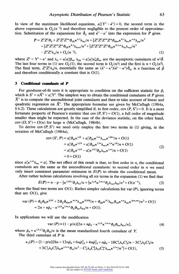
In view of the maximum likelihood equations, aK(Y' - iZ)= 0, the second term in the above expression is O,(n-A) and therefore negligible to the present order of approximation. Substitution of the expansions for Uij and .' - K' into the expression for P gives

P = Z'Zi+ii

+ Z'Zi' ikK k,llm/n + ZiZZmZ1aikK k'lmK n',p~l 2

+ ZZiZJZmZniykK kXkimnI /2 + ZZZ"ZAK k,',mX1nXmp/n 2

- ZZ'ZiZ/n + O,(n2-), (1)

where Zi= Y - K' and X= aa3s, k =

a•aa1~ 3s, are the asymptotic cumulants of n'i

. The last four terms in (1) are O, (1); the second term is O,(ni) and the first is n + O(n). The final term, Z'ZXhi4/n, essentially the same as (r- K')(Ki - K()KK ij, is a function of 3 and therefore conditionally a constant that is 0(1).

3 Conditional cumulants of P

For goodness-of-fit tests it is appropriate to condition on the sufficient statistic for 3, which is S' = nX' = aY'. The simplest way to obtain the conditional cumulants of P given X' is to compute the unconditional joint cumulants and then to take account of linear and quadratic regression on X'. The appropriate formulae are given by McCullagh (1984a, ? 6.2). These calculations are greatly simplified if, to first order, cov (P, S') = 0. It is a most fortunate property of Pearson's statistic that cov (P, S')= 0(1), a full order of magnitude smaller than might be expected. In the case of the deviance statistic, on the other hand, cov (D, S') = O(n) for large n (McCullagh, 1984b).

To derive cov (P, S') we need only employ the first two terms in (1) giving, in the notation of McCullagh (1984a),

cov (S', P) = a[OiK Ki'ik + afiklKmmnKiikn/n + O(1)

= ai?ikKiik +a'OklKl'm

AmnKinKk/l + 0(1)

(2)

SaroikKi'i'k - aKi,k,I jkA mKim/n + O(1) = 0+ 0(1)

since airK",Aim = aI. The net effect of this result is that, to first order in n, the conditional cumulants are the same as the unconditional cumulants: to second order in n we need only insert consistent parameter estimates in E(P) to obtain the conditional mean.

After rather tedious calculations involving all six terms in the expansion (1) we find that

E(P) = n -p - K iikiAkl K ,kK ',mniimnAkl 2+ O(n-1), (3) where the final two terms are 0(1). Rather simpler calculations for var (P), ignoring terms that are 0(1), give

var (P) = 1~Kii

' ,klK + 20jlklimK mnnpK iklp/n+OijkK k,lm'OrstK t'uuvK

ijmrsvl2 + 0(1)

= 2n + lnp4- Ki'+kK0'm'n if m kn/n + O(1).

In applications we will use the modification

var (P)- (1- p/n){2n + nlp4 - Ki,,kK KImn.if

•mkn/l}, (4)

where j14 = K i''k?'Jli?kdn

is the mean standardized fourth cumulant of Y. The third cumulant of P is

K3(P)= {1-p/n}[8n + 12np 4+6n 3+4n23 +P6 --18CAiiC/6n - 3C-A,C /n +

C3CAiiC3klK ,lrls

C2XijC3XklC3 XmmnK,''n 3] + O(1), (5)



64 P. McCULLAGH

where 2

""ic

-m, ijklmn2k ,mnai

13 K i~i~kK Ui[Tm mkn P23 = K' 3 K m&i[K&im&kn/n,

C = Ki'i'k Ajk,

C6 = K kmjk Im

6= K i,,kImn

kmn. The derivation of (5), which is based on only the first two terms of (1), is rather lengthy.

The first five terms give the third cumulant of Z'Z'iii: in addition to this, the products give 12 nonnegligible terms reducing to four by cancellation. The conditional cumulants of P are found by replacing all unknown quantities in (3), (4) and (5) by their maximum likelihood fitted values. The resulting conditional error terms are O(n-1), 0(1) and 0(1) respectively. The above results stem from McCullagh (1984a, ? 6.2) together with the sufficiency of the conditioning statistic.

4 Computation

For simplicity we consider only the case where the observations are independent with i

i Then cumulants Ki, K2, K313, K ....Then

3 1 •323/n, 04=

C

( n),/-,

P6 C K

/ Further, Ai/n is the approximate covariance matrix of {i~} the so-called linear predictor. In fact we need only the diagonal elements Ah,/n. Finally, let '/ =

K'i' xkijk[In = kC3hkIln,

which is the 'fitted value' after formal linear regression of the vector {( i /( i)2 n the model matrix A = {af} with weight vector {ZK}.

The first three conditional moments of P may be written

A=i A

Ani +i i

"43(is/n)

+ O(n-1), (6) E(P I S)- n--p - /.

K4

]_

- 3

var (PI S) = (1- p/n) 2n + n4

- C3 (1), (7)

K3(P S)=(1- p/n) 8n + 12n 4 +1On 2 ++n^6

A i A^A

A2ii A - 18 ,CYi -3 .i

- '3++3 i( 2

,i i i 3 +o(1). (8)

Note that y i9C' is the weighted regression sum of squares in the formal regression

described above, and P, is the estimate of P,. In the particular case where the observations are independent binomially distributed,

Y' - B(m1, -rri), expression (7) may be reduced to

var (P I -S)=(1-

p/n){2Z 1 + -1iv 1(I- )3W 1 + O(1), (9)

where = A(A VA)1A, =diag{}, is a projection matrix and CI -1(I -P)C3 is the residual weighted sum of squares in the supplementary regression of i /( )2 n A.

The first component in (9) is identically zero for ungrouped pure binary responses: the second component is identically zero if V-1C3 lies in the column space of A as occurs in one-way layouts. The second component in (9) will typically be small if the estimated regression parameters are nearly zero. In simulation studies with pure binary data (n = 50, p = 3) with two quantitative covariates and fairly strong regression effects, the second component in (9) varied between

2.0 and 7500, the average conditional variance




being about 400. Clearly, therefore, if Pearson's statistic is to be used in this way without

grouping it is essential to make use of the conditional variance appropriate to the

configuration of data observed. If the data are grouped prior to computing Pearson's statistic, the effect just described

persists though in a much weaker form. In simulation studies for binomial data with index mi = 10, n = 50, p = 3 and with weak regression effects ensuring all cell expectations were 3-5 or more, the conditional cumulants of P remained close to K1 = 47-30, K2 = 84-60 and K3/K3/2 = 0-37 compared with the nominal values of 47, 94 and 0-41 based on X2. The 2 47 - The

corresponding conditional cumulants with mi =6 were approximately 47-50, 78-34 and 0-33 with a little variation in the second and third conditional cumulants. In the latter case, all cell expectations were at least 2.1. With stronger regression effects, some cell expectations become small and the value of (9) becomes much more variable.

5 Example

For a simple application we use the data from the Ille-et-Vilaine study of oesophageal cancer given in Appendix 1 of Breslow & Day (1980). This is a retrospective case-control study with two risk factors, alcohol consumption and tobacco consumption each with four levels, and an additional variable, age, treated here as a qualitative variable with six levels. Of the 96 possible combinations of these factors only n = 88 were observed. The numbers observed in the remaining classes ranged from m = 1 to m = 60. Cell expectations ranged from very small to moderately large.

Pearson's statistic for the linear logistic model with main effects of the three variables is 86-46 on 76 degrees of freedom. The approximate conditional cumulants are Kl = 77-38, K2= 401-1 and p3 = 198 giving an approximate upper 5% point of 121-60 by Cornish- Fisher expansion. By the X26 approximation, the value 121-60 would correspond to a tail probability of about 0-001. In this example there is a strong potential for conflict between the two approximations. Fortunately, the observed value of 86-46 is near the centre of the distribution by either approximation and no conflict arises.

The reason for the very large value of K2 is not so much that some cell expectations are small but rather that the observed regression effects are very strong. For example the estimated effect on the log odds for cancer of heavy alcohol and heavy tobacco consumption are 3-6 and 1-6 respectively. In addition to these, the effect of a 50-year age difference is even stronger. The weighted residual sum of squares from the supplementary regression is 339-0 so that it is the second term and not the first that dominates in (9).

6 Two-way contingency tables

For a two-way contingency table with row totals si, i = 1, ..., r, and column totals ti, j = 1,... , c, Dawson (1954) has given the expression

2N(v - cr)(t - 7)/(N- 3) + N2or/(N- 1), (10)

where

v = (N- r)(r- 1)/(N- 1), . = (N- c)(c - 1)/(N- 1),

= N{X s ( 21 } (N -2), r = N{ t -2 /(N-2)



66 P. McCULLAGH

and N = i s = s ti, for the exact conditional variance of Pearson's goodness-of-fit statistic. In this case, the conditioning statistic is the set of row and column totals.

Strictly speaking, the asymptotic argument used in ? 3 is not applicable here because the number of parameters, r + c- 1, increases as the number of cells in the table increases. However it is interesting at least to note that the weighted residual sum of squares in the supplementary linear regression of NI(siti) on the two-way design is just

NoTr{(N- 2)2/N2} = Nor + O(N-1),

the essential ingredient of the second term in (10). Note that this term vanishes if either set of marginal totals is constant.

In the case of two-way contingency tables with either r = 2 or c = 2, the approximation (9) may be used, treating the data as binomially distributed with constant probability. This is typically a good deal more accurate than the corresponding approximation based on the Poisson log linear model. If both r > 2 and c > 2 the exact calculation seems preferable to the approximation (9).

7 Discussion

It is natural to raise the question of whether or not it is appropriate to use Pearson's statistic in the way we have described, without prior grouping. Most text books recom- mend grouping to some extent and this has the effect of greatly improving the X2

approximation. Selective grouping, on the other hand, could have obvious undesirable

consequences. The present calculations do not address the question of whether prior grouping is desirable. Instead, they show that if no grouping takes place and if the data are sparse then it is essential to use the conditional distribution rather than the marginal distribution for significance testing. Neither of these distributions will typically be close to

chi-square. The conditional moment calculations given here are appropriate when the residual

degrees of freedom is large and the number of fitted parameters is small. Under these conditions, the moment approximations appear to be very accurate. More refined approximations or even exact formulae are necessary for two-way and multi-way contingency tables where the number of fitted parameters may be large enough to introduce substan- tial errors in the calculations given here, particularly in (9). Finally, it would be very useful if similar calculations could be made for generalized linear models (McCullagh & Nelder, 1983). The result that Pearson's statistic is asymptotically independent of f has obvious implications for over-dispersion and it would be helpful to know whether this result continues to apply in the case of generalized linear models.

References

Breslow, N.E. & Day, N.E. (1980). Statistical Methods in Cancer Research, 1, The Analysis of Case-Control Studies. Lyon: IARC.

Dawson, R.B. (1954). A simplified expression for the variance of the x2-function on a contingency table. Biometrika 41, 280.

Haldane, J.B.S. (1937). The exact value of the moments of the distribution of X2 used as a test of goodness of fit when expectations are small. Biometrika 29, 133-143.

Haldane, J.B.S. (1939), The mean and variance of X2 when used as a test of homogeneity when expectations are small. Biometrika 31, 346-365.

Lewis, T., Saunders, I.W. & Westcott, M. (1984). Testing independence in a two-way contingency table: the moments of the chi-squared statistic and the minimum expected value. Biometrika 71, 515-522.

McCullagh, P. (1984a). Tensor notation and cumulants of polynomials. Biometrika 71, 461-476. McCullagh, P. (1984b). On the conditional distribution of goodness-of-fit statistics for discrete data. Unpub-

lished manuscript.




McCullagh, P. (1985). On the conditional cumulants of Pearson's statistic. GLIM Newsletter 10. To appear. McCullagh, P. & Nelder, J.A. (1983). Generalized Linear Models. London: Chapman and Hall.

Resum6

Les trois premiers moments conditionnels approximatifs de la statistique de Pearson sont derives pour des modules lin6aires arbitraires de familles exponentielles. L'approximation s'applique aux degr6s de libert6 nombreux et la variable conditionnante est la statistique exhaustive pour les parametres de regression. On d6montre que, quand les fr6quences theoretiques sont petites, la variance conditionelle peut varier le long de plusieurs ordres de magnitude selon la valeur de la statistique exhaustive. Un simple algorithme pour calculer les cumulants conditionnels qui implique un regression suppl6mentaire est d6taill6, et l'approximation d'Edgeworth est sugg6r6e pour l'estimation du niveau de significance.

[Received June 1984, revised September 1984]



Documents

On the Asymptotic Distribution of Pearson's Statistic in Linear Exponential-Family Models