ON THE BIRTH OF LIMIT CYCLES FOR NON{SMOOTH · PDF filewas given by Fatou in 1928 ... Let sign( u ) be the sign ... As usual r h denotes the gradient of the function h , @ x h denotes

http://www.gsd.uab.cat

ON THE BIRTH OF LIMIT CYCLES FOR

NON–SMOOTH DYNAMICAL SYSTEMS

JAUME LLIBRE1, DOUGLAS D. NOVAES2 AND MARCO A. TEIXEIRA2

Abstract. The main objective of this work is to develop, via Brower degree

theory and regularization theory, a variation of the classical averaging method

for detecting limit cycles of certain piecewise continuous dynamical systems. In

fact, overall results are presented to ensure the existence of limit cycles of such

systems. These results may represent new insights in averaging, in particular

its relation with non smooth dynamical systems theory. An application ispresented in careful detail.

1. Introduction and statement of the main results

The discontinuous differential systems, i.e. differential equations with discon-tinuous right–hand sides, is a subject that has been developed very fast these lastyears. It has become certainly one of the common frontiers between Mathematics,Physics and Engineering. Thus certain phenomena in control systems [2], impactand friction mechanics [6], nonlinear oscillations [1, 22], economics [13, 16], and bi-ology [3, 18], are the main sources of motivation of their study, see for more detailsTeixeira [27]. A recent review appears in [30].

The knowledge of the existence or not of periodic solutions is very important forunderstanding the dynamics of differential systems. One of good tools for studythe periodic solutions is the averaging theory, see for instance the books of Sandersand Verhulst [25] and Verhulst [29]. We point out that the method of averaging isa classical and matured tool that provides a useful means to study the behaviourof nonlinear smooth dynamical systems. The method of averaging has a long his-tory that starts with the classical works of Lagrange and Laplace who providedan intuitive justification of the process. The first formalization of this procedurewas given by Fatou in 1928 [10]. Very important practical and theoretical contri-butions in the averaging theory were made by Krylov and Bogoliubov [5] in the1930s and Bogoliubov [4] in 1945. The principle of averaging has been extendedin many directions for both finite- and infinite-dimensional differentiable systems.The classical results for studying the periodic orbits of differential systems needat least that those systems be of class C2. Recently Buica and Llibre [8] extendedthe averaging theory for studying periodic orbits to continuous differential systemsusing mainly the Brouwer degree theory.

Corresponding author Douglas D. Novaes: Departamento de Matematica, Universidade Estad-

ual de Campinas, Caixa Postal 6065, 13083–859, Campinas, SP, Brazil. Tel. +55 19 991939832,

Fax. +55 19 35216094, email: [email protected]

2010 Mathematics Subject Classification. 37G15, 37C80, 37C30.

Key words and phrases. periodic solution, averaging theory, discontinuous differential system.

1

This is a preprint of: “On the birth of limit cycles for non-smooth dynamical systems”, JaumeLlibre, Douglas D. Novaes, Marco Antonio Teixeira, Bull. Sci. Math., vol. 139, 229–244, 2015.DOI: [10.1016/j.bulsci.2014.08.011]

10.1016/j.bulsci.2014.08.011

2 J. LLIBRE, D.D. NOVAES AND M.A. TEIXEIRA

The main objective of this paper is to extend the averaging theory for studyingperiodic orbits to discontinuous differential systems using again the Brouwer degree.

Let D be an open subset of Rn. We shall denote the points of R ×D as (t, x),and we shall call the variable t as the time. Let h : R ×D → R be a C1 functionhaving the 0 ∈ R as a regular value, and let Σ = h−1(0). Given p ∈ Σ we denoteits connected component in Σ by Σp.

Let X,Y : R×D → Rn be two continuous vector fields. Assume that the func-tions h, X and Y are T–periodic in the variable t. Now we define a discontinuouspiecewise differential system

(1) x′(t) = Z(t, x) =

{X(t, x) if h(t, x) > 0,

Y (t, x) if h(t, x) < 0.

We concisely denote Z = (X,Y )h.

Here we deal with a different formulation for the discontinuous differential system(1). Let sign(u) be the sign function defined in R \ {0} as

sign(u) =

{1 if u > 0,

−1 if u < 0.

Then the discontinuous differential system (1) can be written using the functionsign(u) as

(2) x′(t) = Z(t, x) = F1(t, x) + sign(h(t, x))F2(t, x),

where

F1(t, x) =1

2(X(t, x) + Y (t, x)) and F2(t, x) =

1

2(X(t, x)− Y (t, x)) .

To work with the discontinuous differential system (2) we should introducethe regularization process, where the discontinuous vector field Z(t, x) is approx-imated by an one–parameter family of continuous vector fields Zδ(t, x) such thatlimδ→0 Zδ = Z(t, x).

In [26] Sotomayor and Teixeira introduced a regularization for the discontinuousvector fields in R2 having a line of discontinuity and, using this technique, theyproved generically that its regularization provides the same extension of the orbitsthrough the line of discontinuity that the one given by the Filippov’s rules, see [11].Later on Llibre and Teixeira [24] studied the regularization of generic discontinu-ous vector fields in R3 having a surface of discontinuity, and proved that limδ→0 Zδ

essentially agrees with Filippov’s convention in dimension three. Finally, in [27]Teixeira generalized the regularization procedure to finite dimensional discontinu-ous vector fields.

In [21] Llibre, da Silva and Teixeira studied singular perturbations problems indimension three which are approximations of discontinuous vector fields provingthat the regularization process developed in [24] produces a singular problem forwhich the discontinuous set is a center manifold, moreover, they proved that thedefinition of sliding vector field coincides with the reduced problem of the corre-sponding singular problem for a class of vector fields.

In general, a transition function is used in these regularizations to average thevector fields X and Y on the set of discontinuity in order to get a family of continuousvector fields that approximates the discontinuous one.

AVERAGING METHODS IN DISCONTINUOUS DIFFERENTIAL SYSTEMS 3

A continuous function φ : R → R is a transition function if φ(u) = −1 foru ≤ −1, φ(u) = 1 for x ≥ 1 and φ′(u) > 0 if u ∈ (−1, 1). The φ–regularization ofZ = (X,Y )h is the one–parameter family of continuous functions Zδ with δ ∈ (0, 1]given by

Zδ(t, x) =1

2(X(t, x) + Y (t, x)) +

1

2φδ(h(t, x)) (X(t, x)− Y (t, x)) ,

with

(3) φδ(u) = φ(uδ

).

Note that for all (t, x) ∈ (R×D)\Σ we have that limδ→0 Zδ(t, x) = Z(t, x).

The formulation (2) of the discontinuous differential system (1) admits a naturalregularization. Define the transition function φ as

(4) φ(u) =

1 if u ≥ 1,

u if − 1 < u < 1,

−1 if u ≤ −1.

Let φδ : R → R be the continuous function defined in (3). It is clear that

(5) limδ→0

φδ(u) = sign(u),

andZδ(t, z) = F1(t, x) + φδ(h(t, x))F2(t, x),

is the φ–regularization of the discontinuous differential system (1).

As usual ∇h denotes the gradient of the function h, ∂xh denotes the gradient ofthe function h restricted to the variable x and ∂th denotes the partial derivative ofthe function h with respect to the variable t.

Our main results are given in the next theorems. Its proof uses the theory ofBrouwer degree for finite dimensional spaces (see the appendix A for a definitionof the Brouwer degree dB(f, V, 0)), and is based on the averaging theory for non–smooth differential system stated by Buica and Llibre [8] (see Appendix B).

Theorem A. We consider the following discontinuous differential system

(6) x′(t) = εF (t, x) + ε2R(t, x, ε),

withF (t, x) = F1(t, x) + sign(h(t, x))F2(t, x),

R(t, x, ε) = R1(t, x, ε) + sign(h(t, x))R2(t, x, ε),

where F1, F2 : R×D → Rn, R1, R2 : R×D × (−ε0, ε0) → Rn and h : R×D → Rare continuous functions, T–periodic in the variable t and D is an open subset ofRn. We also suppose that h is a C1 function having 0 as a regular value.

Define the averaged function f : D → Rn as

(7) f(x) =

∫ T

0

F (t, x)dt.

We assume the following conditions.

(i) F1, F2, R1, R2 and h are locally Lipschitz with respect to x;(ii) there exists an open bounded set C ⊂ D such that, for |ε| > 0 sufficiently

small, every orbit starting in C reaches the set of discontinuity only at itscrossing regions (crossing hypothesis).


(iii) for a ∈ C with f(a) = 0, there exist a neighbourhood U ⊂ C of a such thatf(z) 6= 0 for all z ∈ U\{a} and dB(f, U, 0) 6= 0.

Then, for |ε| > 0 sufficiently small, there exists a T–periodic solution x(t, ε) ofsystem (6) such that x(0, ε) → a as ε → 0.

Theorem A is proved in section 2.

In order to stablish a theorem with weaker hypotheses we denote by D0 the setof points z ∈ D such that the map hz : t ∈ [0, T ] 7→ h(t, z) has only isolated zeros.Clearly Int(D0) 6= ∅.Theorem B. In addition to the assumptions of Theorem (A) unless condition (ii)we assume the following hypothesis.

(ii′) there exists an open bounded set C ⊂ D0 such that, for ε > 0 sufficientlysmall, every orbit starting in C reaches the set of discontinuity only at itscrossing regions.

Then, for ε > 0 sufficiently small, there exists a T–periodic solution x(t, ε) of system(6) such that x(0, ε) → a as ε → 0.

Theorem B is proved in section 2.

Remark 1. Assuming the hypotheses of Theorem A, we have that for ε = 0 itssolutions starting in C, i.e. straight lines {(t, z) : t ∈ R} for z ∈ C, reaches the setof discontinuity only at its crossing region. This fact is not necessarily true whenwe assume the hypotheses of Theorem B, because the crossing hypothesis holds onlyfor ε > 0. This is the main difference between Theorems A and B. Neverthelesswe shall see that to prove both theorems we just have to guarantee that the maphz : t ∈ [0, T ] 7→ h(t, z) for z ∈ C has only isolated zeros. After that the prooffollows similarly for both theorems.

Proposition 2. Assume that ∂th(t, x) 6= 0 for each (t, x) ∈ Σ. Then hypothesis(ii) holds.

Proposition 3. Assume that for each p ∈ Σ such that ∂th(p) = 0 there exists acontinuous positive function ξp : R×D → R for which the inequality

(∂th〈∂xh, F1〉+ ε

〈∂xh, F1〉2 − 〈∂xh, F2〉22

)(t, x) ≥ εξp(t, x)

holds for each (t, x) ∈ Σp. Then hypothesis (ii′) holds.

It is worthwile to say that the averaging theory appears as a very useful toolin discontinuous dynamical systems. For example, in [23], lower bounds for themaximum number of limit cycles for the m–piecewise discontinuous polynomial dif-ferential equations was provided using the averaging theory. In [9] the averagingtheory was used to study the bifurcation of limit cycles from discontinuous pertur-bations of two and four dimensional linear center in Rn. Also, in [20], the averagingtheory was applied to study the number of limit cycles of the discontinuous piece-wise linear differential systems in R2n with two zones separated by a hyperplane.

In Theorems A and B we have extended to general discontinuous differentialsystems the ideas used in the previous mentioned papers for particular discontinuousdifferential systems.

Now an application of Theorem A to a class of discontinuous piecewise lineardifferential systems is given. Such systems have been studied recently by Han and


Zhang [12], and Huan and Yuang [14], among other papers. In [12] some resultsabout the existence of two limit cycles appeared, so that the authors conjecturedthat the maximum number of limit cycles for this class of piecewise linear differ-ential systems is exactly two. This conjecture is analogous to Conjecture 1 in thediscussion of Tonnelier in [28]. However, by considering a specific family of dis-continuous PWL differential systems with two linear zones sharing the equilibriumposition, in [14] strong numerical evidence about the existence of three limit cycleswas obtained, and a proof was provided by Llibre and Ponce [19]. This examplerepresents up to now the first discontinuous piecewise linear differential systemwith two zones and 3 limit cycles surrounding a unique equilibrium. Now we shallprovide a new proof of the existence of these three limit cycles through TheoremA.

In polar coordinates (r, θ) given by x = r cos θ and y = r sin θ, the planar discon-tinuous piecewise linear differential system with two zones separated by a straightline corresponding to the system studied in the paper [19] is

(8)dr

dθ= F (θ, r) =

ε19

50r if r cos θ ≥ 1,

ε2300 cos(2θ)− 4623 sin(2θ)− 300

1500r if r cos θ < 1,

where we have multiplied the right hand side of the system of [19] by the smallparameter ε. Our main contribution in this application is to provide the explicitanalytic equations defining the limit cycles of the discontinuous piecewise lineardifferential system with two zones (8).

Theorem 4. Any limit cycle of the discontinuous piecewise linear differential sys-tem with two zones (8) which intersects the straight line x = 1 in two points (r0, θ0)and (r1, θ1) with −π/2 < θ0 < 0 < θ1 < π/2, rk cos θk = 1 for k = 0, 1, and r0 > 1and θ1 must satisfy the following two equations

(9)

exp

(19(θ1 − θ0)

50

)r0 cos θ1 − 1 = 0,

19(θ1 − θ0)

50+

1

5arctan

(1

15sec θ0(23 cos θ0 − 100 sin θ0)

)

−1

5arctan

(1

15sec θ1(23 cos θ1 − 100 sin θ1)

)

−1

2log(|4623 cos(2θ0) + 2300 sin(2θ0)− 5377|)

+1

2log(|4623 cos(2θ1) + 2300 sin(2θ1)− 5377|)− 2π

5= 0,

where θ0 = arccos(1/r0)− π, and the determination of the arctan is in the interval(−π/2, π/2) and of the arccos in the interval (0, π).

On the other hand, any limit cycle of system (8) which intersects the straightline x = 1 in two points (r0, θ0) and (r1, θ1) with 0 < θ0 < θ1 < π/2, rk cos θk = 1for k = 0, 1, and r0 > 1 and θ1 must satisfy the equations (9), but now in bothequations θ0 = arccos(1/r0).

We recall that a limit cycle of system (8) is an isolated periodic orbit of thatsystem in the set of all periodic orbits of the system. It is well known that the


-6 -4 -2

-1.5

-1.0

-0.5

0.5

1.0

1.5

x = 1

Figure 1. The three limit cycles surrounding the origin.

study of the limit cycles of the differential systems in dimension two is one of themain problems of the qualitative theory of differential systems in dimension two,see for instance the surveys of Ilyashenko [15] and Jibin Li [17].

In fact, as we shall see in the proof of Theorem 4 equations (9) have threesolutions, providing the three limit cycles of Figure 1.

2. Proofs of Propositions 2 and 3 and Theorems A and B

Proof of Proposition 2. System (6) can be written as the autonomous system

τ ′

x′

=

{X(τ, x) if h(τ, x) > 0,

Y (τ, x) if h(τ, x) < 0,

in R×D, where

X(τ, x) =

1

ε(F1(τ, x) + F2(τ, x)) + ε2(R1(τ, x, ε) +R2(τ, x, ε))

,

Y (τ, x) =

1

ε(F1(τ, x)− F2(τ, x)) + ε2(R1(τ, x, ε)−R2(τ, x, ε))

.


So

(10)

(Xh)(Y h) = 〈∇h,X〉〈∇h, Y 〉= (∂th)

2 + ε2∂th〈∇xh, F1〉+ε2

(2∂th〈∇xh,R1〉+ 〈∇xh, F1〉2 − 〈∇xh, F2〉2

)

+ε32 (〈∇xh, F1〉〈∇xh,R1〉 − 〈∇xh, F2〉〈∇xh,R2〉)+ε4

(〈∇xh,R1〉2 − 〈∇xh,R2〉2

).

Let x(t, z) be the solution of the system (6) such that x(0, z) = z. Fixed an openbounded subset U ⊂ D0 we define the compact subset K = {(t, x(t, z)) : (t, z) ∈[0, T ]× U} ⊂ [0, T ]×D.

Hence, we can choose |ε0| > 0 sufficiently small such that (Xh)(Y h)(t, x) > 0

for every (t, x) ∈ K ∩ Σ and ε ∈ (−ε0, ε0). Indeed (∂th(t, x))2is a continuous

positive function in R × D so there exists κ0 > 0 such that (∂th(t, x))2> κ0 for

every (t, x) ∈ K. �

Proof of Proposition 3. Consider the notation of the proof of Proposition 2. From(10) we also conclude that

(Xh)(Y h) =(∂th+ ε2〈∇xh,R1〉

)2

+2ε

(∂th〈∇xh, F1〉+ ε

〈∇xh, F1〉2 − 〈∇xh, F2〉22

)+ ε3O(1).

Now, we note that K∩Σ has a finite number of connected components, since Σ is aregular manifold in [0, T ]×D. So we can choose a finite subset {p1, p2, . . . , pm} ⊂ Σsuch that ∂th(pi) = 0 for i = 1, 2, . . . ,m, Σpi

∩Σpj= ∅ for i 6= j, and ∂th(t, x) 6= 0

for every (t, x) ∈ Σ\ (Σp1∪ Σp2

· · ·Σpm). Thus for i = 1, 2, . . . ,m

(Xh)(Y h)(t, x) ≥ εξpi(t, x) + ε3O(1),

for every (t, x) ∈ Σpi. We can choose then εi > 0 sufficiently small such that

(Xh)(Y h)(t, x) > 0 for every (t, x) ∈ K ∩ Σpiand ε ∈ (0, εi). Indeed ξpi

is acontinuous positive function in R×D so there exists κi > 0 such that ξpi

(t, x) > κi

for every (t, x) ∈ K. Moreover, by the proof of Proposition 2, we can choose|ε0| > 0 sufficiently small such that (Xh)(Y h)(t, x) > 0 for every (t, x) ∈ K ∩Σ\ (Σp1

∪ Σp2∪ · · · ∪ Σpm

) and ε ∈ (−ε0, ε0).Hence, choosing ε = min{ε0, ε1, . . . , εm} we conclude that (Xh)(Y h)(t, x) > 0

for every (t, x) ∈ K ∩ Σ and ε ∈ (0, ε) �

For proving Theorems A and B we need some preliminary lemmas. As usual µdenotes the Lebesgue Measure.

The hypotheses (ii) and (ii′) of Theorem A and B respectively make assumptionson the Brouwer degree of the averaged function f . So we need to show that thefunction f is continuous in order that the Brouwer degree will be well defined, formore details see Appendix A.

Lemma 5. The averaged function (7) is continuous in C.

Proof. First of all we note that either the hypothesis (ii) Theorem A or (ii′) ofTheorem B implies that the map hz : t 7→ h(t, z) has only isolated zeros for z ∈ C.Because the constant function t 7→ z is the solution of system (6) for ε = 0, thus,


from hypothesis (ii) of Theorem A, it reaches the set of discontinuity only at itscrossing region. From hypothesis (ii′) of Theorem B this conclusion is immediately.

For z ∈ C we define the sets A+z = {t ∈ [0, T ] : h(t, z) > 0}, A−

z = {t ∈ [0, T ] :h(t, z) < 0}, and A0

z = {t ∈ [0, T ] : h(t, z) = 0}. We note that µ(A0(z)

)= 0,

since the map hz : t 7→ h(t, z) has only isolated zeros for z ∈ C. Moreover [0, T ] =

A+(z) ∪A−(z).Now, fix z0 ∈ C, for z ∈ C in some neighborhood of z0, we estimate

|f(z)− f(z0)| ≤∫ T

0

|F1(t, z0)− F1(t, z)|dt

+

∫ t

0

|sign(h(t, z0))F2(t, z0)− sign(h(t, z))F2(t, z)|dt

≤ TL|z0 − z|+

∫

A+z0

∩A+z

|F2(t, z0)− F2(t, z)|dt+∫

A−z0

∩A−z

|F2(t, z0)− F2(t, z)|dt

+

∫

A+z0

∩A−z

|F2(t, z0) + F2(t, z)|dt+∫

A−z0

∩A+z

|F2(t, z0) + F2(t, z)|dt

≤ 3T |z0 − z|+(µ(A+

z0 ∩A−z

)+ µ

(A−

z0 ∩A+z

))M,

where L is the Lipschitz constant of F1 and M = max{F2(t, z) : (t, z) ∈ [0, T ] ×U} < ∞. It is easy to see that µ

(A+

z0 ∩A−z

)→ 0 and µ

(A−

z0 ∩A+z

)→ 0 when

z → z0. So the lemma is proved. �

Let a be the point in hypothesis (iii) of Theorems A and B. By Lemma 5 thereexists a neighborhood U ⊂ C of a such that f is continuous in U . Hence, byTheorems 10 and 11 (see Appendix A), there exists a unique map that satisfiesthe properties of the Brouwer degree for the function f(z) with z ∈ U , because0 /∈ f(∂U). This map is denoted by dB(f, U, 0).

Lemma 6. For |ε| > 0 (or ε > 0) sufficiently small the solutions of system (6) (inthe sense of Filippov) starting in C are uniquely defined.

To prove Lemma 6 we will need the following proposition, that has been provedin Corollary 1 of section 10 of chapter 1 of [11]. Define

S+ = {(t, x) ∈ R×D : h(t, x) > 0},S− = {(t, x) ∈ R×D : h(t, x) < 0}.

Note that R×D = S− ∪ Σ ∪ S+.

Proposition 7. For every point of the manifold Σ where (Xh)(Y h) > 0, there isa unique solution passing either from S− into S+, or from S+ into S−.

Proof of Lemma 6. The proof follows immediately from Proposition 7 and hypoth-esis (ii). �

Instead of working with the discontinuous differential system (6) we shall workwith the continuous differential system

(11) x′(t) = εFδ(t, x) + ε2Rδ(t, x, ε),


whereFδ(t, x) = F1(t, x) + φδ(h(t, x))F2(t, x),

Rδ(t, x, ε) = R1(t, x, ε) + φδ(h(t, x))R2(t, x, ε),

and φδ : R → R is the continuous function defined in (3) and (4), and satisfying(5).

For system (11) the averaged function is defined as

fδ(z) =

∫ T

0

Fδ(t, x)dt.

We need to guarantee that hypothesis (i) of Theorem 12 (see appendix A) holdsfor the functions Fδ and Rδ. For this purpose we prove the following lemma.

Lemma 8. For δ ∈ (0, 1] the function φδ : R → R defined in (3) with φ given by(4) is globally 1/δ–Lipschitz; i.e. for all u1, u2 ∈ R we have that |φδ(u1)−φδ(u2)| ≤(1/δ)|u1 − u2|.Proof. If u1 ≤ −δ < δ ≤ u2, then |φδ(u1)−φδ(u2)| = 2 = (1/δ)2δ ≤ (1/δ)|u1−u2|.

If u1, u2 ≤ −δ or u1, u2 ≥ δ, then |φδ(u1)− φδ(u2)| = 0 ≤ (1/δ)|u1 − u2|.Assume that u1 ∈ (−δ, δ). If |u2| < δ, then |φδ(u1) − φδ(u2)| = (1/δ)|u1 − u2|;

and if |u2| ≥ δ, then |φδ(u1)−φδ(u2)| ≤ max{|1/δ|, |1/u2|}|u1−u2| ≤ (1/δ)|u1−u2|.This completes the proof of the lemma. �Proposition 9. For δ ∈ (0, 1] the functions Fδ and Rδ are locally Lipschitz withrespect to the variable x.

Proof. Let K ⊂ D be a compact subset. Denote M = sup{|F2(t, x)| : (t, x) ∈[0, T ] × K}, which is well defined by continuity of the function (t, x) 7→ |F2(t, x)|and compactness of the set [0, T ] × K. For x1 and x2 in K where F1 and h arelocally Lipschitz and by Lemma 8, we have

|Fδ(t, x1)− Fδ(t, x2)| = |F1(t, x1)− F1(t, x2)

+φδ(h(t, x1))F2(t, x1)− φδ(h(t, x2))F2(t, x2)|≤ |F1(t, x1)− F1(t, x2)|

+|φδ(h(t, x1))F2(t, x1)− φδ(h(t, x2))F2(t, x2)|≤ L|x1 − x1|+ |φδ(h(t, x1))||F2(t, x1)− F2(t, x2)|

+|F2(t, x2)||φδ(h(t, x1))− φδ(h(t, x2))|≤ 2L|x1 − x2|+

M

δ|h(t, x1)− h(t, x2)|

≤(2L+

ML

δ

)|x1 − x2| = Lδ|x1 − x2|.

Here L is the maximum between the Lipschitz constant of the functions F1 and F2.The proof for Rδ is analogous. �Now we are ready to prove Theorems A and B. We shall prove only theorem A.

The proof of Theorem B is completely analogous.

Proof of Theorem A. We will study the Poincare maps for the discontinuous dif-ferential system (6) and for the continuous differential system (11). For eachz ∈ C, let x(t, z, ε) denote the solution (in the sense of Filippov) of system (6)


t

Σ

Rn

nT≡0

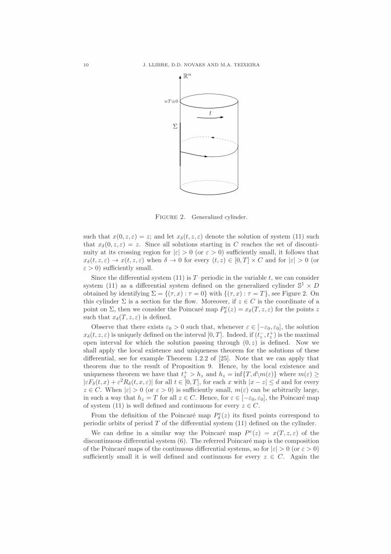
Figure 2. Generalized cylinder.

such that x(0, z, ε) = z; and let xδ(t, z, ε) denote the solution of system (11) suchthat xδ(0, z, ε) = z. Since all solutions starting in C reaches the set of disconti-nuity at its crossing region for |ε| > 0 (or ε > 0) sufficiently small, it follows thatxδ(t, z, ε) → x(t, z, ε) when δ → 0 for every (t, z) ∈ [0, T ] × C and for |ε| > 0 (orε > 0) sufficiently small.

Since the differential system (11) is T–periodic in the variable t, we can considersystem (11) as a differential system defined on the generalized cylinder S1 × Dobtained by identifying Σ = {(τ, x) : τ = 0} with {(τ, x) : τ = T}, see Figure 2. Onthis cylinder Σ is a section for the flow. Moreover, if z ∈ C is the coordinate of apoint on Σ, then we consider the Poincare map P ε

δ (z) = xδ(T, z, ε) for the points zsuch that xδ(T, z, ε) is defined.

Observe that there exists ε0 > 0 such that, whenever ε ∈ [−ε0, ε0], the solutionxδ(t, z, ε) is uniquely defined on the interval [0, T ]. Indeed, if (t−z , t

+z ) is the maximal

open interval for which the solution passing through (0, z) is defined. Now weshall apply the local existence and uniqueness theorem for the solutions of thesedifferential, see for example Theorem 1.2.2 of [25]. Note that we can apply thattheorem due to the result of Proposition 9. Hence, by the local existence anduniqueness theorem we have that t+z > hz and hz = inf{T, d\m(ε)} where m(ε) ≥|εFδ(t, x) + ε2Rδ(t, x, ε)| for all t ∈ [0, T ], for each x with |x− z| ≤ d and for everyz ∈ C. When |ε| > 0 (or ε > 0) is sufficiently small, m(ε) can be arbitrarily large,in such a way that hz = T for all z ∈ C. Hence, for ε ∈ [−ε0, ε0], the Poincare mapof system (11) is well defined and continuous for every z ∈ C.

From the definition of the Poincare map P εδ (z) its fixed points correspond to

periodic orbits of period T of the differential system (11) defined on the cylinder.

We can define in a similar way the Poincare map P ε(z) = x(T, z, ε) of thediscontinuous differential system (6). The referred Poincare map is the compositionof the Poincare maps of the continuous differential systems, so for |ε| > 0 (or ε > 0)sufficiently small it is well defined and continuous for every z ∈ C. Again the


fixed points of P ε(z) correspond to periodic orbits of the discontinuous differentialsystem (6).

Clearly (from above considerations), for z ∈ C and for |ε| > 0 (or ε > 0)sufficiently small, the pointwise limit of the Poincare map P ε

δ (z) of system (11),when δ → 0 is the Poincare map P ε(z) of system (6).

By definition the continuous differential system (11) is C2 in the variable ε. Sowe do the Taylor expansion of the Poincare map of system (11) around ε up toorder two, and we get

(12) P εδ (z) = z + εfδ(z) +O(ε2),

where fδ(z) is the averaged function of the continuous differential system (11), formore details see for instance [8]. Due to (5) we obtain that the pointwise limit inΣ of the function fδ, when δ → 0 is the function f .

Let a ∈ U be the point satisfying hypotheses (ii) of Theorem A. Thereforef(z) 6= 0 for all z ∈ V \{a}. Define f0 = f |V , we know that f0 is continuous byLemma 5. Then, we consider the continuous homotopy {fδ|V , 0 ≤ δ ≤ 1}. Weclaim that there exists a δ0 ∈ (0, 1] such that 0 /∈ fδ(∂V ) for all δ ∈ [0, δ0]. Now weshall prove the claim.

As usual N denotes the set of positive integers. Suppose that there exists asequence (zm)m∈N in ∂U such that f 1

m(zm) = 0. As the sequence (zm) is contained

in the compact set ∂U , so there exists a subsequence (zmℓ)ℓ∈N such zmℓ

→ z0 ∈ ∂U .Consequently we obtain that f(z0) = 0, in contradiction with the hypotheses (ii)of Theorem A. Hence, the claim is proved.

From the above claim and the property (iii) of Theorem 10 (see Appendix A)we conclude that dB(fδ, V, 0) 6= 0 for 0 ≤ δ ≤ δ0. Therefore, by the property (i) ofTheorem 10 we obtain that 0 ∈ fδ(V ), so there exists aδ ∈ U such that fδ(aδ) = 0.Since, by continuity, there exists the limδ→0 aδ and it is a zero of the functionf0 = f |U . This limit is the point a of the hypotheses (ii) of Theorem A, because ais the unique zero of f0 in U .

In summary, in order that for every δ ∈ (0, δ0] the averaged function fδ satisfythe assumptions (ii) of Theorem 12 (see Appendix B). So it only remains to showthat in U we have that fδ(z) 6= 0 for all z ∈ V \ {aδ}. But this can be achieved ina complete similar way as we proved the above claim. Hence, by Proposition 9 forevery δ ∈ (0, δ0] the continuous differential system (11) satisfies all the assumptionsof Theorem 12. Hence, for |ε| sufficiently small there exists a periodic solutionxδ(t, ε) of the continuous differential system (11) such that z(δ,ε) := xδ(0, ε) → aδwhen ε → 0.

Now, from (12) the point z(δ,ε) is a fixed point of the Poincare map P εδ (z), i.e.

P εδ (z(δ,ε)) = z(δ,ε). Since limδ→0 P

εδ (z) = P ε(z), it follows that zε = limδ→0 z(δ,ε) is

a fixed point of the Poincare map P ε(z). So, the discontinuous differential system(6) has a periodic solution x(t, ε) such that zε = x(0, ε) → a as ε → 0. Thereforethe theorem is proved. �

3. Application

In this section we shall prove Theorem 4, by applying Theorem A to the discon-tinuous differential system (8). So, we must compute the integral (7), which for


system (8) becomes

(13) f(r) =

∫ 2π

0

F (θ, r) dθ,

where the function F (θ, r) is given in (8).

The solution of the differential system (8) in the half–plane x = r cos θ ≥ 1starting at the point (r0, θ0) with r0 cos θ0 = 1 and θ0 ∈ (−π/2, 0) is

r(θ) = exp

(19(θ − θ0)

50

)r0.

Therefore, at the point (r1, θ1) with r1 cos θ1 = 1 and θ1 ∈ (0, π/2) we have that

exp

(19(θ1 − θ0)

50

)r0 cos θ1 = 1.

This equation coincides with the first equation of (9).

Now computing the integral (13) we obtain exactly the right hand side of thesecond equation of (9) multiplied by r. According to Theorem A we must find thezeros of this last expression. Since r cannot be zero the equation for the zeros isreduced exactly to the second equation of (9). In short, by Theorem A we haveproved that a periodic orbit of system (8) intersects the straight line x = 1 in twopoints (r0, θ0) and (r1, θ1) with θ0 ∈ (−π/2, 0), θ1 ∈ (0, π/2), rk cos θk = 1 fork = 0, 1, and r0 > 1 and θ1 must satisfy the equations (9).

In [19] it is proved that the discontinuous differential equation (8) has three limitcycles (i) and that the their points (r0, θ0) and (r1, θ1) are approximately for theinner limit cycle of Figure 1

(14) r0 = 1.013330663139.., θ0 = 0.162383740477.., θ1 = 0.5541676264624..;

for the middle limit cycle of Figure 1

(15) r0 = 1.003945075086.., θ0 = −0.088680876377.., θ1 = 0.768002346543..;

for the external limit cycle of Figure 1

(16) r0 = 1.111870463116.., θ0 = −0.452434880837.., θ1 = 1.034197922817...

It is easy to check that (14), (15) and (16) satisfies the two equations (9). Hence,Theorem 4 is proved.

Appendix A: Basic results on the Brouwer degree

In this appendix we present the existence and uniqueness result from the degreetheory in finite dimensional spaces. We follow the Browder’s paper [7], where areformalized the properties of the classical Brouwer degree.

Theorem 10. Let X = Rn = Y for a given positive integer n. For bounded opensubsets V of X, consider continuous mappings f : V → Y , and points y0 in Ysuch that y0 does not lie in f(∂V ) (as usual ∂V denotes the boundary of V ). Thento each such triple (f, V, y0), there corresponds an integer d(f, V, y0) having thefollowing three properties.

(i) If d(f, V, y0) 6= 0, then y0 ∈ f(V ). If f0 is the identity map of X onto Y ,then for every bounded open set V and y0 ∈ V , we have

d(f0∣∣V, V, y0

)= ±1.


(ii) (Additivity) If f : V → Y is a continuous map with V a bounded open setin X, and V1 and V2 are a pair of disjoint open subsets of V such that

y0 /∈ f(V \(V1 ∪ V2)),

then,

d (f0, V, y0) = d (f0, V1, y0) + d (f0, V1, y0) .

(iii) (Invariance under homotopy) Let V be a bounded open set in X, and con-sider a continuous homotopy {ft : 0 ≤ t ≤ 1} of maps of V in to Y . Let{yt : 0 ≤ t ≤ 1} be a continuous curve in Y such that yt /∈ ft(∂V ) for anyt ∈ [0, 1]. Then d(ft, V, yt) is constant in t on [0, 1].

Theorem 11. The degree function d(f, V, y0) is uniquely determined by the threeconditions of Theorem 10.

For the proofs of Theorems 10 and 11 see [7].

Appendix B: Basic results on averaging theory

In this appendix we present the basic result from the averaging theory that weshall need for proving the main results of this paper. For a general introduction toaveraging theory see for instance the book of Sanders and Verhulst [25].

Theorem 12. We consider the following differential system

(17) x′(t) = ε F (t, x) + ε2 R(t, x, ε),

where F : R×D → Rn and R : R× U × (−εf , εf ) → Rn are continuous functions,T -periodic in the first variable and D is an open subset of Rn. We define theaveraged function f : D → Rn as

(18) f(x) =

∫ T

0

F (s, x)ds,

and assume that

(i) F and R are locally Lipschitz with respect to x;(ii) for a ∈ D with f(a) = 0, there exist a neighborhood V of a such that

f(z) 6= 0 for all z ∈ V \{a} and dB(f, V, 0) 6= 0.

Then, for |ε| > 0 sufficiently small, there exist a T–periodic solution x(t, ε) of thesystem (17) such that x(0, ε) → a as ε → 0.

Theorem 12 for studying the periodic orbits of continuous differential systemshas weaker hypotheses than the classical result for studying the periodic orbits ofsmooth differential systems, see for instance Theorem 11.5 of Verhulst [29], whereinstead of (i) is assumed that

(j) F, R, DxF, D2xF and DxR are defined, continuous and bounded by a con-

stant M (independent of ε) in [0,∞)×D, −εf < ε < εf ;

and instead of (ii) it is required that

(jj) for a ∈ D with f(a) = 0 we have that Jf (a) 6= 0, where Jf (a) is theJacobian matrix of the function f at the point a.

For a proof of Theorem 12 see [8] section 3.


Acknowledgements

The first author is partially supported by a MICINN/FEDER grant MTM2008–03437, by a AGAUR grant number 2009SGR–0410, by ICREA Academia and FP7PEOPLE-2012-IRSES-316338 and 318999. The second author is partially sup-ported by a FAPESP–BRAZIL grant 2012/10231–7. The third author is partiallysupported by a FAPESP–BRAZIL grant 2007/06896–5. The first and third authorsare also supported by the joint project CAPES-MECD grant PHB-2009-0025-PC.

References

[1] A. A. Andronov, A.A. Vitt and S. E. Khaikin, Theory of oscillators, International Series

of Monographs In Physics 4, Pergamon Press, 1966.

[2] E. A. Barbashin, Introduction to the Theory of Stability (T. Lukes, Ed.), Noordhoff, Gronin-

gen, 1970.

[3] A. D. Bazykin, Nonlinear Dynamics of Interacting Populations, River-Edge, NJ: WorldScientific, 1998.

[4] N. N. Bogoliubov, On some statistical methods in mathematical physics, Izv. vo Akad.

Nauk Ukr. SSR, Kiev, 1945.

[5] N. N. Bogoliubov and N. Krylov, The application of methods of nonlinear mechanics in

the theory of stationary oscillations, Publ. 8 of the Ukrainian Acad. Sci. Kiev, 1934.

[6] B. Brogliato, Nonsmooth Mechanics, New York: Springer-Verlag, 1999.

[7] F. Browder, Fixed point theory and nonlinear problems, Bull. Amer. Math. Soc. 9 (1983),

1–39.

[8] A. Buica and J. Llibre, Averaging methods for finding periodic orbits via Brouwer degree,

Bulletin des Sciences Mathematiques 128 (2004), 7–22.

[9] P.T. Cardin, T. Carvalho and J. Llibre, Limit Cycles of discontinuous piecewise linear

differential systems, Int. J. Bifurcation and Chaos 21 (2011), 3181–3194.

[10] P. Fatou, Sur le mouvement d’un systame soumis a des forces a courte periode, Bull. Soc.

Math. France 56 (1928), 98–139.

[11] A. F. Filippov, Differential Equations with Discontinuous Righthand Side, Mathematics and

Its Applications, Kluwer Academic Publishers, Dordrecht, 1988.

[12] M. Han and W. Zhang, On Hopf bifurcation in non–smooth planar systems, J. of Differential

Equations 248 (2010), 2399–2416.

[13] C. Henry, Differential equations with discontinuous righthand side for planning procedure,

J. Econom. Theory 4 (1972), 541–551.

[14] S.M. Huan and X.S. Yang, The number of limit cycles in general planar piecewise linear

systems, Discrete Contin. Dyn. Syst. 32 (2012), 2147–2164.

[15] Y. Ilyashenko, Centennial history of Hilbert’s 16th problem, Bull. Amer. Math. Soc. 39

(2002), 301–354.

[16] T. Ito A Filippov solution of a system of differential equations with discontinuous right-handsides, Economic Letters 4 (1979), 349–354.

[17] J. Li, Hilbert’s 16th problem and bifurcations of planar polynomial vector fields, Internat. J.

Bifur. Chaos Appl. Sci. Engrg. 13 (2003), 47–106.

[18] V. Krivan, On the Gause predator–prey model with a refuge: A fresh look at the history,

Journal of Theoretical Biology 274 (2011), 67–73.

[19] J. Llibre and E. Ponce, Three limit cycles in discontinuous piecewise linear differential

systems with two zones, Dyn. Contin. Discrete Impuls. Syst. Ser. B Appl. Algorithms 19

(2012), 325–335.

[20] J. Llibre and F. Rong, On the number of limit cycles for discontinuous piecewise linear

differential systems in R2n with two zones, Int. J. of Bifurcation and Chaos 23 (2013),

1350024 7 pp.

[21] J. Llibre, P.R. da Silva and M.A. Teixeira, Regularization of discontinuous vector fields

on R3 via singular perturbation, J. Dynamics and Differential Equations 19 (2007), 309–331.

[22] N. Minorski, Nonlinear Oscillations, Van Nostrand, New York, 1962.

[23] J. Llibre and M.A. Teixeira, Limit cycles for m–piecewise discontinuous polynomial

Lienard differential equations, arXiv: [math.DS], preprint.


[24] J. Llibre and M.A. Teixeira, Regularization of discontinuous vector fields in dimension

three, Discrete and Continuous Dynamical Systems 3 (1997), 235–241.

[25] J. Sanders and F. Verhulst, Averaging method in nonlinear dynamical systems, Applied

Mathematical Sciences 59, Springer, 1985.

[26] J. Sotomayor and M.A. Teixeira, Regularization of Discontinuous Vector Field, Interna-

tional Conference on Differential Equation, Lisboa, 1995, World Sci. Publ., River Edge, NJ,

1998, pp 207–223.

[27] M.A. Teixeira, Perturbation theory for non–smooth systems, Encyclopedia of Complexity

and Systems Science 22, Springer, New York, 2009, pp 6697–6719.

[28] A. Tonnelier, The McKean’s caricature of the FitzHugh-Nagumo model I. The space-

clamped system, SIAM J. Appl. Math. 63 (2003), pp. 459–484.

[29] F. Verhulst, Nonlinear Differential Equations and Dynamical Systems, Universitext,

Springer, 1991.

[30] Various, Special issue on dynamics and bifurcations of nonsmooth systems Physica D 241

(2012), 1825–2082.

1 Departament de Matematiques, Universitat Autonoma de Barcelona, 08193 Bel-

laterra, Barcelona, Catalonia, Spain

E-mail address: [email protected]

2 Departamento de Matematica, Universidade Estadual de Campinas, Caixa Postal

6065, 13083–859, Campinas, SP, Brazil

E-mail address: [email protected], [email protected]

Documents

ON THE BIRTH OF LIMIT CYCLES FOR NON{SMOOTH · PDF filewas given by Fatou in 1928 ... Let sign( u ) be the sign ... As usual r h denotes the gradient of the function h , @ x h denotes