y. Chem. Thermodynamics 1971, 3, 19-34

On the calculation of the corrected temperature rise in isoperibol calorimetry. Modifications of the Dickinson extrapolation method and treatment of thermistor-thermometer resistance valuest

STUART R. GUNN

Lawrence Radiation Laboratory, University of California, Livermore, California 94550, U.S.A.

(Received 18 May 1970)

Rigorous parallel derivations and numerical examples are given for the Dickinson extra- polation method, for a previously described variation, and for a new, more convenient variation. The effect of a changed steady power input (heat of rotation, secondary reaction, or stirring change) is considered. Procedures for the direct use of thermistor resistance values are discussed, and numerical examples are given.

1. Introduction

In isoperibol calorimetry, the temperature change of the calorimeter during the main period of an experiment is generally not determined solely by the amount of heat liberated or absorbed by the process under investigation. A certain part of the change is due to heat exchange with the environment and to extraneous thermal effects within the calorimeter, such as heat of stirring, joule heating by an electrical thermo- meter, etc. The term "corrected temperature rise" is defined as the temperature change which the calorimeter would have experienced in the absence of these perturbations (neglecting thermal gradients within the calorimeter, the effect of which is minimized by the method of comparative measurements). This term, multi- plied by the energy equivalent of the calorimeter, gives the amount of heat attri- butable to the process under investigation.

Dickinson o 2) described a method of calculating the corrected temperature rise wherein tangents to the time-temperature curves at the beginning and end of the main period are extrapolated to a defined time such that the difference of their values at that time is equal to the corrected temperature rise. This "extrapolation time" is determined from graphical integration of the time-temperature curve during the main period. Such a method has significant advantages in many fields of calorimetry. Foremost amongst these is the rapidity of the calculation. Another advantage is

t Work performed under the auspices of the U.S. Atomic Energy Commission.

20 S.~R. GUNN

adaptability of the method to modern instrumental technique; it is frequently con- venient, with the usual electrical thermometer systems, to employ an amplifier and strip-chart recorder to display the whole time-temperature curve of the main period directly, rather than reconstruct the curve from intermittent readings. With reaction calorimeters of small size used for the measurement of rapid reactions, the temperature rise during the main period may be so rapid that adequate definition of the curve may not be attainable from the intermittent readings obtained, for example, by conventional use of a bridge and galvanometer. But the higher thermal leakage modulus which accompanies smaller dimensions requires a higher accuracy in integration of the main period, or determination of the extrapolation time, for a given overall accuracy.

This paper gives parallel derivations of the original Dickinson method, a variation described by Challoner, Gundry, and Meetham, (a) and a new variation which in many cases is more convenient. Numerical examples are given. Finally, the feasibility of using thermistor resistance values without conversion to temperatures is discussed and illustrated.

Regardless of the method used to calculate a corrected temperature rise, the validity of this rise as a means of comparing two experiments depends upon certain characteristics of the design of the calorimeter and of the experiment. These include particularly the requirements that temperature gradients within the calorimeter during the initial and final periods be sufficiently similar during the two experiments, and that the thermometer measures a temperature which gives a valid measure of heat exchange with the environment during the main period, at least on a relative basis for the two experiments. These problems have been considered by several authors(k-7) and will not be dealt with further here.

2. Derivations

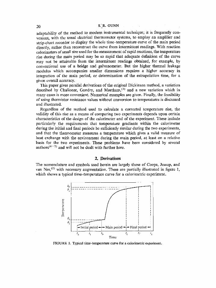
The nomenclature and symbols used herein are largely those of Coops, Jessup, and van Nes, (2) with necessary augmentation. These are partially illustrated in figure 1, which shows a typical time-temperature curve for a calorimetric experiment.

O f . . . . . . . . . . . . . . . . . . . . . . . . . . . . .

0c

¢ o

o~' 1 1 ¢ ' ~ I I

I f I r

0b . , . . . . . . . . . . . . . p i

i i i I

mitim period -,.-~-.,- Main perioa-~.--- final perioa -- i i J ,

t a t i t b t e tf t z Time

FIGURE 1. Typical time-temperature curve for a calorimetric experiment.

CORRECTED TEMPERATURE RISE IN ISOPERIBOL CALORIMETRY 21

The temperatures of the calorimeter during the initial, main, and final periods are designated 01, 02, and 0 a, respectively. Subscripts 1 and 3 are also used to denote extrapolations into the main period of equations decribing 0 for the initial and final periods. The rate of change of temperature during the initial and final periods is assumed to be described by Newton's law,

g = dO/dt = u + k(Oj - 0), (1) where

u = (2) Here p is the sum of all constant thermal powers in the calorimeter, due to stirring, evaporation, joule heating by the resistance thermometer, etc., e is the energy equivalent of the calorimeter and its contents, k is the thermal leakage modulus, and 0j is the effective jacket temperature. A convergence temperature 0~, which 0 approaches with increasing time, may be obtained by setting dO/dt = 0 in equation (1) and solving for 0:

ooo = oj + u / k . (3) Substitution of equation (3) into (1) gives

g = dO/dt = k(Ooo- 0). (4)

Integration of equation (4) for 01 and Oa gives

01 = 0~o - (000 - 05) exp { - k ( t - tb)}, (5)

03 = 0~o -- (0~o -- 0e) exp { -- k ( t - te)~ (6)

where 05 and 0o are the temperatures at the times t b and t~, which represent the begin- ning and end of the main period.

In the ensuing treatment, it will initially be assumed that u, k, and 0j are constant. In practice this assumption is almost always made and, although it is never strictly true, the net effect of deviations from it can be made very small if similar conditions are used for the calibration and the experimental measurements. Later, the effect of a change in u during the main period will be considered.

That component of the temperature change during the main period which is due to heat exchange with the environment and to the constant thermal powers p within the calorimeter is also described by equation (4). Hence the corrected temperature rise A0¢orr is given by

A O .... = 0 e - - 0 b - - ~ 0 ,

where t¢

50 = k S (0~o- 02) dt. tb

The thermal leakage modulus can be obtained from

k = ( g l - g O / ( O f - 0~), (9)

which is derived from (4); gi and gf are the values of dO/dt at the mean temperatures 0i and Of of the initial and final periods. The convergence temperature can also be obtained by rearranging (4):

0oo = Of d- g f /k --- Oi + gl/k. (10)

(7)

(8)

22 S.R. GUNN

In principle, single observed values of 0b and 0 e could be used in equation (7). In practice, it is much more preferable to use all of the time-temperature observations of the initial and final periods, fitted to (5) and (6), to obtain more reliable values of 0b and 0~. Equations (9) and (10) may be used first to calculate k and 0oo, after a preliminary fitting of the initial and final periods to obtain &, g~, 0~, and 0f.

Equations (5), (6), and (7) are exact insofar as the basic assumptions--that u, k, and 0. are constant--are valid. Because the exponents k ( t - - t b ) and k ( t - t ~ ) are generally quite small, (5) and (6) may be very closely approximated by quadratic equations which are easier to handle. (2) It is a still easier and common practice, however, to fit the points of the initial and final periods to straight lines,

Ot = 0[, + fi( t-- tb),

03 = O" + 9~(t- t~), either graphically or by least squares analysis. The (linear)" AO'¢orr is then defined as

t t AOcorr = 0 e - - O k - 8 0 ' ,

where te

80' = k' I ( 0 " - 0 2 ) dt, tb

k' = (o~- o3 / (0 f - 0i), 0 ' "k . . . . k' 0 ~ = f - l - g f / = O i - I - g i / .

"corrected

(5')

(6') temperature rise

(7')

(8')

(93 (10')

The difference of the two values of the corrected temperature rise, neglecting the usually small difference between 60 and 60', is

A0corr- A0tcorr = (0e -- Ore) -- (0b -- 0;). (11) For much work, the difference (A0'corr- A0corr ) is sufficiently small and sufficiently con- stant so that A0'~orr may be used in place of A0 .... . In particular, if the method of comparative measurements is being rigorously applied, the values of (0~-0 i ) and (0~ - 00 and the duration of the initial and final periods will be nearly the same for the two experiments being compared (combustion of benzoic acid and combustion of another substance, for example, or an electrical heating and a chemical reaction); hence the curvature of the initial and final periods, and consequently (0 b - 0~,), (0~- 0'~), and (A0 .... -A0'oorr), will be very closely similar.

We shall refer to the foregoing procedure as the "integration method." It is also known in various versions as the Regnault-Pfaundler method. Variations in opera- tional details involve mainly the fitting of the initial and final periods and the integration of the main period. We shall now consider the Dickinson method and its variations, designating these as "extrapolation methods."

EXTRAPOLATION METHOD A

Dickinson showed that

where A 0 . . . . = 0 3 x a - 01xa,

01xa = 0b "[- gb(txa-- tb),

03x a = 0# + g¢(txa-- te) ,

(12)

(13)

(14)

CORRECTED TEMPERATURE RISE IN ISOPERIBOL CALORIMETRY 23

if the time txa is selected so that txa te I (02--0b) dt = I (0~-02) dt, (15) tb txa

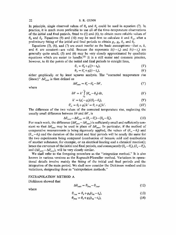
that is, so that areas A and B in figure 2(a) are equal. The proof is as follows.

A 2 0e B:2 /~I A, ° t

,, tb txa te

(a) Extrapolation method A

A. 2

t~, txb te

(b) Extrapolation method B

Of . . . . .

BT! 0i ~ -'r '~ i

t i t b txa t e tf S

(c) Extrapolation method C FIGURE 2. Extrapolation methods.

Splitting the integral of equation (8) into four equivalent components gives ( txa txa

A0 .... = 0¢--0b--k ~ S (0o~--0b) d t - S (02--0b) dt k tb tb

te t te

+ I ( 0 ~ - - 0 e l a t + I ( 0 e ' 0 2 1 d t . (16) txa txa

But upon substitution of (15) into (16), the second and fourth integrals cancel, eliminating 02. Performing the remaining integrations gives

A0eorr ~-- 0 e - - 0 b - - k ( O ~ - Oh) (tx. -- tb)-- k(Oo~ - 0¢) (t¢ - t~.) . ( 1 7 )

24 S.R. GUNN

But from equation (4), g~ = k ( 0 ~ - 0b), (18) go = k ( 0 ~ - 0o). (19)

Substituting (18) and (19) into equation (17) gives

AO .... = Oo + go(txa-- to) -- Oh-- gb(tx,- tb), (20)

which upon substitution of (13) and (14) becomes equation (12). It is frequently overlooked that the lines which are extrapolated to tx, to obtain

01x, and 032, for insertion in equation (11) are not those defined by (5') and (6') but rather those defined by (13) and (14), which are tangents to (5) and (6) at tb and to, respectively. The relations of gb to gi and go to gf are

g~, = gi--k(Ob-- 0i), (21)

g~ = Of- k(O#- 0f). (22)

EXTRAPOLATION METHOD B

Challoner, Gundry, and Meetham °) showed that

A0 . . . . = 03x b -- 01xb, (23)

where 01xb and 0axb are obtained by extrapolation of the curves of (5) and (6) to time txb:

01xb = 0~o -- (0® -- 0b) exp { - k(txb-- tb)}, (24)

Ozxb = 0oo -- (0oo -- Oe) exp {-- k(t~b-- to)}, (25)

where t~b is selected so that txb to

j" (02 - 01) dt = I (03 - 02) dt, (26) tb txb

that is, so that areas A and B of figure 2(b) are equal. The proof is as follows. Splitting the integral of equation (8) into four equivalent components gives

f /xb txb AOeorr = 0 ° - 0 b - k I (Ooo - 01) dt - ~ ( 0 2 - 01) dt

tb tb

,° i° } "~ I ( 0oo - -03) d t + ( 0 3 - 02) dt . (27) txb txb

On substituting (26) into (27), the second and fourth integrals cancel, eliminating 02. Rearranging equations (5) and (6) gives

0~o - 01 = (0~ - 0b) exp { - k ( t - tb)}, (28)

0oo - 0a = (0~o - 0o) exp { - k ( t - to)}. (29)

Integrating (28) and (29) gives txb I ( 0 = - 01) dt = - (0~o- 0b) [exp { - k(t~b-- t0}- - 1J/k, (30) tb te

I (Ooo - Oa) dt = - (0oo - 0o) [1 - exp { - k(t~b-- to)}]/k. (31) txb

C O R R E C T E D T E M P E R A T U R E RISE I N ISOPERIBOL C A L O R I M E T R Y 25

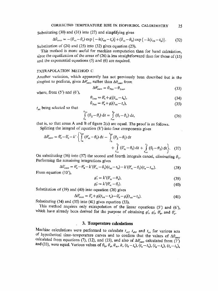
Substituting (30) and (31) into (27) and simplifying gives

A0 . . . . = - (0~ - 0~) exp ( - k(txb -- tc)} + ( 0 ~ -- Oh) exp { -- k(txb -- tb) }. (32)

Substitution of (24) and (25) into (32) gives equation (23). This method is more useful for machine computation than for hand calculation,

since the equalization of the areas of (26) is less straightforward than for those of (15) and the exponential equations (5) and (6) are required.

EXTRAPOLATION METHOD C

Another variation, which apparently has not previously been described but is the simplest to perform, gives A0'~orr rather than A0¢or~ from

A0'earr = 03x e - 01xe, where, from (5') and (6'),

Olxo = o; +o~(txo- tb), 03x¢ = 0'o + g~( t xo - t¢),

tx~ being selected so that

(33)

(34)

(35)

(36) txe te

S (02 - 0i) d t = j" ( 0 f - 02) dt, tb txe

that is, so that areas A and B of figure 2(c) are equal. The proof is as follows. Splitting the integral of equation (8') into four components gives

t~o txe ! ! # t #

A 0 . . . . = 0 e - - 0 b - k (0oo - - 0 i ) d t - ~ (02 - 01) d t L tb tb

te te t t + I (O'-Oe) d t + I (Oe-02) d . (37) txo txe

On substituting (36) into (37) the second and fourth integrals cancel, eliminating 02 . Performing the remaining integrations gives

. . . . 0 t ' ' A0"e,r = 0 e - 0 b - k (0~o - i) ( =c-- tb) -- k (0oo - Of) (t~ - tx~). (38) From equation (10'),

gl = k ' ( O " - Oi), (39)

g~ = k ' ( O " - 0f). (40) Substitution of (39) and (40) into equation (38) gives

a0'eorr = 0; --}- g~(txc-- t , ) - - O~,--g~(tx¢-- tb). (41) Substituting (34) and (35) into (41) gives equation (33).

This method requires only extrapolation of the linear equations (5') and (6'), which have already been derived for the purpose of obtaining g~., g~, 0k, and 0".

3. Temperature calculations

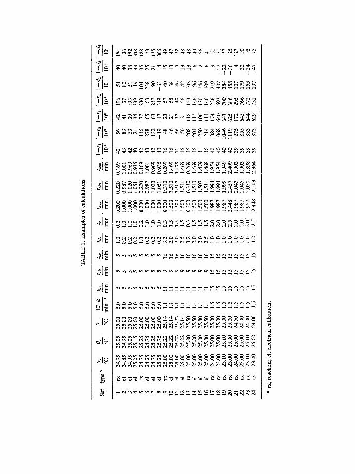
Machine calculations were performed to calculate txa , txb , and t~c for various sets of hypothetical time-temperature curves and to confirm that the values of A0 .... calculated from equations (7), (12), and (23), and also of A0'corr calculated from (7') and (33), were equal. Various values of 0b, 0¢, 0o~, k, (t b - ta) , ( t e - tb) , (t~-- to), (t s - tb) ~

0

o

S~

~ c

f7 I

C~

I l l I I

oo

o

o

CORRECTED TEMPERATURE RISE IN ISOPERIBOL CALORIMETRY 27

and tr were selected as shown in table 1. (In this table, the headings tba, teb, tze, t~b, txas, t~bs, and txc ~ are used to denote (tb-- t~), t~ -- tb), (tz -- t~), (t~ -- tb), (tx~ -- t~), (txS-- t~), and (txc-t~), respectively.) Points at 1 min intervals for the initial and final periods were calculated from equations (5) and (6). These points were then fitted by least squares to (5') and (6'). For the main periods, curves approximating typical electrical- heating calibrations and reactions were used; in table 1, these are designated "el" and "rx", respectively. For both, 02 was taken to be constant from t 5 to t~. The parameter (t~-ts) is introduced to approximate the fact that there may be some lag in reaching the maximum rate of temperature rise after initiation of reaction or electrical heating. Also, it may be desirable to delay initiation of reaction or electrical heating in order that (t~-ts) be similar for two measurements which are to be com- pared. However, t5 need not be the time at which 0 starts to diverge from equation (5); it may be any earlier time. Similarly t~ may be taken as any time after 0 is adequately close to the curve described by equation (6). For calibrations, Oz was taken to rise linearly from (t~, 05) to {(t~+2tr), 0o}, and then remain constant at 0o from (t~+2tr) to to; this gives t~ = t~ + tr. For reactions, 02 was considered to rise exponentially from (t~, 0b) to (t,, 0o) with a time constant t , according to the equation

02 = 0b + (0r-- 05) [1 -- exp {(t-- ts)ltr}], (42)

where 0 r is defined by

0r = 0b + (0o-- 05)/[-1 -- exp { -- (te-- ts)/tr}]. (43)

For (to-t~) >> tr, 0r = 0~ and tx, = (t~ + tr). All integrations were performed by a general procedure usable with curves of any

shape. The time interval was initially divided into 50 increments, the temperature value for each was calculated, and the area was integrated by the trapezoidal rule. The number of increments was then doubled and the integration performed again. This procedure was repeated until the results of successive integrations agreed within 0.001 per cent. For the extrapolation methods, t~ was initially set at (t5 + t~)/2 and the two areas defined by equation (15), (26), or (36) were integrated. Then t~ was increased or decreased in successive steps of ( t~- ts ) /4 , (te--tb)/8, (te--tb)/16, etc., until the two areas were equal within 0.01 per cent.

The agreement of A0 .... and A0'corr calculated by the various extrapolation methods with that calculated from equation (7) or (7') was exact in all cases. Table 1 gives the calculated extrapolation times for the three modifications for a range of con- ditions. While the differences between them are not gross, they are large enough to ensure that the extrapolation time obtained by the equalization of areas appropriate to one modification may lead to a significant error if used to extrapolate the curves appropriate to another modification.

Separate calculations of the differences (0b-0~) and (0~-0'e) were performed for various values of the thermal leakage modulus and period lengths. The results may be described by the equations:

Ob--O~ ~ k2(Ob--Ooo)( tb-- ta)( tb-- t , -At){O.O8333+O.O333k(tb- ta)+O.O17kAt} , (44) and

0~-0'o ~ k2(O~-Oo~)(tz- t~)( t - t -A t ){O.O8333-O.O333k( t - t e ) - O . O 1 7 k A t ) , (45)

28 S.R. GUNN

where At is the time interval between equally-spaced time-temperature points. These equations give values of the ratios (0~-0~)/(0b--0o~) and (0' e - 0o~)/(0o-0o0) correct within 12 p.p.m, for a thermal leakage modulus of 0.008 min -1 and a period length of 24 rain or a thermal leakage modulus of 0.016 min -1 and a period length of 12 min, and within 200 p.p.m, for a thermal leakage modulus of 0.016 rain -1 and a period length of 24 min or a thermal leakage modulus of 0.032 min- ~ and a period length of 12 min.

Table 1 includes values for the ratio:

r , = A0'~orr/A0corr. (46)

Neglecting higher-order terms in equations (44) and (45), and the difference between 50 and 80', we have

rl ~ l--(O.0833k2/AOcorr){(Oo~-Ob)(tb-ta)2-(Ooo-Oe)(tz-te)2}. (47)

For the case where (tb-- ta) = (tz-- re), and using the approximation A0 .... ~ (0~- 0b) , we have

rl ~ 1 - O.0833kz(tb-- ta) 2. (48)

It may be seen from this and the values for r~ in table 1 that variations of r 1 are quite negligible for a given calorimeter if the durations of the initial and final periods in the experiments being compared are approximately equal; thus A0'¢or~ is as valid as A0¢o~ as a measure of relative corrected temperature rises.

Coops, Jessup, and van Nes (2) pointed out that if the points of the initial or final periods are to be fitted to quadratic equations, it is preferable to calculate the coefficient of the second-order terms from preliminary values of k and gi or gf rather than to apply the method of least squares directly. Similarly, in fitting experi- mental results to the exponential equations (5) and (6) it may be desirable to use a value of k ' calculated from equation (9') with values of g~ and 9~ obtained from preliminary graphical or least-squares fits to equations (5') and (6'). Usually, k may be taken equal to k'. Where the durations of the periods are very large or the thermal leakage modulus is very large, the values of g'i and g~ may differ significantly from g~ and gf; approximate empirical relations are

gi ~ g;{1 + 0.0163k2(tb-- t. + 1.2At)2}, (49) and

gf ~ g~{1 + 0.0163k2(t~ - t~+ 1.2At)E}. (50)

which give ratios of gl/g~ and gf/g~ correct within 30 p.p.m, for a thermal leakage modulus of 0.016 rain -~ and a period length of 24 min or a thermal leakage modulus of 0.032 min- ~ and a period length of 12 min, and within 100 p.p.m. for a thermal leakage modulus of 0.032 min -1 and a period length of 24 min or a thermal leakage modulus of 0.064 min -1 and a period length of 12 min. Values of gi and gf from equations (49) and (50) may then be used in equation (9) to obtain an adequate value of k.

4. Change of steady power inputs to the calorimeter The most common cases wherein there is a change of the constant power input to the calorimeter are: (a) in solution calorimetry, where the breaking of a sample

CORRECTED TEMPERATURE RISE IN ISOPERIBOL CALORIMETRY 29

bulb at t b may change the heat of stirring, or a slow secondary reaction may start and continue at a nearly constant rate during the remainder of the run, and (b) in rotating-bomb combustion calorimetry, where a significant power is associated with rotation of the bomb, starting at a time ty, 1 or 2 rain after t b, and continuing to t~.

The present analysis does not apply to an alternate procedure wherein rotation is stopped before to. With the rotating-bomb combustion calorimeter, the increment A u (= Ap/e) due to rotation may be deduced by observing the drift rate gs of the calorimeter temperature with rotation at a mean temperature 0s and the drift rate gw without rotation at a mean temperature 0 w:

Au = g s - gw + k(Os- 0w). (51)

With the solution calorimeter, the changed stirring power may be detected as an abnormal value of k calculated from equation (9) or (9'). If a "normal" value of k is available (perhaps from electrical heating calibration experiments, wherein the stirring power does not change, with the same calorimeter setup), Au may be calculated from

Au = a e - {Oi- k(0f- 03}, (52)

where gf is the slope with changed stirring power in the final period. When calculating the corrected temperature rise the effect of Au may be eliminated

by various methods. Mathematically, these are all equivalent to the following:

0~, i = Oi "~ gl/k" (53)

O®,f = Of + g f /k = O~,i + Au/k . (54) ty te

A0oor, = eo-e -k J" (eoo, - d t - k I O2) dt. (55) tb ty

Good, Scott, and Waddington (8) pointed out that if ty is made to coincide with txa, then equations (12), (13), (14), and (15) give the correct value of A0 .... with the effect of Au eliminated. The same may be shown to be rigorously true for methods B and C if ty = t,b or ty = txc. However, in applying methods A and B rigorously, Au must be allowed for in the calculation of k and in fitting the initial and final periods. The value of k must be obtained not from equation (9) but rather from the following or an equivalent:

k = (gi - - Of-I- A u ) / ( 0 f - - 0i). (9a)

This value of k is needed for insertion in equations (5), (6), (21), (22), (24), and (25). In addition, 0~o,i must replace 0~ in (5) and (24), and 0o~,f must replace 0o~ in (6) and (25).

In method C no explicit allowance for Au is necessary; the actual initial and final periods may be fitted to the linear equations (5') and (6'), extrapolated to t~c according to (34) and (35), and applied to (33) to obtain the same value of A0'corr that would result from use of the integration method with (7'). However, if u (and hence 0o~) changes, the curvature of the final period will change and, from equation (46), (A0'¢orr-A0¢or~) will change; this may result in a small systematic error in the com-

30 s .R. GUNN

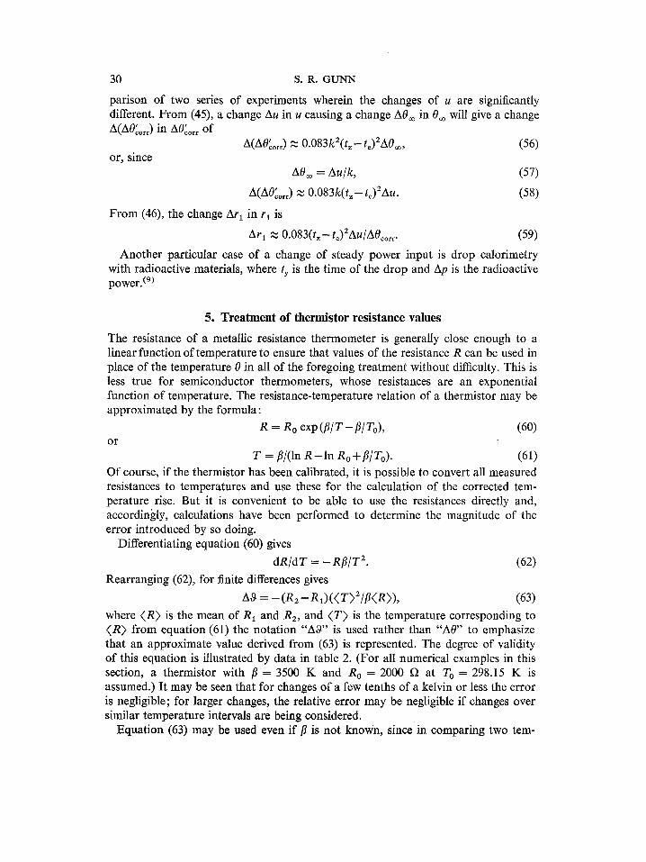
parison of two series of experiments wherein the changes of u are significantly different. From (45), a change Au in u causing a change A0~ in 0oo will give a change A(A0'corr) in A0rcorr of

A(A0'corr) g 0.083k2(tz - te)2A0®, (56) or, since

AO® = A u l k , (57)

A(A0;orr ) ,~ 0.083k(t z-/e)2Au. (58)

From (46), the change Ar 1 in r 1 is

Arl ~ 0.083(t~-to)2Au/A0 . . . . • (59)

Another particular case of a change of steady power input is drop calorimetry with radioactive materials, where ty is the time of the drop and Ap is the radioactive power. ° )

5. Treatment of thermistor resistance values

The resistance of a metallic resistance thermometer is generally close enough to a linear function of temperature to ensure that values of the resistance R can be used in place of the temperature 0 in all of the foregoing treatment without difficulty. This is less true for semiconductor thermometers, whose resistances are an exponential function of temperature. The resistance-temperature relation of a thermistor may be approximated by the formula:

R = R o exp ( f l / T - t~ To), (60) or

T = fl/(ln R - In n o + fl/To). (61) Of course, if the thermistor has been calibrated, it is possible to convert all measured resistances to temperatures and use these for the calculation of the corrected tem- perature rise. But it is convenient to be able to use the resistances directly and, accordingly, calculations have been performed to determine the magnitude of the error introduced by so doing.

Differentiating equation (60) gives

d n / d T = - R f l / T 2. (62)

Rearranging (62), for finite differences gives

A8 = - (R 2 - R 1) ( ( T ) 2 / f l ( R ) ) , (63)

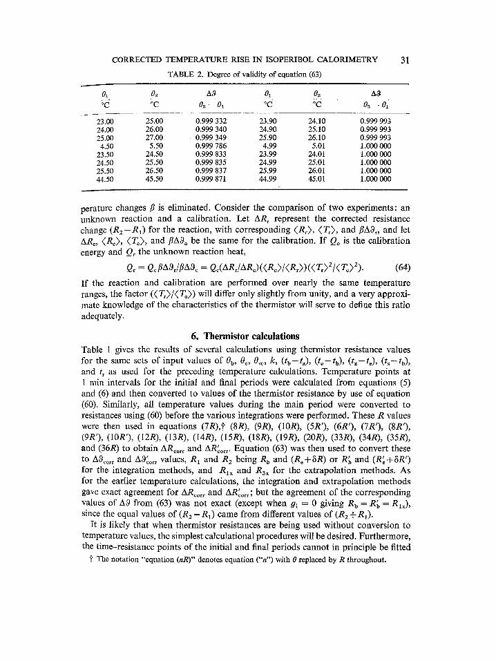
where ( R ) is the mean of R1 and R2, and ( T ) is the temperature corresponding to ( R ) from equation (61) the notation "A0" is used rather than "A0" to emphasize that an approximate value derived from (63) is represented. The degree of validity of this equation is illustrated by data in table 2. (For all numerical examples in this section, a thermistor with fi = 3500 K and R0 = 2000 f~ at To = 298.15 K is assumed.) It may be seen that for changes of a few tenths of a kelvin or less the error is negligible; for larger changes, the relative error may be negligible if changes over similar temperature intervals are being considered.

Equation (63) may be used even if fl is not known, since in comparing two tern-

CORRECTED TEMPERATURE RISE IN ISOPERIBOL CALORIMETRY

TABLE 2. Degree of validity of equation (63)

31

01 02 A0 0i 02 A0 °-6 ;~ 02 - 0~ oV o-~ o2 - 0~

23.00 25.00 0.999 332 23.90 24.10 0.999 993 24.00 26.00 0.999 340 24.90 25.10 0.999 993 25.00 27.00 0.999 349 25.90 26.10 0.999 993 4.50 5.50 0.999 786 4.99 5.01 1.000 000

23.50 24.50 0.999 833 23.99 24.01 1.000 000 24.50 25.50 0.999 835 24.99 25.01 1.000 000 25.50 26.50 0.999 837 25.99 26.01 1.000 000 44.50 45.50 0.999 871 44.99 45.01 1.000 000

perature changes fl is eliminated. Consider the comparison of two experiments: an unknown reaction and a calibration. Let ARr represent the corrected resistance change ( R 2 - R 0 for the reaction, with corresponding (Rr) , (T~), and flAOr, and let ARc, (Re), (To), and flA0c be the same for the calibration. I f Qc is the calibration energy and Qr the unknown reaction heat,

Qr = QcflAOrlflAOc = Qc(ARr lARc) ( (Rc) I (R , ) ) ( (T~)ZI (Tc)2) • (64)

If the reaction and calibration are performed over nearly the same temperature ranges, the factor ( ( T , ) / ( T c ) ) will differ only slightly from unity, and a very approxi- mate knowledge of the characteristics of the thermistor will serve to define this ratio adequately.

6. Thermistor calculations Table 1 gives the results of several calculations using thermistor resistance values for the same sets of input values of 0 b, 0 e, 0oo, k, (t b - t,), (t e - tb) , ( tz- te) , ( is-- tb) , and t~ as used for the preceding temperature calculations. Temperature points at 1 rain intervals for the initial and final periods were calculated from equations (5) and (6) and then converted to values of the thermistor resistance by use of equation (60). Similarly, all temperature values during the main period were converted to resistances using (60) before the various integrations were performed. These R values were then used in equations (7R),'~ (8R), (9R), (10R), (5R'), (6R'), (7R'), (8R'), (9R'), (10R'), (lZR), (13R), (14R), (15R), (lSR), (19R), (20R), (33R), (34R), (35R), and (36R) to obtain AR .... and AR'co,,. Equation (63) was then used to convert these to A0 .... and A0'corr values, R 1 and R2 being R b and (R e + 8R) or R~, and (R' e + 8R') for the integration methods, and Rlx and _R3x for the extrapolation methods. As for the earlier temperature calculations, the integration and extrapolation methods gave exact agreement for ARcor,- and AR'cor,; but the agreement of the corresponding values of A8 from (63) was not exact (except when Yi = 0 giving R b = R~, = Rlx), since the equal values of (R 2 - R 1 ) came from different values of (Rz + R O .

It is likely that when thermistor resistances are being used without conversion to temperature values, the simplest calculational procedures will be desired. Furthermore, the time-resistance points of the initial and final periods cannot in principle be fitted

• P The notation "equation (nR)" denotes equation ("n") with 0 replaced by R throughout.

32 S.R. GUNN

to equations (5R) and (6R), since temperature therein is an exponential function of time and resistance is in turn an exponential function of temperature. Accordingly, results are presented in table 1 only for methods involving linear approximations to the initial and final periods: the integration method, giving A8'c . . . . extrapolation method C, and a hybrid extrapolation method.

Extrapolation method C gives ASc, calculated by use of equation (63) with Rlx c and R3x~ from (34R) and (35R), txc being defined by (36R). However, it is often more convenient to equalize the areas according to extrapolation method A, using equation (15R) rather than (36R), and then to extrapolate (5R') and (6R') as in method C but to txa rather than the txo in (34R) and (35R). This is a hybrid method; the extra- polated values are designated R~xh and R3, h and inserted in (63) to obtain A8h.

The results of the three calculations are presented in table 1 as ratios to A0 .... •

r2 = A~'oorr/A0 .... . (65)

r 3 = A0¢/A0 .... • (66)

r4=AOh/A0 .... • (67)

Since A0 .... is obtained from an exact calculation (insofar as k, 0j, p, and e are constant), the error resulting from comparison of two experiments by the approxi- mate values A0'¢ .... AO'¢orr, AO¢, or AOa will be shown by comparing the values of r l , r2, r3, or r 4 for them. For example, consider the comparison of reaction 1 and calibration 3 using A0 n. The values of r 4 are 0.999 804 and 0.999 807; thus, a relative error of 3 p.p.m, results.

The permutations of the input parameters which might be of interest either in the temperature calculations or the thermistor resistance calculations are too numerous to present in this paper. Examples could be provided to show the influence of changes in each parameter while all other parameters are kept constant at various values. Table 1 includes examples for only three general ranges of conditions.

Sets 1 to 8 represent conditions that might obtain with a small solution or reaction calorimeter. Comparisons of set 1 with set 3 and set 5 with set 7 show that the errors for the approximate methods are small when the calibration and reaction cover the same temperature interval. But when the calibrations are over different temperature intervals (compare set 1 with set 2 or set 4), the errors for some methods increase considerably, and are still larger for larger temperature rises (compare set 5 with set 6 or set 8).

Sets 9, 10, 13, and 14 represent conditions for a recent high precision solution- calorimetric investigation. (1°) Here A~ h was used; the values of r4 show resulting errors of only 3 and 9 p.p.m, when conditions were well matched. Changing 0o0 from {0~-0.4(0c-0b)} to 0 e gives a change of only 15 p.p.m, in r4 (compare set 11 with set 10, and set 15 with set 14). Changing t s by 0.5 min gives no change (compare set 12 with set 10, and set 16 with set 14).

Sets 17 to 24 represent conditions that might obtain with a combustion calorimeter. For sets 17 to 20, the convergence temperature is equal to or near the final tempera- ture; for sets 21 to 24, it is equal to or near the mean temperature. It may be seen that r3 and r 4 change little when 0b and 0o are both increased by 0.1 °C (compare

CORRECTED TEMPERATURE RISE IN ISOPERIBOL CALORIMETRY 33

set 19 with set 18, and set 23 with set 22) or when the kinetics of the reaction change (tr 0.5 rain greater, compare set 20 with set 18, or set 24 with set 22), but that r2, r3, and r4 are all considerably different for 1 °C and 2 °C rises (compare set 17 with set 18, or set 21 with set 22).

This variation of r with the magnitude of the temperature rise is largely due to the approximate nature of equation (63), as illustrated by table 2. This effect may be eliminated by an alternate procedure: when the two values R t and R 2 a r e obtained, instead of being inserted together into (63), they are inserted individually into equa- tion (61). This requires only two conversions of R to T by use of (61); the advantages of using R directly in the rest of the calculation are retained. Using T(R) to denote a value of 0 calculated from a particialar value of R by (61), we may define

d2 = {T(R'~ + 5R) - T(R~,)}/AOcor, :. (68)

d3 = {T(Raxc)- T(RI,,c))/AO . . . . • (69)

d4 = {T(Raxh)- T(Raxh)}/AO . . . . • (70)

Thus d2, da, and d 4 correspond to r2, r3, and r 4 with the approximation due to (63) removed; these are tabulated in the last three columns of table 1. It may be seen, for the comparison of substantially different temperature rises, that this treatment is considerably superior (compare set 17 with set 18, and set 21 with set 22).

In some cases the values of k and 0o~ calculated from equations (9R'), (10R'), and (61) differ substantially from the true (input) values even when ratios of AO'c .... A0~, or A0h are quite satisfactory for comparison of experiments. Thus for sets 17 and 18 the calculated values of k are 0.001 535 and 0.001 572, respectively.

In general, the validity of using any of the approximate methods in comparing two experiments is increased when for the two experiments the following desiderata are approached: (a) the value of A0 .... is small; (b) the values of (tb--ta) , (t~--tb) , (tz--to), and k are equal and small; (c) the values of 0b, 05, and 0~o are equal; (d) the shapes of 02 against t (temperature during the main period) are similar, giving equal values of (t x - tb).

A F O R T R A N program is available from the author or from ASIS-NAPS for persons wishing to repeat these calculations at particular conditions of interest to themselves (see reference 11).

REFERENCES

1. Dickinson, H. C. Bull. Nat. Bur. Std. (U.S.) 1914, 11, 189. 2. Coops, J. ; Jessup, R. S.; van Nes, K. Calibrations of calorimeters for reactions in a bomb at

constant volume, Chap. 3 in Experimental Thermochemistry. Rossini, F. D.; editor. Interscience: New York. 1956.

3. ChaIloner, A. R. ; Gundry, H. A. ; Meetham, A. R. Phil. Trans. Roy. Soc. Lond. 1955, A247, 553. 4. King, A.; Grover, H. J. AppL Phys. 1941, 12, 557. 5. Jessup, R. S. J. Appl. Phys. 1942, 13, 128. 6. Macleod, A. C. Trans. Faraday Soc. 1967, 63, 289. 7. West, E. D.; Churney, K. L. J. Appl. Phys. 1968, 39, 4206. 3

34 S . R . GUNN

8. Good, W. D.; Scott, D. W.; Waddington, G. d. Phys. Chem. 1956, 60, 1080. 9. Oetting, F. L. d. Chem. Thermodynamics 1970, 2, 727.

10. Gunn, S. R. J. Chem. Thermodynamics 1970, 2, 535. 11. For a copy of this FORTRAN program order NAPS Document 01179 from ASIS National

Auxiliary Publications Service c/o CCM Information Sciences, Inc., 909 Third Avenue, New York, N.Y. 10022, remitting $2.00 for microfiche or $5.00 for photocopies.