ON THE COMPLEXITY OF COMPUTING DETERMINANTSperso.ens-lyon.fr/gilles.villard/BIBLIOGRAPHIE/PDF/KaVi04.pdf · polynomial is the characteristic polynomial, and the determinants of the

comput. complex. 13 (2004), 91 – 130

1016-3328/04/030091–40

DOI 10.1007/s00037-004-0185-3

c© Birkhauser Verlag, Basel 2004

computational complexity

ON THE COMPLEXITY OF COMPUTING

DETERMINANTS

Erich Kaltofen and Gilles Villard

To B. David Saunderson the occasion of his 60th birthday

Abstract. We present new baby steps/giant steps algorithms ofasymptotically fast running time for dense matrix problems. Our al-gorithms compute the determinant, characteristic polynomial, Frobe-nius normal form and Smith normal form of a dense n × n matrix Awith integer entries in (n3.2 log ‖A‖)1+o(1) and (n2.697263 log ‖A‖)1+o(1)

bit operations; here ‖A‖ denotes the largest entry in absolute valueand the exponent adjustment by “+o(1)” captures additional factorsC1(log n)C2(loglog ‖A‖)C3 for positive real constants C1, C2, C3. Thebit complexity (n3.2 log ‖A‖)1+o(1) results from using the classical cubicmatrix multiplication algorithm. Our algorithms are randomized, andwe can certify that the output is the determinant of A in a Las Vegasfashion. The second category of problems deals with the setting wherethe matrix A has elements from an abstract commutative ring, that is,when no divisions in the domain of entries are possible. We presentalgorithms that deterministically compute the determinant, character-istic polynomial and adjoint of A with n3.2+o(1) and O(n2.697263) ringadditions, subtractions and multiplications.

Keywords. Integer matrix, matrix determinant, characteristic poly-nomial, Smith normal form, bit complexity, division-free complexity,randomized algorithm, multivariable control theory, realization, matrixsequence, block Wiedemann algorithm, block Lanczos algorithm.

Subject classification. 68W30, 15A35.

1. Introduction

The computational complexity of many problems in linear algebra has beentied to the computational complexity of matrix multiplication. If the resultis to be exact, for example the exact rational solution of a linear system, thelengths of the integers involved in the computation and the answer affect the

92 Kaltofen & Villard cc 13 (2004)

running time of the used algorithms. A classical methodology is to computethe results via Chinese remaindering. Then the standard analysis yields anumber of fixed radix, i.e. bit operations for a given problem that is essentially(within polylogarithmic factors) bounded by the number of field operations forthe problem times the maximal scalar length in the output. The algorithmsat times use randomization, because not all modular images may be usable.For the determinant of an n × n integer matrix A one thus gets a runningtime of (n4 log ‖A‖)1+o(1) bit operations (von zur Gathen & Gerhard 1999,Chapter 5.5), because the determinant can have at most (n log ‖A‖)1+o(1) digits;by ‖A‖ we denote the largest entry in absolute value. Here and throughoutthis paper the exponent adjustment by “+o(1)” captures additional factorsC1(log n)C2(loglog ‖A‖)C3 for positive real constants C1, C2, C3 (“soft-O”). Viaan algorithm that can multiply two n×n matrices inO(nω) scalar operations thetime is reduced to (nω+1 log ‖A‖)1+o(1). We can set ω = 2.375477 (Coppersmith& Winograd 1990).

First, it was recognized that for the problem of computing the exact rationalsolution of a linear system the process of Hensel lifting can accelerate the bitcomplexity beyond the Chinese remainder approach (Dixon 1982), namely tocubic in n without using fast matrix multiplication algorithms. For the deter-minant of an n × n integer matrix A, an algorithm with (n3.5 log ‖A‖1.5)1+o(1)

bit operations is given by Eberly et al. (2000).1 Their algorithm computes theSmith normal form via the binary search technique of Villard (2000).

Our algorithms combine three ideas.

(i) The first is an algorithm by Wiedemann (1986) for computing the deter-minant of a sparse matrix over a finite field. Wiedemann finds the mini-mum polynomial for the matrix as a linear recurrence on a correspondingKrylov sequence. By preconditioning the input matrix, that minimumpolynomial is the characteristic polynomial, and the determinants of theoriginal and preconditioned matrix have a direct relation.

(ii) The second is by Kaltofen (1992) where Wiedemann’s approach is appliedto dense matrices whose entries are polynomials over a field. Kaltofenachieves speedup by employing Shank’s baby steps/giant steps techniquefor the computation of the linearly recurrent scalars (cf. Paterson & Stock-meyer 1973). For integer matrices the resulting randomized algorithm isof the Las Vegas kind—always correct, probably fast—and has worst case

1Eberly et al. (2000) give an exponent for log ‖A‖ of 2.5, but the improvement to 1.5based on fast Chinese remaindering (Aho et al. 1974) is immediate.

cc 13 (2004) Complexity of computing determinants 93

bit complexity (n3.5 log ‖A‖)1+o(1) and again can be speeded with sub-cubic time matrix multiplication (Kaltofen & Villard 2001). A detaileddescription of this algorithm, with an early termination strategy in casethe determinant is small (cf. Bronnimann et al. 1999; Emiris 1998), ispresented by Kaltofen (2002).

(iii) By considering a bilinear map using two blocks of vectors rather than asingle pair of vectors, Wiedemann’s algorithm can be accelerated (Copper-smith 1994; Kaltofen 1995; Villard 1997a,b). Blocking can be applied toour algorithms for dense matrices and further reduces the bit complexity.

The above ingredients yield a randomized algorithm of the Las Vegas kindfor computing the determinant of an n × n integral matrix A in (n3+1/3×log ‖A‖)1+o(1) expected bit operations, that with a standard cubic matrix mul-tiplication algorithm. If we employ fast FFT-based Pade approximation algo-rithms for matrix polynomials, for example the so-called half-GCD algorithm(von zur Gathen & Gerhard 1999) and fast matrix multiplication algorithms,we can further lower the expected number of bit operations. Under the as-sumption that two n×n matrices can be multiplied in O(nω) operations in thefield of entries, and an n× n matrix by an n× nζ matrix in n2+o(1) operations,we obtain an expected bit complexity for the determinant of

(1.1) (nη log ‖A‖)1+o(1) with η = ω +1− ζ

ω2 − (2 + ζ)ω + 2.

The best known values ω = 2.375477 (Coppersmith & Winograd 1990) andζ = 0.2946289 (Coppersmith 1997) yield η = 2.697263. For ω = 3 and ζ = 0we have η = 3 + 1/5 as given in the abstract above.

Our techniques can be further combined with the ideas by Giesbrecht (2001)to produce a randomized algorithm for computing the integer Smith normalform of an integer matrix. The method becomes Monte Carlo—always fastand probably correct—and has the same bit complexity (1.1). In addition,we can compute the characteristic polynomial of an integer matrix by Hensellifting (Storjohann 2000b). Again the method is Monte Carlo and has bitcomplexity (1.1). Both results utilize the fast determinant algorithm for matrixpolynomials (Storjohann 2002, 2003).

The algorithm by Kaltofen (1992) (see case ii above) was originally put toa different use, namely that of computing the characteristic polynomial andadjoint of a matrix without divisions, counting additions, subtractions, andmultiplications in the commutative ring of entries. Serendipitously, blocking(see case iii above) can be applied to our original 1992 division-free algorithm,


and we obtain a deterministic algorithm that computes the determinant andcharacteristic polynomial of a matrix over a commutative ring in nη+o(1) ringadditions, subtractions and divisions, where η is given by (1.1). The exponentη = 2.697263 seems to be the best that is known today for the division-freedeterminant problem. By the technique of Baur and Strassen (1983) we obtainthe adjoint of a matrix in the same division-free complexity.

Kaltofen and Villard (2004) have identified other algorithms for computingthe determinant of an integer matrix. Those algorithms often perform at cubicbit complexity on what we call propitious inputs, but they have a worst casebit complexity that is higher than our methods. One such method is Clarkson’salgorithm (Bronnimann & Yvinec 2000; Clarkson 1992), where the number ofmantissa bits in the intermediate floating point scalars that are necessary forobtaining a correct sign depends on the orthogonal defect of the matrix. If thematrix has a large first invariant factor, Chinese remaindering can be employedin connection with computing the solution of a random linear system via Hensellifting (Abbott et al. 1999; Pan 1988).

Notation. By Sm×n we denote the set of m × n matrices with entries in theset S. The set Z are the integers. For A ∈ Zn×n we denote by ‖A‖ the matrixheight (Kaltofen & May 2003, Lemma 2):

‖A‖ = ‖A‖∞,1 = maxx6=0‖Ax‖∞/‖x‖1 = max

1≤i,j≤n|ai,j|.

Hence the maximal bit length of all entries in A and their signs is, dependingon the exact representation, at least 2 + blog2 max{1, ‖A‖}c. In order to avoidzero factors or undefined logarithms, we shall simply define ‖A‖ > 1 wheneverit is necessary.

Organization of the paper. Section 2 introduces Coppersmith’s block Wiede-mann algorithm and establishes all necessary mathematical properties of thecomputed matrix generators. In particular, we show the relation of the de-terminants of the generators with the (polynomial) invariant factors of thecharacteristic matrix (Theorem 2.12), which essentially captures the block ver-sion of the Cayley–Hamilton property. In addition, we characterize when shortsequences are insufficient to determine the minimum generator. Section 3 dealswith the computation of the block generator. We give the generalization ofthe Knuth/Schonhage/Moenck algorithm for polynomial quotient sequences tomatrix polynomials and show that in our case by randomization all leadingcoefficients stay non-singular (Lemma 3.10). Section 4 presents our new de-terminant algorithm for integer matrices and gives the running time analysis


when cubic matrix multiplication algorithms are employed (Theorem 4.2). Sec-tion 5 presents the division-free determinant algorithm. Section 6 contains theanalysis for versions of our algorithms when fast matrix multiplication is intro-duced. The asymptotically best results are derived there. Section 7 presentsthe algorithms for the Smith normal form and the characteristic polynomial ofan integer matrix. We give concluding thoughts in Section 8.

2. Generating polynomials of matrix sequences

Coppersmith (1994) first introduced blocking to the Wiedemann method. Inour description we also take into account the interpretation by Villard (1997a;1997b), where the relevant literature from linear control theory is cited. Ouralgorithms rely on the notion of minimum linear generating polynomials (gen-erators) of matrix sequences. This notion is introduced below in Section 2.1.We also see how generators are related to block Hankel matrices and recallsome basic facts concerning their computation. In Section 2.2 we then studydeterminants and Smith normal forms of generators and see how they will beused for solving our initial problem. All the results are given over an arbitrarycommutative field K.

2.1. Generators and block Hankel matrices. For the “block” vectorsX ∈ Kn×l and Y ∈ Kn×m consider the sequence of l ×m matrices

(2.1) B[0] = XTrY, B[1] = XTrAY, B[2] = XTrA2Y, . . . , B[i] = XTrAiY, . . .

As in the unblocked Wiedemann method, we seek linear generating polyno-mials. A vector polynomial

∑di=0 c

[i]λi, where c[i] ∈ Km, is said to linearlygenerate the sequence (2.1) from the right if

(2.2) ∀j ≥ 0:

d∑

i=0

B[j+i]c[i] =

d∑

i=0

XTrAi+jY c[i] = 0l.

For the minimum polynomial of A, fA(λ), and for the µ-th unit vector in Km,e[µ], fA(λ)e[µ] ∈ K[λ]m is such a generator because it already generates theKrylov sequence {AiY [µ]}i≥0, where Y [µ] is the µ-th column of Y . We can nowconsider the set of all such right vector generators. This set forms a K[λ]-submodule of the K[λ]-module K[λ]m and contains m linearly independent(over the field of rational functions K(λ)) elements, namely all fA(λ)e[µ]. Fur-thermore, the submodule has an (“integral”) basis over K[λ], namely any set ofm linearly independent generators such that the degree in λ of the determinant


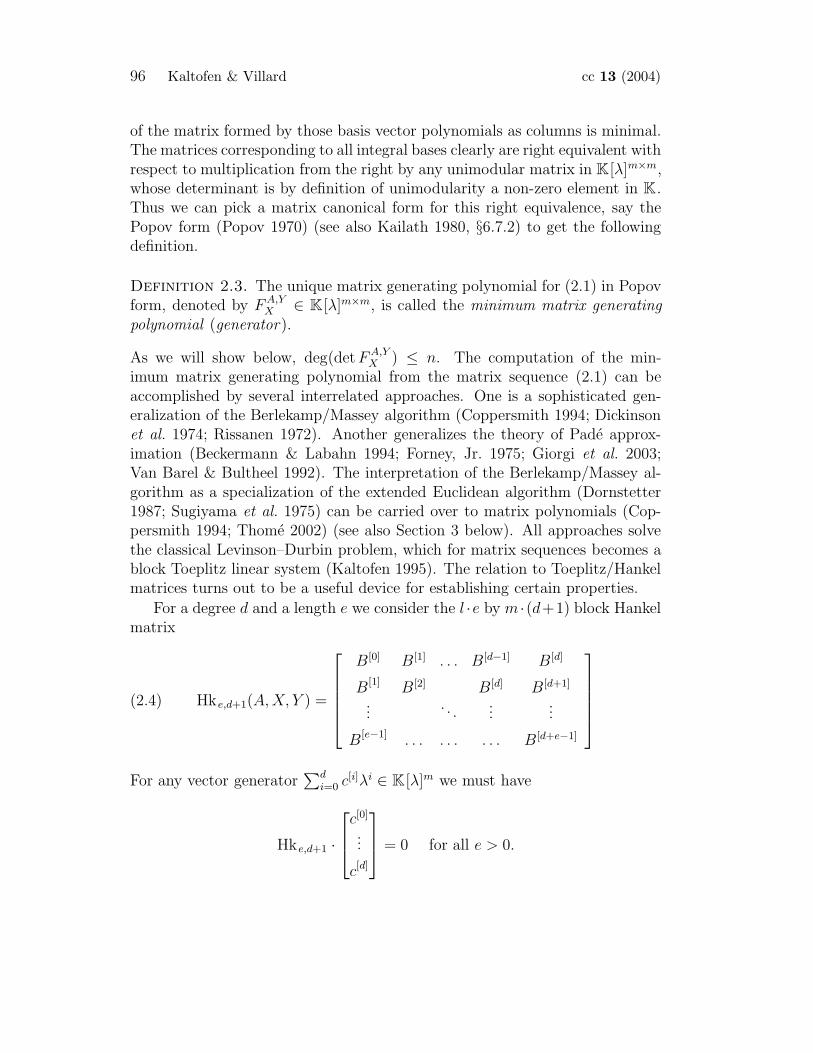
of the matrix formed by those basis vector polynomials as columns is minimal.The matrices corresponding to all integral bases clearly are right equivalent withrespect to multiplication from the right by any unimodular matrix in K[λ]m×m,whose determinant is by definition of unimodularity a non-zero element in K.Thus we can pick a matrix canonical form for this right equivalence, say thePopov form (Popov 1970) (see also Kailath 1980, §6.7.2) to get the followingdefinition.

Definition 2.3. The unique matrix generating polynomial for (2.1) in Popovform, denoted by FA,Y

X ∈ K[λ]m×m, is called the minimum matrix generatingpolynomial (generator).

As we will show below, deg(detFA,YX ) ≤ n. The computation of the min-

imum matrix generating polynomial from the matrix sequence (2.1) can beaccomplished by several interrelated approaches. One is a sophisticated gen-eralization of the Berlekamp/Massey algorithm (Coppersmith 1994; Dickinsonet al. 1974; Rissanen 1972). Another generalizes the theory of Pade approx-imation (Beckermann & Labahn 1994; Forney, Jr. 1975; Giorgi et al. 2003;Van Barel & Bultheel 1992). The interpretation of the Berlekamp/Massey al-gorithm as a specialization of the extended Euclidean algorithm (Dornstetter1987; Sugiyama et al. 1975) can be carried over to matrix polynomials (Cop-persmith 1994; Thome 2002) (see also Section 3 below). All approaches solvethe classical Levinson–Durbin problem, which for matrix sequences becomes ablock Toeplitz linear system (Kaltofen 1995). The relation to Toeplitz/Hankelmatrices turns out to be a useful device for establishing certain properties.

For a degree d and a length e we consider the l ·e by m ·(d+1) block Hankelmatrix

(2.4) Hke,d+1(A,X, Y ) =

B[0] B[1] . . . B[d−1] B[d]

B[1] B[2] B[d] B[d+1]

.... . .

......

B[e−1] . . . . . . . . . B[d+e−1]

For any vector generator∑d

i=0 c[i]λi ∈ K[λ]m we must have

Hke,d+1 ·

c[0]

...

c[d]

= 0 for all e > 0.


By considering the rank of (2.4) we can infer the reverse. If

(2.5) Hkn,d+1 ·

c[0]

...

c[d]

= 0

then∑d

i=0 c[i]λi is a vector generator of (2.1). The claim follows from the fact

that rank Hkn,d+1 = rank Hkn+e′,d+1 for all e′ > 0. The latter is justified byobserving that any row in the (n + e′)th block row of Hkn+e′,d+1 is linearlydependent on corresponding previous rows via the minimum polynomial fA,which has degree deg fA ≤ n.

We observe that rank Hke,d ≤ n for all d > 0, e > 0 by considering thefactorization

Hke,d =

XTr

XTrAXTrA2

...XTrAe−1

·[Y AY A2Y . . . Ad−1Y

]

and noting that either matrix factor has rank at most n.

Therefore, when d ≥ deg FA,YX , the module over K[λ] generated by solutions

to (2.5) is the module of vector generators, with the columns of F A,YX (λ) as

basis. In this case, if the column degrees of the minimum generator are δ1 ≤· · · ≤ δm, the dimension of the right nullspace of Hk e,d+1 in (2.5) over K is

(d− δ1 + 1) + · · ·+ (d − δm + 1). Hence for d ≥ degFA,YX and e ≥ n we have

rank Hke,d+1 = δ1 + · · ·+ δm = deg(detFA,YX ) ≤ n, the latter because FA,Y

X (λ)

is in Popov form. Since the last block column in Hk e,d+1 with d ≥ deg FA,YX

is generated by previous block columns, via shifting lower degree columns ofFA,YX (λ) as necessary by multiplying with powers of λ, we have

(2.6) rank Hke,d = deg(detFA,YX ) for d ≥ deg FA,Y

X and e ≥ n.

One may now define the minimum emin such that the matrix Hkemin,d for

d = degFA,YX has full rank deg(detFA,Y

X ). Any algorithm for computingthe minimum generator requires the first degFA,Y

X + emin elements of the se-quence (2.1).


We give an example over Q (Turner 2002). Let

A =

0 1 0 00 0 1 00 0 0 12 0 0 0

, X = Y =

1 00 00 00 0

Then

B[0] =

[1 00 0

], B[1] =

[0 00 0

], B[2] =

[0 00 0

], B[3] =

[0 00 0

],

B[4] =

[2 00 0

], B[5] =

[0 00 0

], B[6] =

[0 00 0

], B[7] =

[0 00 0

].

Therefore

Hk4,5(A,X, Y ) =

1 0 0 0 0 0 0 0 2 00 0 0 0 0 0 0 0 0 00 0 0 0 0 0 2 0 0 00 0 0 0 0 0 0 0 0 00 0 0 0 2 0 0 0 0 00 0 0 0 0 0 0 0 0 00 0 2 0 0 0 0 0 0 00 0 0 0 0 0 0 0 0 0

,

and since the nullspace of Hk4,5(A,X, Y ) is generated by the vectors

−2000000010

,

0100000000

,

0001000000

,

0000010000

,

0000000100

,

0000000001

,

we get

FA,YX (λ) =

[1 00 0

]λ4 +

[−2 00 1

]=

[λ4 − 2 0

0 1

].


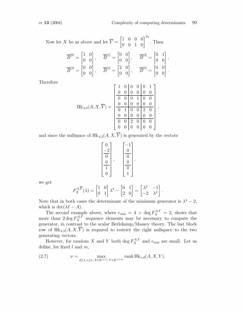
Now let X be as above and let Y =

[1 0 0 00 0 1 0

]Tr

. Then

B[0]

=

[1 00 0

], B

[1]=

[0 00 0

], B

[2]=

[0 10 0

],

B[3]

=

[0 00 0

], B

[4]=

[2 00 0

], B

[5]=

[0 00 0

].

Therefore

Hk4,3(A,X, Y ) =

1 0 0 0 0 10 0 0 0 0 00 0 0 1 0 00 0 0 0 0 00 1 0 0 2 00 0 0 0 0 00 0 2 0 0 00 0 0 0 0 0

,

and since the nullspace of Hk4,3(A,X, Y ) is generated by the vectors

0−20010

,

−100001

,

we get

FA,YX (λ) =

[1 00 1

]λ2 −

[0 12 0

]=

[λ2 −1−2 λ2

].

Note that in both cases the determinant of the minimum generator is λ4 − 2,which is det(λI − A).

The second example above, where emin = 4 > degFA,YX = 2, shows that

more than 2 degFA,YX sequence elements may be necessary to compute the

generator, in contrast to the scalar Berlekamp/Massey theory. The last blockrow of Hk4,3(A,X, Y ) is required to restrict the right nullspace to the twogenerating vectors.

However, for random X and Y both degFA,YX and emin are small. Let us

define, for fixed l and m,

(2.7) ν = maxd≥1, e≥1, X∈Kn×l, Y ∈Kn×m

rank Hke,d(A,X, Y ).


Indeed, the probabilistic analysis in (Kaltofen 1995, Section 5) and (Villard1997b, Corollary 6.4) shows the existence of matrices W ∈ Kn×l and Z ∈ Kn×m

such that rank Hke0,d0(A,W,Z) = ν with d0 = dν/me and e0 = dν/le. More-over, ν is equal to the sum of the degrees of the first min{l, m} invariant factorsof λI − A (see Theorem 2.12 below), and hence X, Y can be taken from anyfield extension of K. Then due to the existence of W,Z, for symbolic entries inX, Y and therefore, by (DeMillo & Lipton 1978; Schwartz 1980; Zippel 1979),for random entries, the maximal rank is preserved for block dimensions e0, d0.Note that the degree of the minimum matrix generating polynomial is nowdegFA,Y

X = d0 < n/m + 1 and the number of sequence elements required tocompute the minimum generator is d0 + e0 = dν/le + dν/me < n/l + n/m + 2.If K is a small finite field, Wiedemann’s analysis has been generalized by Vil-lard (1997b) (see also Brent et al. 2003).

As with the unblocked Wiedemann projections, unlucky projection blockvectors X and Y may cause a drop in the determinantal degree deg(detF A,Y

X ).They may also increase the length of the sequence required to compute thegenerator FA,Y

X .

2.2. Smith normal forms of matrix generating polynomials. In thissection we study how the invariant structure of FA,Y

X partly reveals the structureof A and λI−A. Our algorithms in Sections 4 and 5 pick random block vectorsX, Y or use special projections and compute a generator from the first d0 + e0

elements of (2.1). Under the assumption that rank Hk e,d = ν (see (2.7)) for

sufficiently large d, e, we prove here that detFA,YX is the product of the first

min{l, m} invariant factors of λI−A. These are well-studied facts in the theoryof realizations of multivariable control theory; for instance see Kailath (1980).The basis is the matrix power series

XTr(λI − A)−1Y = XTr

(∑

i≥0

Ai

λi+1

)Y =

∑

i≥0

B[i]

λi+1.

Lemma 2.8. One has the fraction description

(2.9) XTr(λI − A)−1Y = N(λ)D(λ)−1

if and only if there exists T ∈ K[λ]m×m such that D = FA,YX T .

Proof. For the necessary condition, since every polynomial numerator inXTr(λI − A)−1Y has degree strictly less than the corresponding denominator,


every column of N has degree strictly less than that of the corresponding col-umn of D. Thus it can be checked that the columns of D satisfy (2.2) andD must be a multiple of FA,Y

X . Conversely, let D = FA,YX T in K[λ]m×m be an

invertible matrix generator for (2.1). Using (2.2) for its m columns it can beseen that we have

XTr(λI − A)−1Y D(λ) = N(λ) ∈ K[λ]l×m,

where the column degrees of N are lower than those of D. This yields thematrix fraction description (2.9). �

Clearly, for D = FA,YX , the minimum polynomial fA(λ) is a common de-

nominator of the rational entries of the matrices on both sides of (2.9). If theleast common denominator of the left side matrix is actually the character-istic polynomial det(λI − A), then it follows from degree considerations thatdetFA,Y

X = det(λI − A). Our algorithm uses the matrix preconditioners dis-cussed in Section 4 and random or ad hoc projections (Section 5) to achievethis determinantal equality. We shall make the relationship between λI − Aand FA,Y

X more explicit in Theorem 2.12 whose proof will rely on the structureof the matrix denominator D in (2.9) and on the following.

For a square matrix M over K[λ] we consider the Smith normal form (New-man 1972), which is an equivalent diagonal matrix over K[λ] with diagonalelements s1(λ), . . . , sφ(λ), 1, . . . , 1, 0, . . . , 0, where the si’s are the non-trivialinvariant factors of M , that is, non-constant monic polynomials with the prop-erty that si is a (trivial or nontrivial) polynomial factor of si−1 for all 2 ≤ i ≤ φ.Because the Smith normal form of the characteristic matrix λI−A correspondsto the Frobenius canonical form of A for similarity, the largest invariant factorof λI − A, s1(λ), equals the minimum polynomial fA(λ).

Lemma 2.10. Let M ∈ K[λ]µ×µ be non-singular and let U ∈ K[λ]µ×µ beunimodular such that

(2.11) MU =

[H H12

0 H22

],

where H is a square matrix. Then the i-th invariant factor of H divides thei-th invariant factor of M .

Proof. Identity (2.11) may be rewritten as

MU =

[I H12

0 H22

] [H 00 I

].


Since the invariant factors of two non-singular matrices divide the invariantfactors of their product (Newman 1972, Theorem II.14), the largest invariantfactors of diag(H, I) that are those of H, divide the corresponding invariantfactors of MU and thus M . �

We can now see how the Smith form of FA,YX is related to that of λI − A.

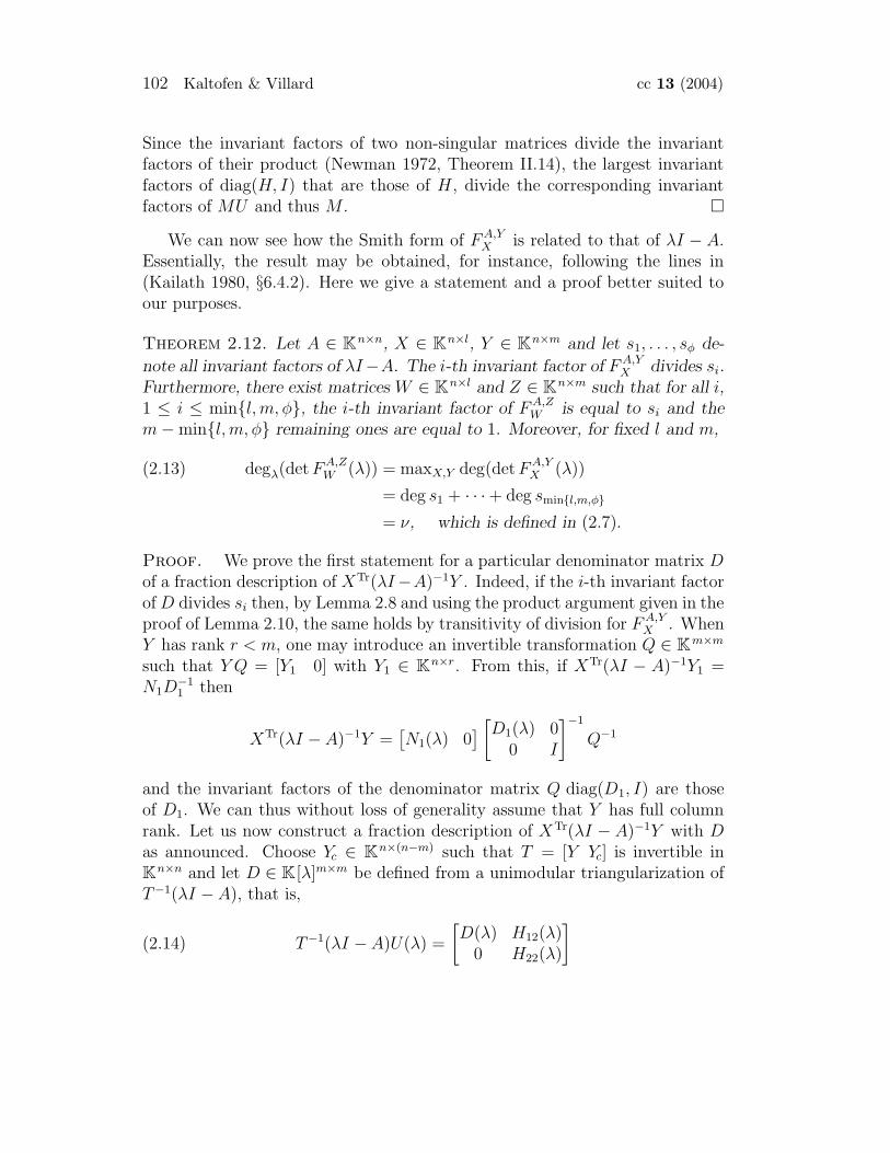
Essentially, the result may be obtained, for instance, following the lines in(Kailath 1980, §6.4.2). Here we give a statement and a proof better suited toour purposes.

Theorem 2.12. Let A ∈ Kn×n, X ∈ Kn×l, Y ∈ Kn×m and let s1, . . . , sφ de-

note all invariant factors of λI−A. The i-th invariant factor of F A,YX divides si.

Furthermore, there exist matrices W ∈ Kn×l and Z ∈ Kn×m such that for all i,1 ≤ i ≤ min{l, m, φ}, the i-th invariant factor of FA,Z

W is equal to si and them−min{l, m, φ} remaining ones are equal to 1. Moreover, for fixed l and m,

(2.13) degλ(detFA,ZW (λ)) = maxX,Y deg(detFA,Y

X (λ))

= deg s1 + · · ·+ deg smin{l,m,φ}

= ν, which is defined in (2.7).

Proof. We prove the first statement for a particular denominator matrix Dof a fraction description of XTr(λI−A)−1Y . Indeed, if the i-th invariant factorof D divides si then, by Lemma 2.8 and using the product argument given in theproof of Lemma 2.10, the same holds by transitivity of division for F A,Y

X . WhenY has rank r < m, one may introduce an invertible transformation Q ∈ Km×m

such that Y Q = [Y1 0] with Y1 ∈ Kn×r. From this, if XTr(λI − A)−1Y1 =N1D

−11 then

XTr(λI − A)−1Y =[N1(λ) 0

] [D1(λ) 00 I

]−1

Q−1

and the invariant factors of the denominator matrix Q diag(D1, I) are thoseof D1. We can thus without loss of generality assume that Y has full columnrank. Let us now construct a fraction description of XTr(λI − A)−1Y with Das announced. Choose Yc ∈ Kn×(n−m) such that T = [Y Yc] is invertible inKn×n and let D ∈ K[λ]m×m be defined from a unimodular triangularization ofT−1(λI − A), that is,

(2.14) T−1(λI − A)U(λ) =

[D(λ) H12(λ)

0 H22(λ)

]


with U unimodular. If V is the matrix formed by the first m columns of U wehave the fraction descriptions (λI − A)−1Y = V D−1 and XTr(λI − A)−1Y =(XTrV )D−1. Thus D is a denominator matrix for XTr(λI − A)−1Y . By (2.14)and Lemma 2.10, its i-th invariant factor divides the i-th invariant factor si ofλI − A and the first assertion is proven.

To establish the rest of the theorem we work with the associated blockHankel matrix Hke,d(A,X, Y ). By definition of the invariant factors we knowthat

dim span(X,ATrX, (ATr)2X, . . .) ≤ deg s1 + · · ·+ deg smin{l,φ}

anddim span(Y,AY,A2Y, . . .) ≤ deg s1 + · · ·+ deg smin{m,φ},

thus

rank Hke,d(A,X, Y ) ≤ rank

XTr

XTrAXTrA2

...

·[Y AY A2Y . . .

]

≤ ν,

where ν = deg s1 + · · ·+ deg smin{m,l,φ}. Hence, from the specializations W andZ of X and Y given in (Villard 1997b, Corollary 6.4), we get

(2.15) rank Hke0,d0(A,W,Z) = maxX,Y,d,e

rank Hke,d+1(A,X, Y ) = ν

with d0 = dν/me and e0 = dν/le and thus ν = ν. Using (2.6) we also have

(2.16) degλ(detFA,ZW (λ)) = max

X,Ydegλ(detFA,Y

X (λ)) = ν.

With (2.15) and (2.16) we have proven the two maximality assertions. Inaddition, since the i-th invariant factor si of FA,Z

W must divide si, the only wayto get degλ(detFA,Z

W ) = ν is to take si = si for 1 ≤ i ≤ min{m, l, φ} and si = 1for min{m, l, φ} < i ≤ m. �

As already noticed, the existence of such W,Z establishes maximality of thematrix generator for symbolic X and Y and, by the Schwartz/Zippel lemma,for random projection matrices. In next sections we will use detF A,Z

W (λ) =det(λI − A) for computing the determinant and the characteristic polynomialof matrices A with the property φ ≤ min{l, m}. For general matrices we willuse FA,Z

W to determine the first min{l, m} invariant factors of A.


3. Normal matrix polynomial remainder sequences

As done for a scalar sequence (Brent et al. 1980; Dornstetter 1987; Sugiyamaet al. 1975), the minimum matrix generating polynomial of a sequence can becomputed via a specialized matrix Euclidean algorithm (Coppersmith 1994;Thome 2002). Taking advantage of fast matrix multiplication algorithms re-quires extending these approaches. In Section 3.1 we propose a matrix Eu-clidean algorithm which combines fast matrix multiplication with the recur-sive Knuth/Schonhage half-GCD algorithm (von zur Gathen & Gerhard 1999;Knuth 1970; Moenck 1973; Schonhage 1971). This is applicable to computingthe matrix minimum polynomial of a sequence {XTrAY }i≥0 if the latter leadsto a normal matrix polynomial remainder chain. We show in Section 3.2 thatthis is satisfied, with high probability, by our random integer sequences. Thiswill be satisfied by construction by the sequence in the division-free computa-tion. For simplicity we work in the square case l = m, thus with a sequence{B[i]}i≥0 of matrices in Km×m.

3.1. Minimum polynomials and half Euclidean algorithm. If F =∑di=0 F

[i]λi ∈ K[λ]m×m is a generating matrix polynomial for {B [i]}i≥0 then, aswe have seen with (2.5), we have

(3.1)

B[0] B[1] . . . B[d]

B[1] B[2] . . . B[d+1]

......

. . ....

B[d−1] B[d+1] . . . B[2d−1]

F [0]

F [1]

...F [d]

=

00...0

.

The left side matrix was denoted by Hkd,d+1 in (2.4). We define B in K[λ]m×m

by B =∑2d−1

i=0 B[2d−i−1]λi. Identity (3.1) is satisfied if and only if there existmatrices S and T of degree less than d− 1 in K[λ]m×m such that

(3.2) λ2dS(λ) + B(λ)F (λ) = T (λ).

Thus λ2dI and B may be considered as the inputs of an extended Euclideanscheme. In the scalar case, the remainder sequence of the Euclidean algorithmis said to be normal when at each step the degree is decreased by 1 exactly. Bythe theorem of subresultants, the remainder sequence is normal if and only ifthe subresultants are non-zero (Brown & Traub 1971). In an analogous way wewill identify normal matrix remainder sequences related to the computation ofmatrix generating polynomials. We use these remainder sequences to establisha recursive algorithm based on fast matrix polynomial multiplication.


For two matrices M =∑2d

i=0 M[i]λi and N =

∑2d−1i=0 N [i]λi in K[λ]m×m, if

the leading matrix N [2d−1] is invertible in Km×m then one can divide M by Nin an obvious way to get:

(3.3)

{M = NQ +R, with degQ = 1, degR ≤ 2d− 2,

Q = (N [2d−1])−1(M [2d]λ+M [2d−1] −N [2d−2](N [2d−1])−1M [2d]).

If the leading matrix coefficient of R is invertible (matrix coefficient of de-gree 2d − 2), then the process can be continued. The remainder sequence isnormal if all matrix remainders have invertible leading matrices; if so we define:

(3.4)

{M−1 = M, M0 = N,Mi = Mi−2 −Mi−1Qi, 1 ≤ i ≤ d,

with degMi = 2d − 1 − i. The above recurrence relations define matrices Siand Fi in K[λ]m×m such that

(3.5) M−1(λ)Si(λ) +M0(λ)Fi(λ) = Mi(λ), 1 ≤ i ≤ d,

Si has degree i−1 and Fi has degree i. We also define S−1 = I, S0 = 0, F−1 = 0and F0 = I. As shown below, the choice M−1 = λ2dI and M0 = B leads toa minimum matrix generating polynomial F = Fd for the sequence {B[i]}i≥0

(compare (3.5) and (3.2)).

Theorem 3.6. Let B be the matrix polynomial∑2d−1

i=0 B[2d−i−1]λi ∈ Km×m[λ].If for all 1 ≤ k ≤ d we have det Hkk,k 6= 0, then the matrix half Euclidean

algorithm with M−1 = λ2dI and M0 = B works as announced. In particular:

(i) Mi has degree 2d − 1 − i (0 ≤ i ≤ d) and its leading matrix M[2d−1−i]i is

invertible (1 ≤ i ≤ d− 1);

(ii) Fi has degree i and its leading matrix F[i]i is invertible (0 ≤ i ≤ d); Si has

degree i− 1 (1 ≤ i ≤ d).

The algorithm produces a minimum matrix generating polynomial Fd(λ) for

the sequence {B[i]}0≤i≤2d−1 and F = (F[d]d )−1Fd(λ) is the unique one in Popov

normal form.

Furthermore, if in the matrix half Euclidean algorithm the conditions (i)–(ii) are satisfied for all i with 1 ≤ i ≤ d, then det Hkk,k 6= 0 for all 1 ≤ k ≤ d.


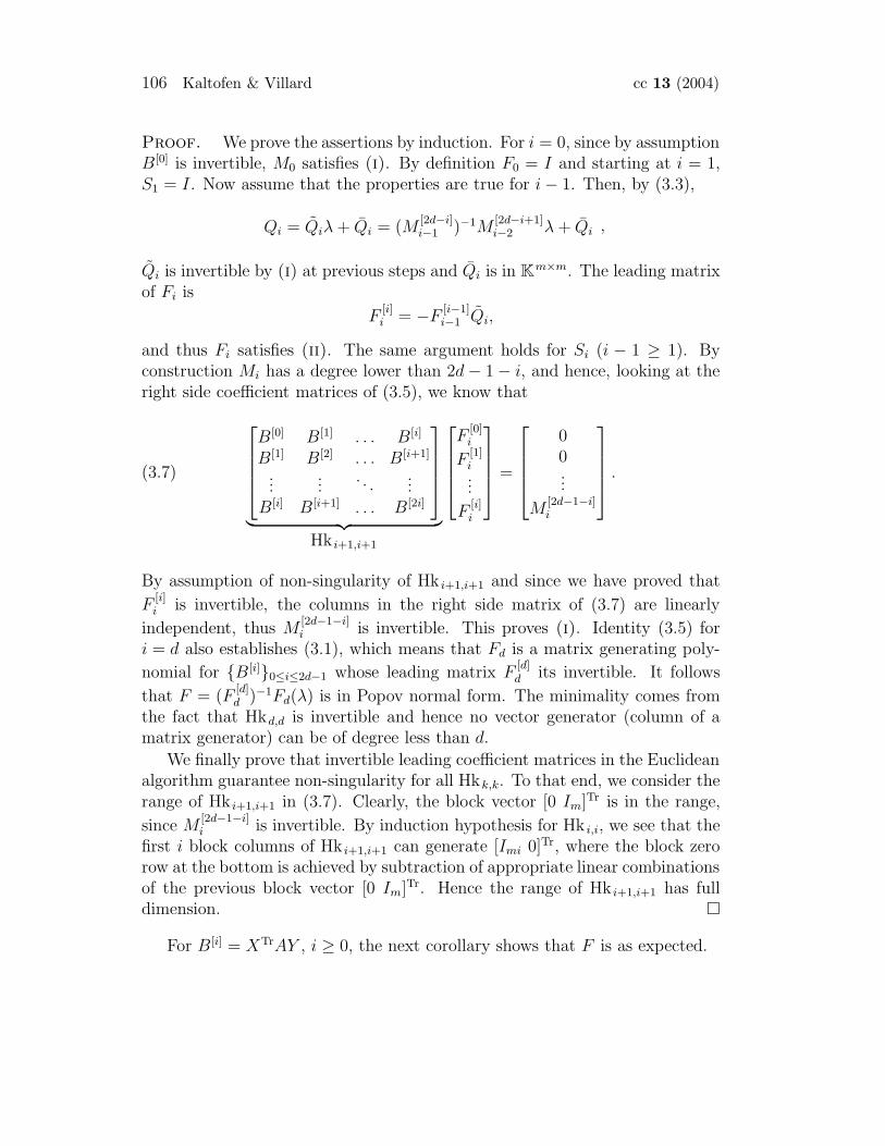
Proof. We prove the assertions by induction. For i = 0, since by assumptionB[0] is invertible, M0 satisfies (i). By definition F0 = I and starting at i = 1,S1 = I. Now assume that the properties are true for i− 1. Then, by (3.3),

Qi = Qiλ+ Qi = (M[2d−i]i−1 )−1M

[2d−i+1]i−2 λ+ Qi ,

Qi is invertible by (i) at previous steps and Qi is in Km×m. The leading matrixof Fi is

F[i]i = −F [i−1]

i−1 Qi,

and thus Fi satisfies (ii). The same argument holds for Si (i − 1 ≥ 1). Byconstruction Mi has a degree lower than 2d− 1− i, and hence, looking at theright side coefficient matrices of (3.5), we know that

(3.7)

B[0] B[1] . . . B[i]

B[1] B[2] . . . B[i+1]

......

. . ....

B[i] B[i+1] . . . B[2i]

︸︷︷︸Hk i+1,i+1

F[0]i

F[1]i...

F[i]i

=

00...

M[2d−1−i]i

.

By assumption of non-singularity of Hk i+1,i+1 and since we have proved that

F[i]i is invertible, the columns in the right side matrix of (3.7) are linearly

independent, thus M[2d−1−i]i is invertible. This proves (i). Identity (3.5) for

i = d also establishes (3.1), which means that Fd is a matrix generating poly-

nomial for {B[i]}0≤i≤2d−1 whose leading matrix F[d]d its invertible. It follows

that F = (F[d]d )−1Fd(λ) is in Popov normal form. The minimality comes from

the fact that Hkd,d is invertible and hence no vector generator (column of amatrix generator) can be of degree less than d.

We finally prove that invertible leading coefficient matrices in the Euclideanalgorithm guarantee non-singularity for all Hkk,k. To that end, we consider therange of Hk i+1,i+1 in (3.7). Clearly, the block vector [0 Im]Tr is in the range,

since M[2d−1−i]i is invertible. By induction hypothesis for Hk i,i, we see that the

first i block columns of Hk i+1,i+1 can generate [Imi 0]Tr, where the block zerorow at the bottom is achieved by subtraction of appropriate linear combinationsof the previous block vector [0 Im]Tr. Hence the range of Hk i+1,i+1 has fulldimension. �

For B[i] = XTrAY , i ≥ 0, the next corollary shows that F is as expected.


Corollary 3.8. Let A be in Kn×n, let B[i] = XTrAiY ∈ Km×m, i ≥ 0, andlet ν = md be the determinantal degree degλ(detFA,Y

X ). If the block Hankelmatrix Hkd,d(A,X, Y ) satisfies the assumption of Theorem 3.6 then F = FA,Y

X .

Proof. We know from (2.6) that ν is the maximum possible rank for theblock Hankel matrices associated to the sequence, thus the infinite one Hk∞,d+1

satisfies

rank Hk∞,d+1 = rank

B[0] B[1] . . . B[d]

B[1] B[2] . . . B[d+1]

......

...

= rank Hkd,d+1 = ν.

It follows that Hk∞,d+1 and Hkd,d+1 have the same nullspace, and F , which byTheorem 3.6 is a matrix generator for the truncated sequence {B [i]}0≤i≤2d−1, isa generator for the whole sequence. The argument used for the minimality ofF remains valid, hence F = FA,Y

X . �

Remark 3.9. In Theorem 3.6 and Corollary 3.8 we have only addressed thecase where the target determinantal degree is an exact multiple md of theblocking factor m. This can be assumed with no loss of generality for the algo-rithms in Sections 4 and 5 and the corresponding asymptotic costs in Section 6.Indeed, we will work there with ν = n and the input matrix A may be paddedto diag(A, I).

In the general case or in practice to avoid padding, the Euclidean algorithmleads to rankM

[d]d−1 = ν mod m ≤ m and requires a special last division step.

The minimum generator F = FA,YX has degree d = dν/me, with column degrees

[δ1, . . . , δm] = [d − 1, . . . , d− 1, d, . . . , d], where d− 1 is repeated mdν/me − νtimes (Villard 1997b, Proposition 6.1).

The above method can be combined with the recursive Knuth (1970)/Schon-hage (1971)/Moenck (1973) algorithm. If ω is the exponent of matrix multipli-cation then, as soon as the block Hankel matrix has the required rank profile,FA,YX may be computed with (nωd)1+o(1) operations in K. The required FFT-

based multiplication algorithms for matrix polynomials are described by Cantorand Kaltofen (1991).

3.2. Normal matrix remainder sequences over the integers. The nor-mality of the remainder sequence associated to a given matrix A essentiallycomes from the genericity of the projections. This may be partly seen in thescalar case for Lanczos algorithm from (Eberly & Kaltofen 1997, Lemma 4.1),


(Eberly 2002) or (Kaltofen & Lee 2003; Kaltofen et al. 2000) and in the blockcase from (Kaltofen 1995, Proposition 3) or (Villard 1997b, Proposition 6.1).

We show here that the block Hankel matrix has generic rank profile forgeneric projections, and then the integer case follows by randomization. Welet X and Y be two n×m matrices with indeterminate entries ξi,j and υi,j for1 ≤ i ≤ n and 1 ≤ j ≤ m. Let also ν be the maximum determinantal degreedefined by (2.13) in Theorem 2.12.

Lemma 3.10. With d = dν/me, the block Hankel matrix Hk d,d(A,X ,Y) hasrank ν and its principal minors of order i are non-zero for 1 ≤ i ≤ ν.

Proof. To simplify the presentation we only detail the case where ν is amultiple of m (see Remark 3.9). Let Kr i(A,Z) ∈ Kn×i be the block Krylovmatrix formed by the i first columns of [Z AZ . . . Ad−1Z] for 1 ≤ i ≤ ν. Thespecialization Z ∈ Kn×m of Y given in (Villard 1997b, Proposition 6.1) satisfies

(3.11) rank Kr i(A,Z) = i, 1 ≤ i ≤ ν.

We now argue, by specializing X and Y, that the target principal minors arenon-zero. If i ≤ m, using (3.11) one can find X ∈ Kn×i such that the rankof XTrKr i(A,Z) equals i. If m < i ≤ ν then one can find X ∈ Kn×m suchthat XTrKr i(A,Z) = [0 Jm], where Jm is the m ×m reversion matrix. HenceHkd,d(A,X, Z) has ones on its i-th anti-diagonal and zeros above, and thecorresponding principal minor of order i is (−1)bi/2c. �

The polynomial∏d

k=1 det Hkk,k(A,X ,Y) is non-zero of degree no more thanmd(d+ 1) in K[. . . , ξi,j, . . . , υi,j, . . .]. If the entries of X and Y are chosen uni-formly and independently from a finite set S ⊂ Z then, by the Schwartz/Zippellemma and Theorem 3.6, the associated matrix remainder sequence is normalwith probability at least 1−md(d+ 1)/|S|.

4. The block baby steps/giant stepsdeterminant algorithm

We shall present our algorithm for integer matrices. Generalizations to otherdomains, such as polynomial rings, are certainly possible. The algorithm fol-lows the Wiedemann paradigm (Wiedemann 1986, Chapter V) and uses ababy steps/giant steps approach for computing the sequence elements (Kaltofen1992). In addition, the algorithm blocks the projections (Coppersmith 1994).A key ingredient is that from the theory of realizations described in Section 2,it is possible to recover the characteristic polynomial of a preconditioning ofthe input matrix.


Algorithm Block Baby Steps/Giant Steps Determinant.Input: a matrix A ∈ Zn×n.Output: an integer that is the determinant of A, or “failure;” the algorithmfails with probability no more than 1/2.

Step 0. Let h = log2 Hd(A), where Hd(A) is a bound on the magnitude of thedeterminant of A, for instance, Hadamard’s bound (see, for example, vonzur Gathen & Gerhard 1999). To guarantee the probability of a successfulcompletion, the algorithm uses positive constants γ1, γ

′1 ≥ 1.

Choose a random prime integer p0 ≤ γ′1hγ1 and compute detA mod p0 by

LU-decomposition over Zp0 .If the result is zero, A is most likely singular, and the algorithm calls analgorithm for computing x ∈ Zn \ {0} with Ax = 0; see Remark 4.7 onpage 115 below. Note that the following steps would fail, for example, tocertify the determinant of the zero matrix.

Step 1. Precondition A in such a way that with high probability det(λI−A) =s1(λ) · · · smin{m,φ}, where s1, . . . , sφ are the invariant factors of λI−A andwhere m is the blocking factor that will be chosen in Step 2. We havetwo very efficient preconditioners at our disposal. The first is A ← DA,where D is a random diagonal matrix with the diagonal entries chosenuniformly and independently from a set S of integers (Chen et al. 2002,Theorem 4.3). The second by Turner (2001) is A← EA, where

E =

1 w1 0 . . . 0

0. . .

. . ....

.... . . 1 wn−1

0 . . . 0 1

, wi ∈ S.

The product DA is slightly cheaper than EA, but recovery of detA re-quires division by detD. Thus, all moduli that divide detD would haveto be discarded from the Chinese remainder algorithm below for the firstpreconditioner. Both preconditioners achieve s1(λ) = det(λI − A) withprobability 1− O(n2/|S|). Note that A is non-singular. We shall chooseS = {i | −bγ′2nγ2c ≤ i ≤ dγ′2nγ2e}, where γ2 ≥ 2 and γ′2 ≥ 1 are realconstants.

Step 2. Let the blocking factors be l = m = dnσ e, where σ = 1/3.Select random X, Y ∈ Sn×m.We will compute the sequence B [i] = XTrAiY for all 0 ≤ i < d2n/me =O(n1−σ) by utilizing our baby steps/giant steps technique (Kaltofen 1992).


Let the number of giant steps be s = dnτ e, where τ = 1/3, and let thenumber of baby steps be r = d2dn/me/se = O(n1−σ−τ ).

Substep 2.1. For j = 0, 1, . . . , r − 1 Do V [j] ← AjY ;

Substep 2.2. Z ← Ar;

Substep 2.3. For k = 1, 2, . . . , s− 1 Do (U [k])Tr ← XTrZk;

Substep 2.4. For j = 0, 1, . . . , r − 1 DoFor k = 0, 1, . . . , s− 1 Do B [kr+j] ← (U [k])TrV [j].

Step 3. Compute the minimum matrix generator FA,YX (λ) from the initial

sequence segment {B[i]}0≤i<2dn/me. Here we can use the method fromSection 3, padding the matrix so that m divides n (see Remark 3.9 on

page 107), and return “failure” whenever the coefficient F[i]i of the matrix

remainder polynomial is singular. For alternative methods, we refer toRemark 4.1 below the algorithm.

Step 4. If deg(detFA,YX ) < n return “failure” (this check may be redun-

dant, depending on which method was used in Step 3). Otherwise, sinceFA,YX (λ) is in Popov form we know that its determinant is monic and by

Theorem 2.12 we have detFA,YX (λ) = det(λI−A). Return detA = ∆(0),

or a value adjusted according to the preconditioner used in Step 1. �

Remark 4.1. As we have seen in Section 2.1 there are several alternatives forcarrying out Step 3 (Beckermann & Labahn 1994; Coppersmith 1994; Dickin-son et al. 1974; Forney, Jr. 1975; Giorgi et al. 2003; Kaltofen 1995; Rissanen1972; Thome 2002; Van Barel & Bultheel 1992). In Step 4 we require thatdetFA,Y

X (λ) = det(λI − A). In order to achieve the wanted bit complexity,we must stop any of the algorithms after having processed the first 2dn/meelements of (2.1). The algorithm used must then return a candidate matrix

polynomial F . Clearly, if Step 4 exposes deg(det F ) < n one knows that the

randomizations were unlucky. However, if deg(det F ) = n there still may be the

possibility that F 6= FA,YX due to a situation where the first 2dn/me elements

do not determine the generator, as would be the case in the two examplesgiven in Section 2. In order to achieve the Las Vegas model of randomizedalgorithmic complexity, verification of the computed generator is thus neces-sary here. For example, the algorithm used could do so by establishing thatrank Hkdn/me,dn/me(A,X, Y ) = n. Our algorithm from Section 3 implicitly does


so via Theorem 3.6 on page 105. One could do so explicitly by computing therank of Hk dn/me,dn/me modulo a random prime number.

We remark that the arithmetic cost of verifying that the candidate for F A,YX

is a generator for the block Krylov sequence {AiY }i≥0 is the same as Step 2.The reduction is seen by applying the transposition principle (Kaltofen 2000,Section 6): note that computing all B [i] is the block diagonal left product

[(XTr)1,∗ | (XTr)2,∗ | . . .

]·

. . . AiY . . . 0 0 · · · 00 . . . AiY . . . 0 · · · 0...

. . ....

0 0 · · · . . . AiY . . .

,

where (XTr)i,∗ denotes the i-th row of XTr. Computing∑

iAiY c[i], where

c[i] ∈ Km×m are the coefficients of FA,YX , is the block diagonal right product

. . . AiY . . . 0 0 · · · 00 . . . AiY . . . 0 · · · 0...

. . ....

0 0 · · · . . . AiY . . .

·

(c[0])∗,1(c[1])∗,1

...(c[0])∗,2(c[1])∗,2

...

,

where (c[i])∗,j denotes the j-th column of the matrix c[i]. One may also developan explicit baby steps/giant steps algorithm for computing

∑iA

iY c[i]. How-ever, because the integer lengths of the entries in c[i] are much larger than thoseof X and Y , we do not know how to keep the bit complexity low enough toallow verification of the candidate generator via verification as a block Krylovspace generator.

We shall first give the bit complexity analysis for our block algorithm underthe assumption that no subcubic matrix multiplication a la Strassen or sub-quadratic block Toeplitz solver/greatest common divisor algorithm a la Knuth/Schonhage is employed. We will investigate those best theoretically possiblerunning times in Section 6.

Theorem 4.2. Our algorithm computes the determinant of any non-singularmatrix A ∈ Zn×n with (n3+1/3 log ‖A‖)1+o(1) bit operations. Our algorithm uti-lizes (n1+1/3 + n log ‖A‖)1+o(1) random bits and either returns the correct de-terminant or returns “failure,” the latter with probability of no more than 1/2.


In our analysis, we will use modular arithmetic. The following lemma willbe used to establish the probability of getting a good reduction with primemoduli.

Lemma 4.3. Let γ ≥ 1 and γ ′ ≥ 1 be real constants. Then for all integersH ∈ Z≥2 that with h = 2 logeH ≤ 1.89 log2 H satisfy 10 ≤ h, h 6∈ [113, 113.6]and γ′ ≤ hγ, we have the probability estimate

(4.4) Prob(p divides H | p a prime integer, 2 ≤ p ≤ γ ′hγ) ≤ 25

8

γ

γ′hγ−1.

Proof. We have the following estimates for the distribution of prime num-bers: ∏

p primep≤x

p > eC1x, π(x) =∑

p primep≤x

1 >C2x

loge x, π(x) <

C3x

loge x,

where C1, C2 and C3 are positive constants. Explicit values for C1, C2 and C3

have been derived. We may choose C1 = 0.5 for x ≥ 10 (Rosser & Schoenfeld1962, Theorem 10 + explicit estimation for 10 ≤ x < 101), C2 = 0.8 for x ≥ 5(Rosser & Schoenfeld 1962, Corollary 1 to Theorem 2 and explicit estimationfor 10 ≤ x < 17), and C3 = 1.25 for x < 113 and x ≥ 113.6 (Rosser &Schoenfeld 1962, Corollary 2 to Theorem 2).

Since we have∏

p≤h p > eC1h = H, there are at most π(h) < C3h/loge hdistinct prime factors in H. The number of primes ≤ γ ′hγ is more thanC2γ

′hγ/(γ loge h + loge γ′), because from our assumptions we have γ ′hγ ≥ 10.

Therefore the probability for a random p to divide H is no more than, usingloge γ

′ ≤ γ loge h,

C3h/loge h

C2γ′hγ/(γ loge h+ loge γ′)≤ C3h/loge h

C2γ′hγ/(2γ loge h)≤ 2C3

C2

γ

γ′hγ−1. �

In the above Lemma 4.3 we have introduced the constant γ ′ so that it ispossible to choose γ = 1 and have a positive probability of avoiding a primedivisor of H.

Proof of Theorem 4.2. The unblocked version of the algorithm is fullyanalyzed by Kaltofen (2002) with the additional modification of early termi-nation when the determinant is small. That analysis uses a residue numbersystem (Chinese remaindering) for representing long integers, which we adoptfor the blocked algorithm. This adds the bit cost of generating a stream ofsufficiently large random primes (including p0 in Step 0).


Step 0 has by h = O(n log(n‖A‖)), which follows from Hadamard’s bound,the bit complexity (n3 + n2 log ‖A‖)1+o(1), the latter term constituting takingevery entry of A modulo p0. The failure probability of Step 0, that is whendetA ≡ 0 (mod p0) for non-singular A, is bounded by Lemma 4.3. Thus,for H = detA and appropriate choice of γ1 and γ′1 in Step 0 all non-singularmatrices will pass with probability no less than 9/10.

Step 1 increases log ‖DA‖ or log ‖EA‖ to no more than O((logn)2 log ‖A‖)and has bit cost (n3 log ‖A‖)1+o(1).

Steps 3 and 4 are performed modulo sufficiently many primes pl so thatdetA can be recovered via Chinese remaindering. Using pl ≥ 2, we obtain thevery loose count

(4.5) 1 ≤ l ≤ 2 log2(Hd A) = 2h = O(n log(n‖A‖)),the factor 2 accounting for recovery of negative determinants. Modular arith-metic becomes necessary to avoid length growth in the scalars in F A,Y

X duringSteps 3 and 4. We shall first estimate the probability of success, and then thebit complexity. The probabilistic analysis will also determine the size of theprime moduli.

The algorithm fails if:

(i) The preconditioners D or E in Step 1 do not yield det(λI−A) = s1(λ) · · ·smin{m,φ}, that with probability ≤ O(1/nγ2−2). As for Step 0, we select theconstant γ2, γ

′2 so that the preconditioners fail with probability ≤ 1/10.

(ii) The projectionsX, Y in Step 2 do not yield rank Hk dn/me,dn/me(A,X, Y )=n.Since for X = X and Y = Y with variables ξi,j, υi,j as entries full rank isachieved (see Section 2), we can consider an n×n non-singular submatrixΓ(X ,Y) of Hk dn/me,dn/me(A,X ,Y). By (DeMillo & Lipton 1978; Schwartz1980; Zippel 1979) we get

Prob(det Γ(X, Y ) = 0 | X, Y ∈ Sn×m) ≤ deg(det Γ)

|S| ≤ 2n

|S| ≤1

γ′2nγ2−1

.

If we use the matrix polynomial remainder sequence algorithm of Section 3for Step 3, we also fail if

∏1≤k<dn/me det Hkk,k(A,X, Y ) = 0, that with

probability no more than n(n/m + 1)/|S| ≤ (n1−σ + 1)/(2γ′2nγ2−1).

Again, the constants γ2, γ′2 are chosen so that the probability is ≤ 1/10.

(iii) The computation modulo one of the moduli pl fails for Step 3 or 4.Then pl divides det Γ(A,X, Y ). Since log |det(Γ(A,X, Y ))| = ((n2/m)×log ‖A‖)1+o(1), we may select the random moduli in the range

(4.6) 2 ≤ pl ≤ γ′3(n2−σ log ‖A‖)(1+o(1))γ3 = q.


where σ = 1/3 and γ3 ≥ 2, γ′3 ≥ 1 are constants. Note that in(4.6) the exponent 1 + o(1) captures derivable polylogarithmic factorsC1(logn)C2(log ‖A‖)C3 , where C1, C2, C3 are explicit constants. ByLemma 4.3 the probability that any one of the ≤ 2h moduli fails, i.e. di-vides det Γ(A,X, Y ), is no more than 2h/(n2−σ log ‖A‖)(1+o(1))(γ3−1). Bythe Hadamard estimate (4.5) we can make this probability no larger than1/10 via selecting the constants γ3, γ

′3 sufficiently large.

If we must also avoid divisors of∏

1≤k<dn/me det Hkk,k(A,X, Y ) for the ma-

trix polynomial remainder sequence algorithm, the range (4.6) increasesto pl ≤ γ′3(n3−2σ log ‖A‖)(1+o(1))γ3 .

(iv) The algorithms fails to compute sufficiently many random prime modulipl ≤ q (see (4.6)). There is now a deterministic algorithm of bit complexity(log pl)

12+o(1) for primality testing (Agrawal et al. 2002), which is notrequired but simplifies the theoretical analysis here. We pick k = 4h log qpositive integers ≤ q. The probability for each to be prime is ≥ 1/log q =ψ (provided q ≥ 17; Rosser & Schoenfeld 1962). By Chernoff boundsfor the tail of the binomial distribution, the probability that fewer than2h = (1− 1/2)ψk are prime is ≤ e−(1/2)2ψk/2 = 1/eh/2. Thus for h ≥ 5 theprobability of failing to find 2h primes is ≤ 1/10.

Cases (i)–(iv) together with Step 0 add up to a failure probability of ≤ 1/2.We conclude by estimating the number of bit operations for Steps 2–4.

Step 2 computes B[i] mod pl for 0 ≤ i < 2dn/me and 1 ≤ l ≤ 2h asfollows. First, all B[i] are computed as exact integers. For Substeps 2.1and 2.2, that requires O(n3 log r) arithmetic operations on integers of length(r log ‖A‖)1+o(1), in total (n4−σ−τ log ‖A‖)1+o(1) bit operations (recall that σ =τ = 1/3). Substeps 2.3 and 2.4 require O(smn2) arithmetic operations onintegers of length (rs log ‖A‖)1+o(1), again (n3+τ log ‖A‖)1+o(1) bit operations.Then all O((n/m)m2) entries of all B[i] are taken modulo pl with l in therange (4.5) and pl in (4.6). Straightforward remaindering would yield a total of(nmhrs log ‖A‖)1+o(1) bit operations, which is (n3(log ‖A‖)2)1+o(1). The com-plexity can be reduced to (n3 log ‖A‖)1+o(1) via a tree evaluation scheme (Ahoet al. 1974; Heindel & Horowitz 1971, Algorithm 8.4).2

Steps 3 and 4 are performed modulo all O(h) prime moduli pl. For eachprime the cost of extended Euclidean algorithm on matrix polynomials isO(m3(n/m)2) residue operations. Overall, the bit complexity of Steps 3 and 4

2Note that this speedup comes at a cost of an extra log-factor.


is again (n3+σ log ‖A‖)1+o(1). The number of required random bits in D or E,X and Y , and case (iv) above is immediate. �

It is possible to derive explicit values for the constants γ1, γ′1, γ2, γ′2, γ3, andγ′3 so that Theorem 4.2 holds. However, any implementation of the algorithmwould select reasonably small values. For example, all prime moduli would bechosen 32 or 64 bit in length. Since the method is Las Vegas, such choice onlyaffects the probability of not obtaining a result.

If Step 3 uses a Knuth/Schonhage half-GCD approach with FFT-basedpolynomial arithmetic for the Euclidean algorithm on matrix polynomials ofSection 3, the complexity for each modulus reduces to (m2n)1+o(1) residue op-erations. Thus, the overall complexity of Steps 3 and 4 reduces to (n2+2σ ×log ‖A‖)1+o(1) bit operations. For σ = 3/5 and τ = 1/5 the bit complexity ofthe algorithm is then (n3+1/5 log ‖A‖)1+o(1).

Remark 4.7. In order to state a Las Vegas bit complexity for the determinantof a general square matrix, we need to consider the cost of certifying singularityin Step 0 on page 109 above. In order to meet the complexity of Theorem 4.2on page 111 above we can use the algorithm by Dixon (1982). Reduction toa non-singular subproblem can be accomplished by methods of Kaltofen andSaunders (1991), and the rank is determined in a Monte Carlo manner via arandom prime modulus; see also (Villard 1988, p. 102).

5. Improved division-free complexity

Our baby steps/giant steps algorithm with blocking of Section 4 can be em-ployed to improve Kaltofen’s (1992) division-free complexity of the determinant(see also Seifullin 2003). Here we consider a matrix A ∈ Rn×n, where R is acommutative ring with a unit element. At task is to compute the determinantof A by ring additions, subtractions and multiplications. Blocking can improvethe number of ring operations from n3.5+o(1) (Kaltofen 1992) to n3+1/3+o(1),that without subcubic matrix multiplication or subquadratic Toeplitz/GCDalgorithms, and best possible from O(n3.0281) (Kaltofen 1992)3 to O(n2.6973).Our algorithm combines the blocked determinant algorithm with the elimina-tion of divisions technique of Kaltofen (1992). Our computational model iseither a straight-line program/arithmetic circuit or an algebraic random accessmachine (Kaltofen 1988). Further problems are to compute the characteristicpolynomial and the adjoint matrix of A.

3The proceedings paper gives an exponent 3.188; the smaller exponent is in a postnoteadded to the version posted on www.kaltofen.us/bibliography.


The main idea of Kaltofen (1992) follows Strassen (1973) and for the in-put matrix A computes the determinant of the polynomial matrix L(z) =C + z(A− C), where C ∈ Zn×n is a special integral matrix whose entries areindependent of the entries in A (see below). For ∆(z) = detL(z) we havedetA = ∆(1). All intermediate elements are represented as polynomials inR[z] or as truncated power series in R[[z]] and the “shift” matrix C determinesthem in such a manner that whenever a division by a polynomial or truncatedpower series is performed the constant coefficients are ±1. For the algorithmin Section 4 we not only pick a generalized shift matrix, now denoted by M ,but also concrete projection block vectors X ∈ Zn×m and Y ∈ Zn×m. No ran-domization is necessary, as M is a “good” input matrix (φ = m) and X and Y

are “good” projections, we have detFL(z),YX (λ) = det(λI − L(z)).

The matrices M , X and Y are block versions of the ones constructed byKaltofen (1992). Suppose that the blocking factor m is a divisor of n, the

dimension of A. This we can always arrange by padding A to

[A 00 I

]. Let

d = n/m and

ai =

(i

bi/2c

), ci = −(−1)b(d−i+1)/2c

(b(d+ i)/2ci

),

C =

0 1 0 . . . 0

0 0 1. . . 0

......

. . .. . . 0

0 0 0 1c0 c1 . . . cd−2 cd−1

, v =

a0

a1...

ad−1

.

We have shown (Kaltofen 1992) that for the sequence ai = eTr1 C

iv, whereeTr

1 =[1 0 . . . 0

]∈ Z1×d is the first d-dimensional unit (row) vector, the

Berlekamp/Massey algorithm divides by only ±1. We now define

M =

C 0 . . . 0

0 C. . . 0

... 0. . .

...0 . . . 0 C

∈ Z

n×n,

X =

e1 0 . . . 0

0 e1. . . 0

... 0. . .

...0 . . . e1

∈ Z

n×m, Y =

v 0 . . . 0

0 v. . . 0

... 0. . .

...0 . . . v

∈ Z

n×m.


By construction, the algorithm for computing the determinant of Section 4 per-formed now with the matrices X,M, Y results in a minimum matrix generator

FM,YX (λ) = (λd − cd−1λ

d−1 − · · · − c0)Im,

where Im is the m × m identity matrix. Furthermore, this generator can becomputed from the sequence of block vectors B [i] = aiIm by a matrix Euclideanalgorithm (see Section 3) in which all leading coefficient matrices are equalto ±Im.

The arithmetic cost for executing the block baby steps/giant steps algorithmon the polynomial matrix L(z) = M+z(A−M) is related to the bit complexityof Section 4. Now the intermediate lengths are the degrees in z of the com-puted polynomials in R[z]. Therefore, the matrices XTrL(z)iY ∈ R[z]m×m canbe computed for all 0 ≤ i < 2d in n3+1/3+o(1) ring operations. In the matrixEuclidean algorithm for Step 3 we perform truncated power series arithmeticmodulo zn+1. The arithmetic cost is (d2m3n)1+o(1) ring operations for the clas-sical Euclidean algorithm with FFT-based power series arithmetic. For the lat-ter, we employ a division-free FFT-based polynomial multiplication algorithm(Cantor & Kaltofen 1991). Finally, to obtain the characteristic polynomial,we may slightly extend Step 4 on page 110 and compute the entire deter-

minant of FL(z),YX (λ) division-free in truncated power series arithmetic over

R[z, λ] mod (zn+1, λn+1) (a different approach is given at the end of Section 6).For this last step we can use our original division-free algorithm (Kaltofen 1992)and achieve arithmetic complexity (m3.5n2)1+o(1). We have proven the followingtheorem.

Theorem 5.1. Our algorithm computes the characteristic polynomial of anymatrix A ∈ Rn×n with (n3+1/3)1+o(1) ring operations in R. By the resultsof Baur and Strassen (1983) the same complexity is obtained for the adjointmatrix, which can be symbolically defined as det(A)A−1.

6. Using fast matrix multiplication

As stated in the Introduction, by use of subcubic matrix multiplication algo-rithms the worst case bit complexity of the block algorithms in Sections 4 and5 can be brought below cubic complexity in n. We note that taking the n2

entries of the input matrix modulo n prime residues is already a cubic processin n; our algorithms therefore proceed differently.

Now let ω by the exponent for fast matrix multiplication. By Coppersmithand Winograd (1990) we may set ω = 2.375477. The considerations in thissection are of a purely theoretical nature.


Substep 2.1 in Section 4 is done by repeated doubling as in[A2µY A2µ+1Y . . . A2µ+1−1Y

]= A2µ

[Y AY . . . A2µ−1

Y]

for µ = 0, 1, . . . .

Therefore the bit complexity for Substeps 2.1 and 2.2 is (nωr log ‖A‖)1+o(1) withan exponent ω + 1 − σ − τ for n. Note that σ and τ determine the blockingfactor and number of giant steps, and will be chosen later so as to minimizethe complexity.

Substep 2.3 both splits the integer entries in U [k] into chunks of length(r log ‖A‖)1+o(1), which is the bit length of the entries in Z. There are at mosts1+o(1) such chunks. Thus each block vector times the matrix product (U [k])TrZis a rectangular matrix product of dimensions (ms)1+o(1)×n by n×n. We nowappeal to fast methods for rectangular matrices (Coppersmith 1997) (we seemnot to need the results of Huang & Pan 1998), which show how to multiply ann× n matrix by an n× ν matrix in nω−θ+o(1)νθ+o(1) arithmetic operations (byblocking the n × n matrix into (t × t)-sized blocks and the n × ν matrix into(t×tζ)-sized blocks such that n/t = ν/tζ and that the individual block productsonly take t2+o(1) arithmetic steps each), where θ = (ω − 2)/(1− ζ) with ζ =0.2946289. There are s such products on integers of length (r log ‖A‖)1+o(1),so the bit complexity for Substep 2.3 is (snω−θ(ms)θr log ‖A‖)1+o(1) with anexponent ω + 1− σ + (σ + τ − 1)θ for n.

Step 3 for each individual modulus can be performed by the method pre-sented in Section 3 in (mωn/m)1+o(1) residue operations. For all ≤ 2h moduliwe get a total bit complexity for Step 3 of (mω−1n2 log ‖A‖)1+o(1) with an ex-ponent 2 + σ(ω − 1) for n.

The bit complexities of Substep 2.4 and Step 4 are dominated by the com-plexities of other steps.

All of the above bit costs lead to total bit complexity of (nη log ‖A‖)1+o(1),where the exponent η depends on the use matrix multiplication exponents ωand ζ. Table 6.1 displays the optimal values of η for selected exponents togetherwith the exponents for the blocking factor and giant stepping that attain theoptimum. Line 1 is the symbolic solution, Line 2 gives the best exponentthat we have achieved. Line 3 is the solution without appealing to fasterrectangular matrix multiplication schemes. Line 4 corresponds to the commentsbefore Remark 4.7 on page 115, and line 5 uses Strassen’s original subquadraticmatrix multiplication algorithm. Line 6 exhibits the slowdown without fasterrectangular matrix multiplication algorithms. Line 7 is our complexity for ahypothetical quadratic matrix multiplication algorithm.

An issue arises whether the singularity certification in Step 0 of our algo-rithm can be accomplished at a matching or lower bit complexity than the ones


ω ζ η σ τ

1 ω ζ ω + 1−ζω2−(2+ζ)ω+2

1− ω−(1+ζ)ω2−(2+ζ)ω+2

ω−2ω2−(2+ζ)ω+2

2 2.375477 0.2946289 2.697263 0.506924 0.171290

3 ω 0 ω + 1(ω−1)2+1

1− ω−1(ω−1)2+1

ω−2(ω−1)2+1

4 3 0 3 + 15

35

15

5 log2(7) 0 3.041738 0.576388 0.189230

6 2.375477 0 2.721267 0.524375 0.129836

7 2 0 2 + 12

12

0

Table 6.1: Determinantal bit/division-free complexity exponent η.

given above for the determinant. We refer to possible approaches by Muldersand Storjohann (2004) and Storjohann (2004).

The above analysis applies to our algorithm in Section 5 and yields forthe determinant and adjoint matrix a division-free complexity of O(n2.697263)ring operations. To our knowledge, this is the best known to date. For thedivision-free computation of the characteristic polynomial the homotopy is al-tered, because the computation of detF

L(z),YX (λ) mod (zn+1, λn+1) in Step 4 (see

Section 5) seems to require too many ring operations. One instead computes

det(M − zAM) = det(I − zA) detM = ±zn det((1/z)I − A)

by replacing A − M by AM in the original determinant algorithm. SincedetM = ±1 one thus gets (the reverse of) the characteristic polynomial inO(n2.697263) ring operations as well.

A Maple 7 worksheet that contains our exponent calculations is posted athttp://www.kaltofen.us/bibliography.

7. Integer characteristic polynomial and normal forms

As already seen in Sections 5 and 6 over an abstract ring R, our determinantalgorithm also computes the adjoint matrix and the characteristic polynomial.In the case of integer matrices, although differently from the algebraic setting,the algorithm of Section 4 may also be extended to solving other problems.We briefly mention two extensions. For A ∈ Zn×n we shall first see that thealgorithm leads to the characteristic polynomial of a preconditioning of A andconsequently to the Smith normal form of A. We shall then see how F A,Y

X may


be used to compute the Frobenius normal form of A and hence its characteristicpolynomial. Note that the exponents in our bit complexity are of the same orderas those discussed for the determinant problem in Table 6.1.

7.1. Smith normal form of integer matrices. A randomized Monte Carloalgorithm for computing the Smith normal form S ∈ Zn×n of an integer matrixA ∈ Zn×n of rank r may be designed by combining the algorithm of Section 4with the approach of Giesbrecht (2001). Here we improve on the best previouslyknown randomized algorithm of Eberly et al. (2000). The current estimate fora deterministic computation of the form is (nω+1 log ‖A‖)1+o(1) (Storjohann1996).

The Smith normal form over Z is defined in a way similar to what we haveseen in Section 2.2 for polynomial matrices. The Smith form S is an equivalentdiagonal matrix in Zn×n, with diagonal elements s1, s2, . . . , sr, 0, . . . , 0 such thatsi divides si−1 for 2 ≤ i ≤ r. The si’s are the invariant factors of A (Newman1972).

Giesbrecht’s approach reduces the computation of S to the computation ofthe characteristic polynomials of the matrices D

(i)1 T (i)D

(i)2 A for l = (logn +

log log ‖A‖)1+o(1) random choices of diagonal matrices D(i)1 and D

(i)2 and of

Toeplitz matrices T (i), 1 ≤ i ≤ l. The invariant factors may be computedfrom the coefficients of these characteristic polynomials. The preconditioningB ← D

(i)1 T (i)D

(i)2 A ensures that the minimum polynomial fB of B is squarefree

(Giesbrecht 2001, Theorem 1.4) (see also Chen et al. 2002 for such precondi-tionings). Hence if fB denotes the largest divisor of fB such that fB(0) 6= 0,we have r = rankB = deg fB, which is −1 + deg fB if A is singular. ByTheorem 2.12, for random X and Y we shall have, with high probability,∆(λ) = detFB,Y

X (λ) = λk1fB(λ) = λk2 fB(λ) for two positive integers k1 andk2 that depend on the rank and on the blocking factor m. The needed charac-teristic polynomials λn−rfB and then the Smith form are thus obtained fromthe determinants of l matrix generating polynomials.

To ensure a high probability of success, the computations are done withD

(i)1 , D

(i)2 and T (i) chosen over a ring extension RZ of degree O((logn)2) of Z, in

combination with Chinese remaindering modulo (n log ‖A‖)1+o(1) primes (Gies-brecht 2001, Theorem 4.2). For one choice of B(i), the cost overhead comparedto Step 4 in Section 4 is the one of computing the entire determinant of the

m × m matrix polynomial FB(i),YX of degree d = dn/me. Over a field, by

(Storjohann 2002, Proposition 24) or (Storjohann 2003, Proposition 41) sucha determinant is computed in (mωd)1+o(1) arithmetic operations. Using the(n log ‖A‖)1+o(1) primes and the fact that the ring extension RZ has degree


O((logn)2), detFB(i),YX ∈ RZ[λ] is thus computed in (n2+σ(ω−1) log ‖A‖)1+o(1)

bit operations.From this we see that the cost of computing the l characteristic polynomials,

which is the dominant cost in computing the Smith form, corresponds to theestimate already taken into account for Step 3 of the determinant algorithm.Hence the values of η in Table 6.1 remain valid for the computation of theSmith normal form using a randomized Monte Carlo algorithm.

7.2. Integer characteristic polynomial and Frobenius normal form.As used above, a direct application of Section 4 leads to the characteristicpolynomial of a preconditioning of A. To compute the characteristic polyno-mial of A itself, we extend our approach using the Frobenius normal form andthe techniques of Storjohann (2000b). The Frobenius normal form of A ∈ Zn×nis a block diagonal matrix in Zn×n similar to A. Its diagonal blocks are the com-panion matrices for the invariant factors s1(λ), . . ., sφ(λ) of λI −A. Hence the

characteristic polynomial det(λI − A) =∏φ

i=1 si(λ) is directly obtained fromthe normal form. Our result is a randomized Monte Carlo algorithm which im-proves on previous complexity estimates for computing the characteristic poly-nomial or the Frobenius normal form over Z (Storjohann 2000a, Table 10.1).The certified randomized algorithm of Giesbrecht and Storjohann (2002) uses(nω+1 log ‖A‖)1+o(1) bit operations.

By Theorem 2.12 on page 102, if we avoid the preconditioning step (Step 1)in the determinant algorithm on page 109 in Section 4, the computation leadsto FA,Y

X (λ) and to

detFA,YX (λ) =

min{m,φ}∏

i=1

si(λ).

The first invariant factor s1(λ) is the minimum polynomial fA of A, hencedetFA,Y

X is a multiple of fA and a factor of the characteristic polynomial inZ[λ]. Following the cost analysis of the previous Section 7.1 for the determinantof the matrix generating polynomial, the exponents in Table 6.1 are thus validfor the computation of detFA,Y

X . The square free part fAsqfr of detFA,YX may be

deduced in (n2 log ‖A‖)1+o(1) bit operations (Gerhard 2001, Theorem 11).From the Frobenius normal form of A modulo a random prime p, fAsqfr allows

a multifactor Hensel lifting for reconstructing the form over Z (Storjohann2000b). With high probability, λI − A also has φ invariant factors modulo p.We denote them by s1, . . . , sφ. They can be decomposed into φ products

si = tei11 . . . teimm , 1 ≤ i ≤ φ,


for a GCD-free family {t1, . . . , tm} of square free polynomials in Fp[λ] and forindices (ei1, . . . , eim) ∈ Zm>0, 1 ≤ i ≤ φ. This decomposition is computed in(n2 log p)1+o(1) bit operations (Bach & Shallit 1996, Section 4.8). With highprobability we also have

t1t2 . . . tm = fAsqfr mod p.

The latter factorization can be lifted, for instance using the algorithm of (vonzur Gathen & Gerhard 1999, §15.5), into a family {t1, . . . , tm} of polynomialsmodulo a sufficiently high power k of p. With high probability, the invariantfactors of λI − A over Z and the Frobenius form of A may finally be obtainedas the following combinations of the ti’s:

si = tei11 . . . teimm mod pk, 1 ≤ i ≤ φ,

with coefficients reduced in the symmetric range.In addition to the computation of FA,Y

X (λ), the dominant cost is the cost ofthe lifting. Any divisor of the characteristic polynomial has a coefficient size of(n log ‖A‖)1+o(1) (for instance see Giesbrecht & Storjohann 2002, Lemma 2.1)hence one can take k = (n log ‖A‖)1+o(1). The polynomials t1, . . . , tm are thuscomputed in (n2 log ‖A‖)1+o(1) bit operations (von zur Gathen & Gerhard 1999,Theorem 15.18). We may conclude that the values of the exponent of η inTable 6.1 are valid for the randomized computation of the Frobenius normalform and the characteristic polynomial of an integer matrix.

Theorem 5.4 by Pan (2002) states a Las Vegas bit complexity of (n16/5×log ‖A‖)1+o(1) for the Frobenius factors of a matrix A ∈ Zn×n by a differentmethod. Victor Pan has told us on May 13, 2004 that his proof of his claimcurrently has a flaw.

8. Concluding remarks

Our baby steps/giant steps and blocking techniques apply to entry domainsother than the integers, like polynomial rings and algebraic number rings. Wewould like to add that if the entries are polynomials over a possibly finitefield, there are additional new techniques possible (Jeannerod & Villard 2004;Mulders & Storjohann 2003; Storjohann 2002, 2003). Storjohann (2004) hasextended his 2003 techniques to construct a Las Vegas algorithm that computesdetA where A ∈ Zn×n in (nω log ‖A‖)1+o(1) bit operations, when n×n matricesare multiplied in O(nω) algebraic operations. The best known division-freecomplexity of the determinant remains at O(n2.697263) as stated in Section 5 andSection 6. Furthermore, the best known bit-complexity of the characteristic


polynomial of an integer matrix is to our knowledge the one in Section 7.2,namely (n2.697263 log ‖A‖)1+o(1).

For the classical matrix multiplication exponent ω = 3, the bit complexityof integer matrix determinants is thus proportional to nη+o(1) as follows: η =3 + 1

2(Eberly et al. 2000; Kaltofen 1992, 2002), η = 3 + 1

3(Theorem 4.2 on

page 111), η = 3+ 15

(line 4 in Table 6.1 on page 119), η = 3 (Storjohann 2004).Together with the algorithms discussed in Section 1 on page 94 that performwell on propitious inputs, such a multitude of results poses a problem for thepractitioner: which of the methods can yield faster procedures in computeralgebra systems? With William J. Turner we have implemented our babysteps/giant steps algorithm (Kaltofen 1992, 2002) in Maple 6 with mixed resultsin comparison to Gaussian elimination and Chinese remaindering. The mainproblem seems the overhead hidden in the no(1)-factor. For example, for n1 =10000 one has (log2 n1)/n

1/31 > 0.616, which means that saving a factor of

n1/3 at the cost of a factor log2 n may for practical considerations be quiteimmaterial. In addition, one also needs to consider other properties, such asthe required intermediate space and whether the algorithm is easily parallelized.We believe that the latter may be the most important advantage in practice ofour block approach (cf. Coppersmith 1994; Kaltofen 1995).

The reduction of the bit complexity of an algebraic problem below that ofits known algebraic complexity times the bit length of the answer should raiseimportant considerations for the design of generic algorithms with abstractcoefficient domains (Jenks et al. 1988) and for the interpretation of algebraiclower bounds for low complexity problems (Strassen 1990). We demonstratethat the interplay between the algebraic structure of a given problem and thebits of the intermediately computed numbers can lead to a dramatic reductionin the bit complexity of a fundamental mathematical computation task.

Acknowledgements

We thank William J. Turner for his observations on the practicality of ourmethod, Mark Giesbrecht for reporting to us the value of the smallest exponentin (Eberly et al. 2000) prior to its publication, Elwyn Berlekamp for commentson the Berlekamp/Massey algorithm, and the three referees for their comments.

This material is based on work supported in part by the National ScienceFoundation (USA) under Grants Nos. DMS-9977392, CCR-9988177 and CCR-0113121 (Kaltofen) and by CNRS (France) Actions Incitatives No 5929 et SticLinBox 2001 (Villard).

An extended abstract of this paper is (Kaltofen & Villard 2001).


References

Note: many of the authors’ publications cited below are accessible throughlinks in their webpages listed under their addresses.

J. Abbott, M. Bronstein & T. Mulders (1999). Fast deterministic computationof determinants of dense matrices. In ISSAC 99, Proc. 1999 Internat. Symp. SymbolicAlgebraic Comput., S. Dooley (ed.), ACM Press, New York, 181–188.

M. Agrawal, N. Kayal & Nitin Saxena (2002). PRIMES is in P. Manuscript.Available from http://www.cse.iitk.ac.in/news/primality.pdf.

A. Aho, J. Hopcroft & J. Ullman (1974). The Design and Analysis of Algo-rithms. Addison and Wesley, Reading, MA.

E. Bach & J. Shallit (1996). Algorithmic Number Theory. Volume 1: EfficientAlgorithms. The MIT Press, Cambridge, MA.

W. Baur & V. Strassen (1983). The complexity of partial derivatives. Theoret.Comput. Sci. 22, 317–330.

B. Beckermann & G. Labahn (1994). A uniform approach for fast computationof matrix-type Pade approximants. SIAM J. Matrix Anal. Appl. 15, 804–823.

R. P. Brent, F. G. Gustavson & D. Y. Y. Yun (1980). Fast solution of Toeplitzsystems of equations and computation of Pade approximants. J. Algorithms 1, 259–295.

R. P. Brent, S. H. Gao & A. G. B. Lauder (2003). Random Krylov spaces overfinite fields. SIAM J. Discrete Math. 16, 276–287.

H. Bronnimann, I. Emiris, V. Pan & S. Pion (1999). Sign determination inresidue number systems. Theoret. Comput. Sci. 210, 173–197.

H. Bronnimann & M. Yvinec (2000). Efficient exact evaluation of signs of deter-minants. Algorithmica 27, 21–56.

W. S. Brown & J. F. Traub (1971). On Euclid’s algorithm and the theory ofsubresultants. J. ACM 18, 505–514.

D. G. Cantor & E. Kaltofen (1991). On fast multiplication of polynomials overarbitrary algebras. Acta Inform. 28, 693–701.

L. Chen, W. Eberly, E. Kaltofen, B. D. Saunders, W. J. Turner &G. Villard (2002). Efficient matrix preconditioners for black box linear algebra.Linear Algebra Appl. 343–344, 119–146.


K. L. Clarkson (1992). Safe and efficient determinant evaluation. In Proc. 33rdAnnual Sympos. Foundations of Comput. Sci., IEEE Comput. Soc. Press, Los Alami-tos, CA, 387–395.

D. Coppersmith (1994). Solving homogeneous linear equations over GF(2) viablock Wiedemann algorithm. Math. Comp. 62, 333–350.

D. Coppersmith (1997). Rectangular matrix multiplication revisited. J. Complexity13, 42–49.

D. Coppersmith & S. Winograd (1990). Matrix multiplication via arithmeticprogressions. J. Symbolic Comput. 9, 251–280.

R. A. DeMillo & R. J. Lipton (1978). A probabilistic remark on algebraicprogram testing. Inform. Process. Lett. 7, 193–195.

B. W. Dickinson, M. Morf & T. Kailath (1974). A minimal realization algo-rithm for matrix sequences. IEEE Trans. Automat. Control AC-19, 31–38.

J. Dixon (1982). Exact solution of linear equations using p-adic expansions. Numer.Math. 40, 137–141.

J. L. Dornstetter (1987). On the equivalence between Berlekamp’s and Euclid’salgorithms. IEEE Trans. Inform. Theory 33, 428–431.

W. Eberly (2002). Avoidance of look-ahead in Lanczos by random projections.Manuscript in preparation.

W. Eberly, M. Giesbrecht & G. Villard (2000). On computing the determinantand Smith form of an integer matrix. In Proc. 41st Annual Sympos. Foundations ofComput. Sci., IEEE Comput. Soc. Press, Los Alamitos, CA, 675–685.

W. Eberly & E. Kaltofen (1997). On randomized Lanczos algorithms. In Kuchlin(1997), 176–183.

I. Z. Emiris (1998). A complete implementation for computing general dimensionalconvex hulls. Int. J. Comput. Geom. Appl. 8, 223–254.

G. D. Forney, Jr. (1975). Minimal bases of rational vector spaces, with applica-tions to multivariable linear systems. SIAM J. Control 13, 493–520.

J. von zur Gathen & J. Gerhard (1999). Modern Computer Algebra. CambridgeUniv. Press, Cambridge.

J. Gerhard (2001). Fast modular algorithms for squarefree factorization and Her-mite integration. Appl. Algebra Engrg. Comm. Comput. 11, 203–226.


M. Giesbrecht (2001). Fast computation of the Smith form of a sparse integermatrix. Comput. Complexity 10, 41–69.

M. Giesbrecht & A. Storjohann (2002). Computing rational forms of integermatrices. J. Symbolic Comput. 34, 157–172.

P. Giorgi, C.-P. Jeannerod & G. Villard (2003). On the complexity of poly-nomial matrix computations. In Sendra (2003), 135–142.

L. E. Heindel & E. Horowitz (1971). On decreasing the computing time formodular arithmetic. In Conference Record, IEEE 12th Annual Sympos. on Switchingand Automata Theory, 126–128.

X. H. Huang & V. Y. Pan (1998). Fast rectangular matrix multiplication andapplications. J. Complexity 14, 257–299.

C.-P. Jeannerod & G. Villard (2004). Essentially optimal computation of theinverse of generic polynomial matrices. J. Complexity, to appear. Available fromhttp://perso.ens-lyon.fr/gilles.villard.

R. D. Jenks, R. S. Sutor & S. M. Watt (1988). Scratchpad II: An abstractdatatype system for mathematical computation. In Mathematical Aspects of Sci-entific Software, J. R. Rice (ed.), IMA Vol. Math. Appl. 14, Springer, New York,157–182.

T. Kailath (1980). Linear Systems. Prentice-Hall.

E. Kaltofen (1988). Greatest common divisors of polynomials given by straight-line programs. J. ACM 35, 231–264.

E. Kaltofen (1992). On computing determinants of matrices without divisions. InProc. 1992 Internat. Sympos. Symbolic Algebraic Comput. (ISSAC’92), P. S. Wang(ed.), ACM Press, New York, 342–349.

E. Kaltofen (1995). Analysis of Coppersmith’s block Wiedemann algorithm forthe parallel solution of sparse linear systems. Math. Comput. 64, 777–806.

E. Kaltofen (2000). Challenges of symbolic computation: my favorite open prob-lems. J. Symbolic Comput. 29, 891–919. With an additional open problem by R. M.Corless and D. J. Jeffrey.

E. Kaltofen (2002). An output-sensitive variant of the baby steps/giant stepsdeterminant algorithm. In Mora (2002), 138–144.

E. Kaltofen & W.-S. Lee (2003). Early termination in sparse interpolation algo-rithms. J. Symbolic Comput. 36, 365–400.


E. Kaltofen, W.-S. Lee & A. A. Lobo (2000). Early termination in Ben-Or/Tiwari sparse interpolation and a hybrid of Zippel’s algorithm. In Proc. 2000Internat. Sympos. Symbolic Algebraic Comput. (ISSAC’00), C. Traverso (ed.), ACMPress, New York, 192–201.

E. Kaltofen & J. May (2003). On approximate irreducibility of polynomials inseveral variables. In Sendra (2003), 161–168.

E. Kaltofen & B. D. Saunders (1991). On Wiedemann’s method of solvingsparse linear systems. In Proc. AAECC-9, H. F. Mattson et al. (eds.) Lecture Notesin Comput. Sci. 539, Springer, Heidelberg, 29–38.

E. Kaltofen & G. Villard (2001). On the complexity of computing determi-nants. In Proc. Fifth Asian Symposium on Computer Mathematics (ASCM 2001),K. Shirayanagi and K. Yokoyama (eds.), Lecture Notes Ser. Comput. 9, World Sci.,Singapore, 13–27.

E. Kaltofen & G. Villard (2004). Computing the sign or the value of thedeterminant of an integer matrix, a complexity survey. J. Comput. Appl. Math.162, 133–146.

D. E. Knuth (1970). The analysis of algorithms. In Congres Int. Math., Nice,Volume 3, 269–274.

W. Kuchlin (ed.) (1997). ISSAC 97, Proc. 1997 Internat. Sympos. Symbolic Alge-braic Comput. ACM Press, New York.

R. T. Moenck (1973). Fast computation of GCDs. In Proc. 5th ACM Sympos.Theory Comp., 142–151.

T. Mora (ed.) (2002). ISSAC 2002 Proc. 2002 Internat. Sympos. Symbolic AlgebraicComput. ACM Press, New York.

T. Mulders & A. Storjohann (2003). On lattice reduction for polynomial ma-trices. J. Symbolic Comput. 35, 377–401.

T. Mulders & A. Storjohann (2004). Certified dense linear system solving.J. Symbolic Comput. 37 (2004), 485–510.

M. Newman (1972). Integral Matrices. Academic Press.

V. Y. Pan (1988). Computing the determinant and the characteristic polynomial ofa matrix via solving linear systems of equations. Inform. Process. Lett. 28, 71–75.


V. Y. Pan (2002). Randomized acceleration of fundamental matrix computations.In Proc. STACS 2002, Lecture Notes in Comput. Sci. 2285, Springer, Heidelberg,215–226.

M. S. Paterson & L. J. Stockmeyer (1973). On the number of nonscalar mul-tiplications necessary to evaluate polynomials. SIAM J. Comput. 2, 60–66.

V. M. Popov (1970). Some properties of control systems with irreducible matrix-transfer functions. In Seminar on Differential Equations and Dynamical Systems, II(College Park, MD, 1969), Lecture Notes in Math. 144, Springer, Berlin, 169–180.

J. Rissanen (1972). Realizations of matrix sequences. Technical Report RJ-1032,IBM Research, Yorktown Heights, NY.

J. B. Rosser & L. Schoenfeld (1962). Approximate formulas of some functionsof prime numbers. Illinois J. Math. 6, 64–94.

A. Schonhage (1971). Schnelle Berechnung von Kettenbruchentwicklungen. ActaInform. 1, 139–144.

J. T. Schwartz (1980). Fast probabilistic algorithms for verification of polynomialidentities. J. ACM 27, 701–717.

T. R. Seifullin (2003). Acceleration of computation of determinants and charac-teristic polynomials without divisions. Cybernet. Systems Anal. 39, 805–815.

J. R. Sendra (ed.) (2003). ISSAC 2003, Proc. 2003 Internat. Sympos. SymbolicAlgebraic Comput. ACM Press, New York.

A. Storjohann (1996). Near optimal algorithms for computing Smith normal formsof integer matrices. In ISSAC 96, Proc. 1996 Internat. Sympos. Symbolic AlgebraicComput., Y. N. Lakshman (ed.), ACM Press, New York, 267–274.

A. Storjohann (2000a). Algorithms for matrix canonical forms. Dissertation, SwissFederal Institute of Technology (ETH), Zurich.

A. Storjohann (2000b). Computing the Frobenius form of a sparse integer matrix.Paper to be submitted.

A. Storjohann (2002). Higher-order lifting. In Mora (2002), 246–254.

A. Storjohann (2003). High-order lifting and integrality certification. J. SymbolicComput. 36, 613–648.


A. Storjohann (2004). The shifted number system for fast linear algebra on integermatrices. Technical Report CS-2004-18, School of Computer Science, University ofWaterloo, http://www.scg.uwaterloo.ca/~astorjoh/publications.html.

V. Strassen (1973). Vermeidung von Divisionen. J. Reine Angew. Math. 264,182–202.

V. Strassen (1990). Algebraic complexity theory. In Handbook of TheoreticalComputer Science, Algorithms and Complexity, J. van Leeuwen (ed.), Volume A,Elsevier, Amsterdam, 633–672.

Y. Sugiyama, M. Kasahara, S. Hirasawa & T. Namekawa (1975). A methodfor solving key equation for decoding Goppa codes. Inform. and Control 27, 87–99.

E. Thome (2002). Subquadratic computation of vector generating polynomials andimprovements of the block Wiedemann method. J. Symbolic Comput. 33, 757–775.

W. J. Turner (2001). A note on determinantal divisors and matrix preconditioners.Paper to be submitted.

W. J. Turner (2002). Black box linear algebra with the LINBOX library. Ph.D.thesis, North Carolina State Univ., Raleigh, NC, 193 pp.

M. Van Barel & A. Bultheel (1992). A general module theoretic framework forvector M-Pade and matrix rational interpolation. Numerical Algorithms 3, 451–462.

G. Villard (1988). Calcul Formel et Parallelisme : Resolution de SystemesLineaires. Ph.D. thesis, Institut National Polytechnique de Grenoble.

G. Villard (1997a). Further analysis of Coppersmith’s block Wiedemann algorithmfor the solution of sparse linear systems. In Kuchlin (1997), 32–39.

G. Villard (1997b). A study of Coppersmith’s block Wiedemann algorithm usingmatrix polynomials. Rapport de Recherche 975 IM, Institut d’Informatique et deMathematiques Appliquees de Grenoble, www.imag.fr.

G. Villard (2000). Computing the Frobenius normal form of a sparse matrix.In CASC 2000, Proc. 3rd Internat. Workshop on Computer Algebra in ScientificComputing, V. G. Ganzha et al. (eds.), Springer, 395–407.

D. Wiedemann (1986). Solving sparse linear equations over finite fields. IEEETrans. Inform Theory 32, 54–62.

R. Zippel (1979). Probabilistic algorithms for sparse polynomials. In Proc. EU-ROSAM ’79, Lecture Notes in Comput. Sci. 72, Springer, Heidelberg, 216–226.


Manuscript received 23 August 2003

Erich KaltofenDepartment of MathematicsNorth Carolina State UniversityRaleigh, NC 27695-8205, [email protected]

http://www.kaltofen.us

Gilles VillardLaboratoire LIPEcole Normale Superieure de Lyon46, Allee d’Italie69364 Lyon Cedex 07, [email protected]

http://perso.ens-lyon.fr/gilles.villard/

Documents

ON THE COMPLEXITY OF COMPUTING DETERMINANTSperso.ens-lyon.fr/gilles.villard/BIBLIOGRAPHIE/PDF/KaVi04.pdf · polynomial is the characteristic polynomial, and the determinants of the