Information and Computation 209 (2011) 143–153

Contents lists available at ScienceDirect

Information and Computation

j o u r n a l h o m e p a g e : w w w . e l s e v i e r . c o m / l o c a t e / i c

On the complexity of some colorful problems parameterized by treewidth<

Michael R. Fellowsa, Fedor V. Fominb,∗, Daniel Lokshtanov c, Frances Rosamonda,Saket Saurabhd, Stefan Szeider c, Carsten Thomassen f

aCharles Darwin University, Darwin, Australia

bDepartment of Informatics, University of Bergen, Bergen, Norway

cDepartment of Computer Science and Engineering, University of California, USA

dThe Institute of Mathematical Sciences, Chennai, India

eInstitute of Information Systems, Vienna University of Technology, Vienna, Austria

fMathematics Institute, Danish Technical University, Lyngby, Denmark

A R T I C L E I N F O A B S T R A C T

Article history:

Received 7 September 2009

Revised 29 July 2010

Available online 29 November 2010

Keywords:

Parameterized complexity

Bounded treewidth

Graph coloring

In this paper,we study the complexity of several coloringproblemsongraphs, parameterized

by the treewidth of the graph.

1. The List Coloring problem takes as input a graph G, together with an assignment to each

vertex v of a set of colors Cv . The problem is to determinewhether it is possible to choose a

color for vertex v from the set of permitted colors Cv , for each vertex, so that the obtained

coloring of G is proper. We show that this problem is W[1]-hard, parameterized by the

treewidth of G. The closely related Precoloring Extension problem is also shown to be

W[1]-hard, parameterized by treewidth.

2. An equitable coloring of a graph G is a proper coloring of the vertices where the numbers of

vertices having any two distinct colors differs by at most one. We show that the problem

is hard forW[1], parameterized by the treewidth plus the number of colors.We also show

that a list-based variation, List Equitable Coloring is W[1]-hard for forests, parameter-

ized by the number of colors on the lists.

3. The list chromatic numberχl(G) of a graph G is defined to be the smallest positive integer r,

such that for every assignment to the vertices v of G, of a list Lv of colors, where each list

has length at least r, there is a choice of one color from each vertex list Lv yielding a proper

coloring of G. We show that the problem of determining whether χl(G) ≤ r, the List

Chromatic Number problem, is solvable in linear time on graphs of constant treewidth.

© 2010 Elsevier Inc. All rights reserved.

1. Introduction

It is well-known thatmany computationally hard problems are solvable in polynomial timewhen the input is an n-vertex

graph G of treewidth t. Whether the running time of the algorithm is of the form nO(t) or f (t) · nO(1) differs from problem

to problem, and this drastically affects the practical applicability of the algorithm. In this paper, we initiate the systematic

classification of problems on graphs on bounded treewidth based onwhether there exists an algorithm for the problemwith

running time f (t) ·nO(1). In particular we consider the complexity of various graph coloring problems, for graphs of bounded

treewidth, in the framework of parameterized complexity [10,12,26], where we take the parameter to be the treewidth t.

For the definition of the graph invariant treewidth and related concept we refer to [3].

< Preliminary results of this paper appeared in [13].∗ Corresponding author.

E-mail addresses: michael.fellows@cdu.edu.au (M.R. Fellows), fomin@ii.uib.no, Fedor.Fomin@ii.uib.no (F.V. Fomin), daniello@ii.uib.no (D. Lokshtano),

frances.rosamond@cdu.edu.au (F. Rosamond), saket@imsc.res.in (S. Saurabh), stefan@szeider.net (S. Szeider), C.Thomassen@mat.dtu.dk (C. Thomassen).

0890-5401/$ - see front matter © 2010 Elsevier Inc. All rights reserved.

doi:10.1016/j.ic.2010.11.026

144 M.R. Fellows et al. / Information and Computation 209 (2011) 143–153

Coloring problems that involve local or global restrictions on the coloring havemany important applications in such areas

as operations research, scheduling and computational biology, and also have a longmathematical history. For recent surveys

of the area one can turn to [1,23,29,31] and also the book [21] and the Ph.D. dissertation of Marx [24].

1.1. Problems considered

A proper coloring of a graph is an assignment of colors to its vertices such that the endpoints of every edge get distinct

colors (that is no edge is monochromatic). Similarly, a proper q-coloring of graph G = (V, E) is an assignment of colors from

{1, 2, . . . , q} to the vertices of G such that no edge is monochromatic. The chromatic number of a graph G, denoted byχ(G),is the minimum q for which a proper q-coloring exists. The list chromatic number χl(G) of a graph G is defined to be the

smallest positive integer r, such that for every assignment to the vertices v of G, of a list Lv of colors, where each list has

length at least r, there is a choice of one color from each vertex list Lv yielding a proper coloring of G. Next we define all the

main problems we consider in this paper.

List Coloring

Input: A graph G = (V, E) of treewidth at most t, and for each vertex v ∈ V , a list Lv of permitted colors.

Parameter: t

Question: Is there a proper vertex coloring c with c(v) ∈ Lv for each v?

Precoloring Extension

Input: A graph G = (V, E) of treewidth at most t, a subsetW ⊆ V of precolored vertices, a precoloring cW of the vertices of

W , and a positive integer r.

Parameter: t

Question: Is there a proper vertex coloring c of V which extends cW (that is, c(v) = cW (v) for all v ∈ W), using at most r

colors?

Equitable Coloring (ECP)

Input: A graph G = (V, E) of treewidth at most t and a positive integer r.

Parameter: t

Question: Is there a proper vertex coloring c using at most r colors, with the property that the sizes of any two color classes

differ by at most one?

List Chromatic Number

Input: A graph G = (V, E) of treewidth at most t, and a positive integer r.

Parameter: t

Question: Is χl(G) ≤ r?

1.2. Framework of study – background on parameterized complexity

We obtain all our results in the framework of parameterized complexity. Here, we provide some essential background of

the theory. Parameterized complexity is basically a two-dimensional generalization of “P vs. NP” where in addition to the

overall input sizen, onestudies theeffectsoncomputational complexityof a secondarymeasurement that capturesadditional

relevant information. This additional information can be, for example, a structural restriction on the input distribution

considered, such as a bound on the treewidth of an input graph. Parameterization can be deployed in many different ways;

for general background on the theory see [10,12,26].

The two-dimensional analogue (or generalization) of P, is solvability within a time bound of O(f (k)nc), where n is the

total input size, k is the parameter, f is some (usually computable) function, and c is a constant that does not depend on k

or n. Parameterized decision problems are defined by specifying the input, the parameter, and the question to be answered.

A parameterized problem that can be solved in such time is termed fixed-parameter tractable (FPT). There is a hierarchy of

intractable parameterized problem classes above FPT, the main ones are:

FPT ⊆ M[1] ⊆ W[1] ⊆ M[2] ⊆ W[2] ⊆ · · · ⊆ W[P] ⊆ XP

The principal analogue of the classical intractability class NP is W[1], which is a strong analogue, because a fundamen-

tal problem complete for W[1] is the k-Step Halting Problem for Nondeterministic Turing Machines (with unlimited

nondeterminism and alphabet size) — this completeness result provides an analogue of Cook’s Theorem in classical com-

plexity. A convenient source ofW[1]-hardness reductions is provided by the result that k-Clique is complete forW[1]. Otherhighlights of the theory include that k-Dominating Set, by contrast, is complete for W[2]. FPT = M[1] if and only if the

Exponential Time Hypothesis fails. XP is the class of all problems that are solvable in time O(ng(k)).The principal “working algorithmics” way of showing that a parameterized problem is unlikely to be fixed-parameter

tractable is to prove W[1]-hardness. The key property of a parameterized reduction between parameterized problems �

M.R. Fellows et al. / Information and Computation 209 (2011) 143–153 145

and �′ is that the input (x, k) to � should be transformed to input (x′, k′) for �′, so that the receiving parameter k′ is a

function only of the parameter k for the source problem. Parameterized reductions are allowed to take time that is upper

bounded by a function of the parameter k and a polynomial in the input size.

1.3. Previous results

By the celebrated Courcelle’s theorem [8], all graph properties definable in Monadic Second Order (MSO) logic can be

decided in linear timeongraphsofbounded treewidth. For everyfixed r, decidingwhether agraph is r-colorable is expressible

in MSO logic. Since the chromatic number of a graph is at most its treewidth plus one, on graphs of treewidth t, the Graph

Coloring problem is solvable in time O(f (t) · n). Thus Graph Coloring is FPT parameterized by the treewidth of the input

graph.

Many NP-complete variations of Graph Coloring are solvable in polynomial time on graphs of constant treewidth t,

however the running timeofall thesealgorithms isnO(t). Forexample, JansenandSchefflerdescribedadynamicprogramming

algorithm for the List Coloring problem that runs in time O(nt+2) [20]. Precoloring Extension can also be solved in time

O(nt+2) for graphs of treewidth at most t [20]. The Equitable Coloring problem is also known to be solvable in time nO(t)

[4].

1.4. Our results

Wegive aproof that the running timenO(t) of algorithms from[4,20] for different variants ofGraphColoring is essentially

the best we can hope for up to a widely believed assumption FPT �= W[1]. In particular, we show that

• List Coloring, Precoloring Extension, and Equitable Coloring areW[1]-hard for parameter t.

To the best of our knowledge, these are the first nontrivial results on the hardness of parameterization by the treewidth of

a graph, apart from the NP-hardness of some problems (such as Bandwidth) on trees.

While our complexity results can create an impression that any interesting extension of Graph Coloring is W[1]-hard,whenparameterizedby the treewidth, fortunately, this isnot the case. Inparticular,weshowthat the ListChromaticNumber

problem (known to be �p2-complete for any fixed r ≥ 3 [18]) can be computed in linear time for any fixed treewidth bound

t. This shows the diversity of coloring problems when parameterized by treewidth.

2. Some coloring problems that are hard for treewidth

We tend to think that “all” (or almost all) combinatorial problems are easy for bounded treewidth, but in the case of

structured coloring problems, the game is more varied in outcome.

2.1. List Coloring and Precoloring Extension are W[1]-hard parameterized by treewidth

There is a simple reduction to the List Coloring (when parameterized by the treewidth t) from the Multicolor Clique

problem which is defined as follows:

Multicolor Clique : The problem takes as input a graph G together with a proper k-coloring of the vertices of G. The

question is whether there is a k-clique in G consisting of exactly one vertex of each color.

The Multicolor Clique problem is known to be W[1]-complete [15] (by a simple reduction from the ordinary Clique).

Starting a reduction from colored versions of different problems has many advantages and gives us a schematic way to

design gadgets. Let V[i] be the set of vertices in the color class i and E[i, j] be the set of edges between color class i and j.

Then we can assume that |V[i]| = N for all i, and that |E[i, j]| = M for all i < j, that is, we can assume that the vertex color

classes of G, and also the edge sets between them, have uniform sizes. For a simple justification of this assumption consider

the following.We reduceMulticolor Clique to itself. Let Sk be the set of permutation of {1, . . . , k}. Given a k colored graph

G and a permutation σ ∈ Sk by Gσ wemean the graph G where the color class i is colored with σ(i). Now given a k colored

graph G of Multicolor Clique we take G′ a union of k! disjoint copies of G, one for each permutation of the color set. That

is, G′ = ⋃σ∈Sk Gσ . Clearly G′ has the property that every color class is of same size and between every pair of color class we

have the same set of edges. Furthermore G has a multicolored clique of size k if and only if G′ has.Now we show that the List Coloring problem on graphs of treewidth t is W[1]-hard when parameterized by treewidth.

Given the source instance G of Multicolor Clique problem, we construct an instance G′ of List Coloring that admits a

proper choice of color from each list if and only if the source instance G has a multicolor k-clique. The colors on the lists of

vertices in G′ are in one-to-one correspondence with the vertices of G. For simplicity of arguments we do not distinguish

between a vertex v of G and the color vwhich appears in the list assigned to the vertices of G′. The instance G′ is constructedas follows:

146 M.R. Fellows et al. / Information and Computation 209 (2011) 143–153

(a, c, i) (a, f)

(c, f)

(i, b)

(b, f)

(f, h)

(e, h)

(d, h)

(d, g)

(c, e)

(a, h)

(b, g)

(c, d)(a, g)

1

4

2

3

(i, d)

(a, c, i) (a, f)

(c, f)

(i, b)

(b, f)

(f, h)

(e, h)

(d, h)

(d, g)

(c, e)

(a, h)

(b, g)

(c, d)(a, g)

1

4

2

3

(i, d)

1 2

3 4

2

1

a b

c

d e

h

f

i 1

1 2

3 4

2

1

a b

c

d e

h

f

1 2

3 4

2

3

1

a b

c

d eg

h

f

i 1

4

(a, c, i) (a, f)

(c, f)

(i, b)

(b, f)

(f, h)

(e, h)

(d, h)

(d, g)

(c, e)

(a, h)

(b, g)

(c, d)(a, g)

1

4

2

3

(i, d)

(a, c, i) (a, f)

(c, f)

(i, b)

(b, f)

(f, h)

(e, h)

(d, h)

(d, g)

(c, e)

(a, h)

(b, g)

(c, d)(a, g)

1

4

2

3

(i, d)

1 2

3 4

2

1

a b

c

d e

h

f

i 1

1 2

3 4

2

1

a b

c

d e

h

f

1 2

3 4

2

3

1

a b

c

d eg

h

f

i 1

4

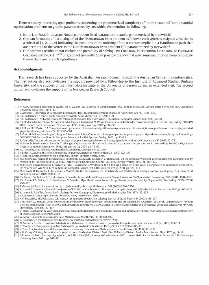
Fig. 1. Example of the reduction fromMulticolor Clique to List Coloring.

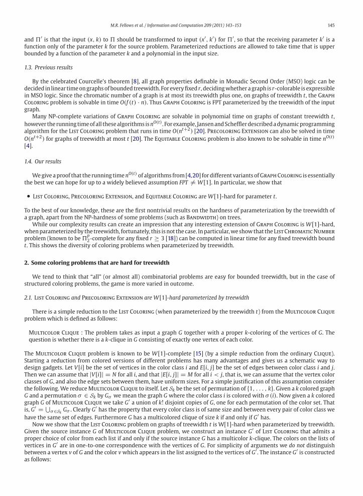
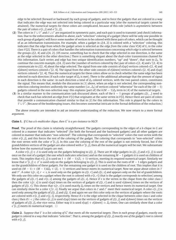
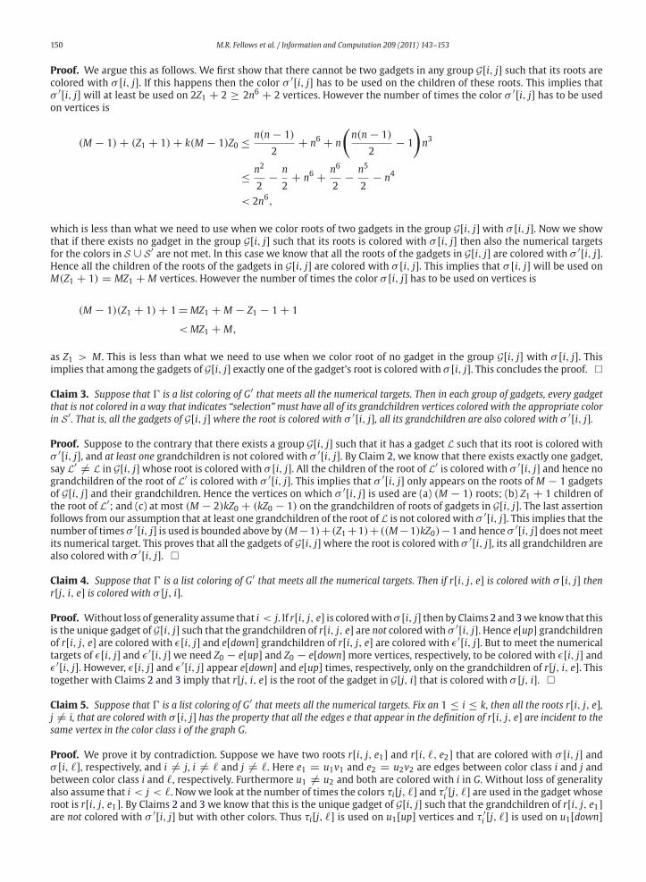
1. There are k vertices v[i] in G′, i = 1, . . . , k, one for each color class of G, and the list assigned to v[i] consists of thecolors corresponding to the vertices in G of color i that is Lv[i] = {V[i]}.

2. For i �= j, there is a degree two vertex in G′ adjacent to v[i] and v[j] for each pair x, y of nonadjacent vertices in G,

where x has color i and y has color j. This vertex is labeled vi,j[x, y] and has {x, y} as its list.This completes the construction. As example of the reduction is shown in Fig. 1. The figure shows an example for the

parameter value k = 4.

The treewidth of G′ is bounded by k as the graph obtained after removing the vertices v[i], 1 ≤ i ≤ k, from G′ is an empty

graph and hence has treewidth 0 (anyway it is well known that degree 2 vertices do not increase the treewidth of a graph).

Now, if G has a multicolor clique K then we can easily list color G′. Assign v[i] with the vertex (color in G′) correspondingto the color class V[i] in the multicolor clique K . Now it is easy to see that every degree 2 vertex in G′ has at least one color

free in its list, as the pair of colors in the list correspond to nonadjacent vertices in G. For the other direction, we show that

the vertices of G, corresponding to the colors assigned to v[i]’s in a list coloring of G′, forms a clique. This follows since two

vertices u and v of G belonging to different color classes do not appear together on a list of some degree 2 vertices in G′ ifand only if they have an edge uv between them in G. This results in the following theorem.

Theorem 1. List Coloring parameterized by treewidth is W[1]-hard.To show that Precoloring Extension is also W[1]-hard when parameterized by treewidth, we reduce from the List

Coloring problem, by simply using many precolored vertices of degree 1 to enforce the lists. This construction does not

increase the treewidth. More precisely given an instance of G = (V, E) of List Coloring we construct an instance G′ ofPrecoloring Extension as follows. Let C = ⋃

v∈V Lv. Now for every vertex v ∈ V , we add � = |C|\|Lv| vertices of degree 1

and make them adjacent to v. Let the set of newly added degree 1 vertices that are adjacent to v be called S(v). We color the

vertices of S(v) with colors in C\Lv where each color is used exactly once. This completes the description of G′, an instance

of Precoloring Extension. Thus we have:

Theorem 2. Precoloring Extension parameterized by treewidth is W[1]-hard.2.2. Equitable Coloring is W[1]-hard parameterized by treewidth

The Equitable Coloring problem is a classical problem with a long history starting from 1960s [19,25]. Bodlaender and

Fomin have shown that determining whether a graph of treewidth at most t admits an equitable coloring, can be solved in

time O(nO(t)) [4].We consider the parameterized complexity of Equitable Coloring (ECP) in graphs with bounded treewidth. We actually

prove a stronger result than the one we have so far stated. We show that when ECP is parameterized by (t, r), where t is

the treewidth bound, and r is the number of color classes, then the problem is W[1]-hard. Before we proceed further we

make remarks on what it means to parameterize by two parameters, say κ1 and κ2. It essentially means parameterizing by

a single parameter k = κ1 + κ2. For an example Independent Set is known to be W[1] complete parameterized by the

solution size k [10], while it is FPT when parameterized by the solution size k and the maximum degree � of the input

graph. That is, there is an algorithm for Independent Set running in time O(f (k + �)nc), where n is the input size. We

refer to [12, Chapter 1, Section 3] for further examples. A combined parameter or two parameters together sometimes

enable a problem to be FPT, while with any one of the parameters they are W[1] hard. For an example Independent Set is

M.R. Fellows et al. / Information and Computation 209 (2011) 143–153 147

not known to be FPT with either the solution size as the parameter or the maximum degree of the input graph. However,

when we show that a problem is W[i]-hard, i ≥ 1, with a combined parameter then it also means that the problem is

W[i]-hard with any one parameter of the combination. Next we show that ECP is W[1]-hard parameterized by (t, r) or

t + r.

In this section, we show a reduction based on a methodology which is sometimes termed as edge representation strategy

for the parameterized reduction fromMulticolor Clique. This strategy is very basic and is useful for many reductions. Note

that the instance G = (V, E) of Multicolor Clique has its vertices colored by the integers 1, ..., k. Let V[i] denote the set

of vertices of color i, and let E[i, j], for 1 ≤ i < j ≤ k, denote the set of edges e = uv, where u ∈ V[i] and v ∈ V[j]. We also

assume that |V[i]| = N for all i, and that |E[i, j]| = M for all i < j, that is, the vertex color classes of G, and also the edge

sets between them, have uniform sizes.

In what follows next we adhere to edge representation strategy and form gadgets in the context of reduction from

Multicolor Clique to Equitable Coloring Problem on graphs with bounded treewidth. To show the desired reduction, we

introduce two intermediate problems.

List Equitable Coloring Problem (LECP): Given an input graph G = (V, E), lists Lv of colors for every vertex v ∈ V and a

positive integer r; does there exist a proper coloring f of G with exactly r colors that for every vertex v ∈ V uses a color

from its list Lv such that for any two color class, Vi and Vj of the coloring f , ||Vi| − |Vj|| ≤ 1?

Number List Coloring Problem (NLCP): Given an input graph G = (V, E), lists Lv of colors for every vertex v ∈ V , a

function h : ∪v∈V Lv → N, associating a number to each color, and a positive integer r; does there exist a proper coloring

f of G with r colors that for every vertex v ∈ V uses a color from its list Lv, such that any color class Vc of the coloring f is

of size h(c)?

List analogues of equitable coloring have been previously studied by Kostochka et al. [22]. Our main effort is in the

reduction of theMulticolor Clique problem to NLCP.

We will use the following sets of colors in our construction of an instance of NLCP:

1. S = {σ [i, j] : 1 ≤ i �= j ≤ k}2. S ′ = {σ ′[i, j] : 1 ≤ i �= j ≤ k}3. T = {τi[r, s] : 1 ≤ i ≤ k, 1 ≤ r < s ≤ k, r �= i, s �= i}4. T ′ = {τ ′

i [r, s] : 1 ≤ i ≤ k, 1 ≤ r < s ≤ k, r �= i, s �= i}5. E = {ε[i, j] : 1 ≤ i < j ≤ k}6. E ′ = {ε′[i, j] : 1 ≤ i < j ≤ k}.

Note that |S| = |S ′| = 2(k

2

), that is, there are distinct colors σ [2, 3] and σ [3, 2], etc. In contrast, the colors τi[r, s] are

only defined for r < s.

WeassociatewitheachvertexandedgeofG apair of (unique) identificationnumbers. Theup-identificationnumber v[up] fora vertex v should be in the range [n2 +1, n2 +n], if G has n vertices and it could be chosen arbitrarily, but uniquely. Similarly,

the up-identification number e[up] of an edge e ofG can be assigned (arbitrarily, but uniquely) in the range [2n2+1, 2n2+m],assuming G has m edges.

Choose a suitably large positive integer Z0, for example Z0 = n3, and define the down-identification number v[down] for avertex v to be Z0 − v[up], and similarly for the edges e of G, define the down-identification number e[down] to be Z0 − e[up].

Choose a second large positive integer, Z1 >> Z0, for example, we may take Z1 = n6.

Next we describe various gadgets and the way they are combined in the reduction. First we describe the gadget which

encodes the selection of the edge going between two particular color classes in G. In other words, we will think of the

representation of a k-clique in G as involving the selection of edges (with each edge selected twice, once in each direction)

between the color classes of vertices in G, with gadgets for selection, and to check two things: (1) that the selections in

opposite color directions match, and (2) that the edges chosen from color class V[i] going to V[j] (for various j �= i) all

emanate from the same vertex in V[i].There are 2

(k

2

)groups of gadgets, one for each pair of color indices i �= j. If 1 ≤ i < j ≤ k, then we will refer to the

gadgets in the group G[i, j] as forward gadgets, and we will refer to the gadgets in the group G[j, i] as backward gadgets.

If e ∈ E[i, j], then there is one forward gadget corresponding to e in the group G[i, j], and one backward gadget corre-

sponding to e in the group G[j, i]. The construction of these gadgets is described as follows:

2.2.1. The forward gadget corresponding to e = uv ∈ E[i, j]The gadget has a root vertex r[i, j, e], and consists of a tree of height 2. The list assigned to this root vertex contains

two colors: σ [i, j] and σ ′[i, j]. The root vertex has Z1 + 1 children, and each of these is also assigned the two-element list

containing the colors σ [i, j] and σ ′[i, j]. One of the children vertices is distinguished, and has 2k groups of further children:

148 M.R. Fellows et al. / Information and Computation 209 (2011) 143–153

• e[up] children assigned the list {σ ′[i, j], ε[i, j]}.• e[down] children assigned the list {σ ′[i, j], ε′[i, j]}.• For each r in the range j < r ≤ k, u[up] children assigned the list {σ ′[i, j], τi[j, r]}.• For each r in the range j < r ≤ k, u[down] children assigned {σ ′[i, j], τ ′

i [j, r]}.• For each r in the range 1 ≤ r < j, u[down] children assigned {σ ′[i, j], τi[r, j]}.• For each r in the range 1 ≤ r < j, u[up] children assigned the list {σ ′[i, j], τ ′i [r, j]}.

Thus the number of grandchildren of r[i, j, e] ise[up] + e[down] + (k − j)u[up] + (k − j)u[down] + (j − 1)u[down] + (j − 1)u[up]

= Z0 + (k − j)Z0 + (j − 1)Z0

= kZ0.

2.2.2. The backward gadget corresponding to e = uv ∈ E[i, j]The gadget has a root vertex r[j, i, e], and consists of a tree of height 2. The list assigned to this root vertex contains

two colors: σ [j, i] and σ ′[j, i]. The root vertex has Z1 + 1 children, and each of these is also assigned the two-element list

containing the colors σ [j, i] and σ ′[j, i]. One of the children vertices is distinguished, and has 2k groups of further children:

• e[up] children assigned the list {σ ′[j, i], ε′[i, j]}.• e[down] children assigned the list {σ ′[j, i], ε[i, j]}.• For each r in the range i < r ≤ k, v[up] children assigned the list {σ ′[j, i], τj[i, r]}.• For each r in the range i < r ≤ k, v[down] children assigned {σ ′[j, i], τ ′

j [i, r]}.• For each r in the range 1 ≤ r < i, v[down] children assigned {σ ′[j, i], τj[r, i]}.• For each r in the range 1 ≤ r < i, v[up] children assigned the list {σ ′[j, i], τ ′j [r, i]}.

Thus the number of grandchildren of r[j, i, e] ise[up] + e[down] + (k − i)v[up] + (k − i)v[down] + (i − 1)v[down] + (i − 1)v[up]

= Z0 + (k − i)Z0 + (i − 1)Z0

= kZ0.

2.2.3. The numerical targets (function h)

1. For all c ∈ (T ∪ T ′), h(c) = Z0.

2. For all c ∈ (E ∪ E ′), h(c) = Z0.

3. For all c ∈ S , h(c) = (M − 1)(Z1 + 1) + 1.

4. For all c ∈ S ′, h(c) = (M − 1) + (Z1 + 1) + k(M − 1)Z0.

Given the source instance G of Multicolor Clique problem, we construct an instance G′ of NLCP that admits a proper

choice of color from each list as well as that each color c appears on exactly h(c) vertices (that is, meets its numerical

requirement) if and only if the source instance G has a multicolor k-clique. The instance G′ is essentially the disjoint union

of the edge gadgets. That is,

G′ = ⋃1≤i �=j≤k

G[i, j].

The h function is defined as above. That completes the formal description of the reduction fromMulticolor Clique to NLCP.

We turn now to some motivating remarks about the design of the reduction.

2.2.4. Remarks on the colors, their numerical targets, and their role in the reduction

(1) There are 2(k

2

)groups of gadgets. Each edge of G gives rise to two gadgets. Between any two color classes of G there are

precisely M edges, and therefore M ·(k

2

)edges in G in total. Each group of gadgets therefore contains M gadgets. The

gadgets in each group have two “helper” colors. For example, the group of gadgets G[4, 2] has the helper colors σ [4, 2]and σ ′[4, 2]. The role of the gadgets in this group is to indicate a choice of an edge going from a vertex in the color class

V[4] of G to a vertex in the color class V[2] of G. The role of the 2(k

2

)groups of gadgets is to represent the selection

of(k

2

)edges of G that form a k-clique, with each edge chosen twice, once in each direction. If i < j then the choice is

represented by the coloring of the gadgets in the group G[i, j], and these are the forward gadgets of the edge choice. If

j < i, then the gadgets in G[i, j] are backward gadgets (representing the edge selection in the opposite direction, relative

to the ordering of the color classes of G). The numerical targets for the colors in S ∪ S′ are chosen to force exactly one

M.R. Fellows et al. / Information and Computation 209 (2011) 143–153 149

edge to be selected (forward or backward) by each group of gadgets, and to force the gadgets that are colored in a way

that indicates the edge was not selected into being colored in a particular way (else the numerical targets cannot be

attained). The numerical targets for these colors are complicated, because of this role (which is asymmetric between

the pair of colors σ [i, j] and σ ′[i, j]).(2) The colors in T ∪ T ′ and E ∪ E ′ are organized in symmetric pairs, and each pair is used to transmit (and check) informa-

tion. Due to the enforcements alluded to above, each “selection” coloring of a gadget (there will be only one possible in

each group of gadgets) will force some number of vertices to be coloredwith these pairs of colors, which can be thought

of as an information transmission. For example, when a gadget in G[4, 2] is colored with a “selection” coloring, this

indicates that the edge from which the gadget arises is selected as the edge from the color class V[4] of G, to the color

class V[2]. There is a pair of colors that handles the information transmission concerningwhich edge is selected between

the groups G[2, 4] and G[4, 2]. (Of course, something has to check that the edge selected in one direction, is the same

as the edge selected in the other direction.) There is something elegant about the dual-color transmission channel for

this information. Each vertex and edge has two unique identification numbers, “up” and “down”, that sum to Z0. To

continue the concrete example, G[4, 2] uses the (number of vertices colored by the) pair of colors ε[2, 4] and ε′[2, 4] tocommunicate to G[2, 4] about the edge selected. The signal from one side consists of e[up] vertices colored ε[2, 4] ande[down] vertices colored ε′[2, 4]. The signal from the other side consists of e[down] vertices colored ε[2, 4] and e[up]vertices colored ε′[2, 4]. Thus the numerical targets for these colors allow us to check whether the same edge has been

selected in each direction (if each color target of Z0 is met). There is the additional advantage that the amount of signal

in each direction is the same: in each direction a total of Z0 colored vertices, with the two paired colors, constitutes

the signal. This means that, modulo the discussion in (1) above, when an edge is not selected, the corresponding non-

selection coloring involves uniformly the same number (i.e., Z0) of vertices colored “otherwise” for each of the (M − 1)gadgets colored in the non-selection way: this explains (part of) the k(M − 1)Z0 term in (4) of the numerical targets.

(3) In a similar manner to the communication task discussed above, each of the k − 1 groups of gadgets G[i, _] need to

check that each has selected an edge from V[i] that originates at the same vertex in V[i]. Hence there are pairs of colors

that provide a communication channel similar to that in (2) for this information. This role is played by the colors in

T ∪ T ′. (Because of the bookkeeping issues, this becomes somewhat intricate in the formal definition of the reduction.)

The above remarks are intended to aid an intuitive understanding of the reduction. We now return to a more formal

argument.

Claim 1. If G has a k-multicolor clique, then G′ is a yes-instance to NLCP.

Proof. The proof of this claim is relatively straightforward. The gadgets corresponding to the edges of a k-clique in G are

colored in a manner that indicates “selected” (for both the forward and the backward gadgets) and all other gadgets are

colored in manner that indicates “non-selected”. The coloring that corresponds to “selected” colors the root vertex with the

color σ [i, j], and this forces the rest of the coloring of the gadget. The coloring that corresponds to “non-selected” colors

the root vertex with the color σ ′[i, j]. In this case the coloring of the rest of the gadget is not entirely forced, but if the

grandchildren vertices of the gadget are also coloredwith σ ′[i, j], then all the numerical targets will bemet.We substantiate

below how the numerical targets are met.

A color σ [i, j] ∈ S is used only on the gadgets belonging to G[i, j]. There are M edge gadgets in G[i, j] and σ [i, j] is usedonce on the root of a gadget (the one which indicates selection) and on the remainingM − 1 gadgets it is used on children of

roots. This implies that σ [i, j] is used on 1 + (M − 1)(Z1 + 1) vertices, meeting its required numerical target. Similarly we

know that σ ′[i, j] ∈ S ′ is used only on the gadgets belonging to G[i, j]. This is used on the roots ofM − 1 edges gadgets and

on the grandchildren of these gadgets. For the remaining one gadget it is used on the children of root. This implies that it is

used on (M − 1) + (M − 1)kZ0 + (Z1 + 1) vertices and hence meets its numerical target. Now we argue about colors in Tand T ′. A color τi[r, s], r < s, is used only on the gadgets in G[i, r] and G[i, s] and appears only on the list of grandchildren.

We only use this color on a gadget when the root is colored with σ [i, r] (that is the gadget corresponds to selection) among

the gadgets of G[i, r] and σ [i, s] among the gadgets of G[i, s]. Hence if v is the vertex in the clique from the color class i

then the color τi[r, s] is used v[up] times on the vertices of gadgets of G[i, r] and is used v[down] times on the vertices of

gadgets of G[i, r]. This shows that τi[r, s] is used exactly Z0 times on the vertices and hence meets its numerical target. One

can similarly show for a color τ ′i [r, s]. Finally we argue that colors in E and E ′ meet their numerical target. A color ε[i, j] is

used only among the gadgets of G[i, j] and G[j, i] and again we use this color only on the vertices of gadgets where the roots

are colored with σ [i, j] and σ [j, i], respectively. Hence if e is the edge selected in the clique between color class i and color

class j then if i < j the color ε[i, j] is used e[up] times on the vertices of gadgets of G[i, j] and e[down] times on the vertices

of gadgets of G[i, j], else vice-versa. Either way it is used e[up] + e[down] = Z0 times. One can similarly show that a color

ε′[i, j] meets its numerical target. �

Claim 2. Suppose that is a list coloring of G′ that meets all the numerical targets. Then in each group of gadgets, exactly one

gadget is colored in a way that indicates “selection”. That is, among the gadgets of G[i, j] exactly one of the gadget’s root is coloredwith σ [i, j].

150 M.R. Fellows et al. / Information and Computation 209 (2011) 143–153

Proof. We argue this as follows. We first show that there cannot be two gadgets in any group G[i, j] such that its roots are

colored with σ [i, j]. If this happens then the color σ ′[i, j] has to be used on the children of these roots. This implies that

σ ′[i, j] will at least be used on 2Z1 + 2 ≥ 2n6 + 2 vertices. However the number of times the color σ ′[i, j] has to be used

on vertices is

(M − 1) + (Z1 + 1) + k(M − 1)Z0 ≤ n(n − 1)

2+ n6 + n

(n(n − 1)

2− 1

)n3

≤ n2

2− n

2+ n6 + n6

2− n5

2− n4

< 2n6,

which is less than what we need to use when we color roots of two gadgets in the group G[i, j] with σ [i, j]. Now we show

that if there exists no gadget in the group G[i, j] such that its roots is colored with σ [i, j] then also the numerical targets

for the colors in S ∪ S ′ are not met. In this case we know that all the roots of the gadgets in G[i, j] are colored with σ ′[i, j].Hence all the children of the roots of the gadgets in G[i, j] are colored with σ [i, j]. This implies that σ [i, j] will be used on

M(Z1 + 1) = MZ1 + M vertices. However the number of times the color σ [i, j] has to be used on vertices is

(M − 1)(Z1 + 1) + 1 = MZ1 + M − Z1 − 1 + 1

< MZ1 + M,

as Z1 > M. This is less than what we need to use when we color root of no gadget in the group G[i, j] with σ [i, j]. Thisimplies that among the gadgets of G[i, j] exactly one of the gadget’s root is colored with σ [i, j]. This concludes the proof. �

Claim 3. Suppose that is a list coloring of G′ that meets all the numerical targets. Then in each group of gadgets, every gadget

that is not colored in a way that indicates “selection” must have all of its grandchildren vertices colored with the appropriate color

in S ′. That is, all the gadgets of G[i, j] where the root is colored with σ ′[i, j], all its grandchildren are also colored with σ ′[i, j].Proof. Suppose to the contrary that there exists a group G[i, j] such that it has a gadget L such that its root is colored with

σ ′[i, j], and at least one grandchildren is not colored with σ ′[i, j]. By Claim 2, we know that there exists exactly one gadget,

say L′ �= L in G[i, j] whose root is colored with σ [i, j]. All the children of the root of L′ is colored with σ ′[i, j] and hence no

grandchildren of the root of L′ is colored with σ ′[i, j]. This implies that σ ′[i, j] only appears on the roots of M − 1 gadgets

of G[i, j] and their grandchildren. Hence the vertices on which σ ′[i, j] is used are (a) (M − 1) roots; (b) Z1 + 1 children of

the root of L′; and (c) at most (M − 2)kZ0 + (kZ0 − 1) on the grandchildren of roots of gadgets in G[i, j]. The last assertion

follows from our assumption that at least one grandchildren of the root of L is not colored with σ ′[i, j]. This implies that the

number of times σ ′[i, j] is used is bounded above by (M−1)+ (Z1 +1)+ ((M−1)kZ0)−1 and hence σ ′[i, j] does notmeet

its numerical target. This proves that all the gadgets of G[i, j] where the root is colored with σ ′[i, j], its all grandchildren are

also colored with σ ′[i, j]. �

Claim 4. Suppose that is a list coloring of G′ that meets all the numerical targets. Then if r[i, j, e] is colored with σ [i, j] thenr[j, i, e] is colored with σ [j, i].Proof. Without loss of generality assume that i < j. If r[i, j, e] is coloredwithσ [i, j] then byClaims2 and3weknow that this

is the unique gadget of G[i, j] such that the grandchildren of r[i, j, e] are not colored with σ ′[i, j]. Hence e[up] grandchildrenof r[i, j, e] are colored with ε[i, j] and e[down] grandchildren of r[i, j, e] are colored with ε′[i, j]. But to meet the numerical

targets of ε[i, j] and ε′[i, j] we need Z0 − e[up] and Z0 − e[down] more vertices, respectively, to be colored with ε[i, j] andε′[i, j]. However, ε[i, j] and ε′[i, j] appear e[down] and e[up] times, respectively, only on the grandchildren of r[j, i, e]. Thistogether with Claims 2 and 3 imply that r[j, i, e] is the root of the gadget in G[j, i] that is colored with σ [j, i]. �

Claim 5. Suppose that is a list coloring of G′ that meets all the numerical targets. Fix an 1 ≤ i ≤ k, then all the roots r[i, j, e],j �= i, that are colored with σ [i, j] has the property that all the edges e that appear in the definition of r[i, j, e] are incident to the

same vertex in the color class i of the graph G.

Proof. We prove it by contradiction. Suppose we have two roots r[i, j, e1] and r[i, �, e2] that are colored with σ [i, j] andσ [i, �], respectively, and i �= j, i �= � and j �= �. Here e1 = u1v1 and e2 = u2v2 are edges between color class i and j and

between color class i and �, respectively. Furthermore u1 �= u2 and both are colored with i in G. Without loss of generality

also assume that i < j < �. Nowwe look at the number of times the colors τi[j, �] and τ ′i [j, �] are used in the gadget whose

root is r[i, j, e1]. By Claims 2 and 3 we know that this is the unique gadget of G[i, j] such that the grandchildren of r[i, j, e1]are not colored with σ ′[i, j] but with other colors. Thus τi[j, �] is used on u1[up] vertices and τ ′

i [j, �] is used on u1[down]

M.R. Fellows et al. / Information and Computation 209 (2011) 143–153 151

vertices of the gadget whose root is r[i, j, e1]. Now to meet the numerical requirements of τi[j, �] and τ ′i [j, �] we need to

color more vertices. However these colors can only be given to the vertices of the gadget whose root is r[i, �, e2] and they

need tomeet their numerical requirements by coloring the appropriate number of vertices in this gadget. Thuswe know that

the number of vertices that are assigned the color τi[j, �] and τ ′i [j, �] among the vertices of the gadget rooted at r[i, �, e2]

are u2[down] and u2[up], respectively. Thus the number of times we use τi[j, �] is u1[up] + u2[down] and the number of

times we use τ ′i [j, �] is u1[down] + u2[up]. But u1[up] + u2[down] �= Z0 and u1[down] + u2[up] �= Z0. The last assertion

follows since given an up identification number there is an unique down identification number tomake it equal to Z0. Hence

u1 must be equal to u2, a contradiction to our assumption. Thus all the roots r[i, j, e], j �= i, that are colored with σ [i, j] hasthe property that all the edges e that appear in the definition of r[i, j, e] are incident to the same vertex in the color class i

of the graph G. �

Finally we have the following claim.

Claim 6. Suppose that is a list coloring of G′ that meets all the numerical targets. Then G has a multicolor clique of size k.

Proof. Let F be the set of edges that appears in the gadget whose root r[i, j, e] is colored with σ [i, j] by . First by Claim 2

we know that for every i �= j there is exactly one gadget in G[i, j] whose root is colored with σ [i, j]. By Claim 4 we know

that if e appears in r[i, j, e] then e also appears in r[j, i, e]. Furthermore by Claim 5 we know that all the edges selected in F

whose end-points are colored with i are same. That is, this process only selects a vertex from a color class i and all the edges

emanate from the same vertex. All this shows that the edges in F form a clique in G. �

Now using Claims 1 and 6 we obtain the following.

Theorem 3. NLCP is W[1]-hard for forests, parameterized by the number of colors that appear on the lists.

The reduction from NLCP to LECP is almost trivial, achieved by padding with isolated vertices having single-color lists.

The reduction from LECP to ECP is described as follows. We add a clique on r vertices, numbered from 1 to r. We connect

the vertex i in the clique to all vertices that do not contain i in their list of allowed colors. Clearly, any list coloring of G can

be extended to a coloring of G′ by coloring the vertex i of the clique with color i. On the other hand, any coloring of G′ must

color the vertices of the clique with distinct colors. Without loss of generality, the vertex i of the clique is colored with color

i. Then all neighbors of this vertex, that is, all vertices of G that do not have i in its list, cannot be colored with i. Since G′ is aforest, the treewidth of the resulting graph is at most r. This proves the following theorem.

Theorem 4. Equitable Coloring is W[1]-hard, parameterized by treewidth.

3. LIST CHROMATIC NUMBER parameterized by treewidth is FPT

The notion of the list chromatic number (also known as the choice number) of a graph was introduced by Vizing [30], and

independently by Erdös, Rubin and Taylor in 1980 [11]. A celebrated result that gave impetus to the area was proved by

Thomassen: every planar graph has list chromatic number at most five [28].

We describe an algorithm for the List Chromatic Number problem that runs in linear time for any fixed treewidth bound

t. Our algorithm employs the machinery of Monadic Second Order logic, due to Courcelle [8] (also [2,6]). At a glance, this

may seem surprising, since there is no obvious way to describe the problem in MSO logic — one would seemingly have to

quantify over all possible list assignments to the vertices of G, and the vocabulary of MSO seems not to provide any way to

do this. We employ a “trick” that was first described (to our knowledge) in [5], with further applications described in [7,14].

The essence of the trick is to construct an auxiliary graph that consists of the original input, augmented with additional

semantic vertices, so that the whole ensemble has — or can safely be assumed to have — bounded treewidth, and relative to

which the problem of interest can be expressed in MSO logic.

A list assignment L with |Lv| ≥ r for all v ∈ V is termed an r-list assignment. A list assignment L from which G cannot be

properly colored is called bad. Thus, a graph G does not have list chromatic number χl(G) ≤ r, if and only if there is a bad

r-list assignment for G.

The following lemma is crucial to the approach.

Lemma 1. If a graph of treewidth at most t admits any bad r-list assignment, then it admits a bad list assignment where the

colors are drawn from a set of (2t + 1)r colors.

Proof. First of all, we may note that if G has treewidth bounded by t, then χl(G) ≤ t + 1 (and similarly, the chromatic

number of G is at most t + 1). This follows easily from the inductive definition of t-trees. We can therefore assume that

r ≤ t + 1.

Fix attention on a width t tree decomposition D for G, where the bags of the decomposition are indexed by the tree T .

For a node t of T , let D(t) denote the bag associated to the node t. Suppose that L is a bad r-list assignment for G, and let C

152 M.R. Fellows et al. / Information and Computation 209 (2011) 143–153

denote the union of the lists of L. For a color α ∈ C, let Tα denote the subforest of T induced by the set of nodes t of T for

which D(t) contains a vertex v of G, where the color α occurs in the list Lv. Let T (α) denote the set of trees of the forest Tα .

Let T denote the union of the sets T (α), taken over all of the colors α that occur in the list assignment L:

T = ⋃α∈C

T (α).

We consider that two trees T ′ and T ′′ in T are adjacent if the distance between T ′ and T ′′ in T is at most one. Note that T ′and T ′′ might not be disjoint, so the distance between them can be zero. Let G denote the graph thus defined: the vertices

of G are the subtrees in T and the edges are given by the above adjacency relationship.

Suppose that G can be properly colored by the coloring function c′ : T → C′. We can use such a coloring to describe a

modified list assignment L′[c′] to the vertices of G in the following way: if T ′ ∈ T (α) and c′(T ′) = α′ ∈ C′, then replace

each occurrence of the color α on the lists Lv, for all vertices v that belong to bags D(t), where t ∈ T ′, with the color α′.This specification of L′[c′] is consistent, because for any vertex v such that α ∈ Lv, there is exactly one tree T ′ ∈ T (α)

such that v belongs to a bag indexed by nodes of T ′.Claim 1. If c′ is a proper coloring of G, and L is a bad list assignment for G, then L′[c′] is also a bad list assignment for G.

This follows because the trees in G preserve the constraints expressed in having a given color on the lists of adjacent

vertices of G, while the new colors α′ can only be used on two different trees T ′ and T ′′ when the vertices of G in the bags

associated with these trees are at a distance of at least two in G.

Claim 2. The graph G has treewidth at most 2(t + 1)r − 1.

A tree decomposition D′ for G of width at most 2(t + 1)r can be described as follows. Subdivide each edge tt′ of T with

a node of degree two denoted s(t, t′). Assign to each node t the bag D′(t) consisting of those trees T ′ of G that include t.

There are at most (t + 1)r such trees. Assign to each node s(t, t′) the bag D′(s(t, t′)) = D′(t) ∪ D′(t′). It is straightforward

to verify that this satisfies the requirements of a tree decomposition for G.The lemma now follows from the fact that G can be properly colored with 2(t + 1)r colors. �

Theorem5. The List ChromaticNumberproblem, parameterized by the treewidth bound t, is fixed-parameter tractable, solvable

in linear time for every fixed t.

Proof. The algorithm consists of the following steps:

Step 1. Compute in linear time, using Bodlaender’s algorithm, a tree-decomposition for G of width at most t. Consider the

vertices of G to be of type 1.

Step 2. Introduce 2(t + 1)r new vertices of type 2, and connect each of these to all vertices of G. The treewidth of this

augmented graph is at most t + 2(t + 1)r = O(t2).Step 3. The problem can nowbe expressed inMSO logic. That this is so, is not entirely trivial, and is argued as follows (sketch).

We employ a routine extension of MSO logic that provides predicates for the two types of vertices.

IfG admits a bad r-list assignment, then this is witnessed by a set of edges F between vertices ofG (that is, type 1 vertices)

and vertices of type 2 (that represent the colors), such that every vertex v of G has degree r relative to F . Thus, the r incident

F-edges represent the colors of Lv. It is routine to assert the existence of such a set of edges in MSO logic.

The property that such a set of edges F represents a bad list assignment can be expressed as: “For every subset F ′ ⊂ F

such that every vertex of G has degree 1 relative to F ′ (and thus, F ′ represents a choice of a color for each vertex, chosen from

its list), there is an adjacent pair of vertices u and v of G, such that the represented color choice is the same, i.e., u and v are

adjacent by edges of F ′ to the same type 2 (color-representing) vertex.” The translation of this statement into formal MSO is

routine. �

4. Conclusion and open problems

Structured optimization problems, such as the coloring problems considered here, have strong claims with respect to

applications. A source of discussion of these applications is the recent dissertation of Marx [24]. It seems interesting and

fruitful to consider such problems from the parameterized point of view, and to investigate how such extra problem structure

(which tends to increase both computational complexity, and real-world applicability) interacts with parameterizations

(such as bounded treewidth), that frequently lead to tractability.

The outcome of the investigation here of some well-known locally or globally constrained coloring problems has turned

up a few surprises: first of all, that the List Chromatic Number problem is actually FPT, whenwe parameterize by treewidth.

It is also somewhat surprising that this good news does not extend to List Coloring, Precoloring Extension or Equitable

Coloring, all of which turn out to be hard forW[1]. Results of the preliminary version of this paper [13] have led to thorough

investigations of structural parameterizations like treewidth or clique-width [9,16,17,27].

M.R. Fellows et al. / Information and Computation 209 (2011) 143–153 153

There aremany interesting open problems concerning the parameterized complexity of “more structured” combinatorial

optimization problems on graphs, parameterized by treewidth. We mention the following:

1. Is the List Edge Chromatic Number problem fixed-parameter tractable, parameterized by treewidth?

2. One can formulate a “list analogue” of the Hamiltonian Path problem as follows: each vertex is assigned a list that is

a subset of {1, 2, ..., n} indicating the positions in the ordering of the n vertices implicit in a Hamiltonian path that

are permitted to the vertex. Is the List Hamiltonian Path problem FPT, parameterized by treewidth?

3. Our hardness results do not exclude the possibility of solving List Coloring, Precoloring Extension, or Equitable

Coloring in time f (t)·no(t) ongraphs of treewidth t. Is it possible to show that up to someassumption fromcomplexity

theory there are no such algorithms?

Acknowledgments

This research has been supported by the Australian Research Council through the Australian Centre in Bioinformatics.

The first author also acknowledges the support provided by a Fellowship to the Institute of Advanced Studies, Durham

University, and the support of the Informatics Institute at the University of Bergen during an extended visit. The second

author acknowledges the support of the Norwegian Research Council.

References

[1] N. Alon, Restricted colorings of graphs, in: K. Walker (Ed.), Surveys in Combinatorics 1993, London Math. Soc. Lecture Notes Series, vol. 187, Cambridge

University Press, 1993, pp. 1–33.

[2] S. Arnborg, J. Lagergren, D. Seese, Easy problems for tree-decomposable graphs, Journal of Algorithms 12 (1991) 308–340.[3] H.L. Bodlaender, A tourist guide through treewidth, Acta Cybernetica 11 (1993) 1–21.

[4] H.L. Bodlaender, F.V. Fomin, Equitable colorings of bounded treewidth graphs, Theoretical Computer Science 349 (2005) 22–30.[5] H.L. Bodlaender,M. Fellows,M. Langston,M.A. Ragan, F. Rosamond,M.Weyer, Quadratic kernelization for convex recoloring of trees, in: Proceedings COCOON

2007, Lecture Notes in Computer Science, vol. 4598, Springer-Verlag, 2007, pp. 86–96.[6] R.B. Borie, R.G. Parker, C.A. Tovey, Automatic generation of linear-time algorithms from predicate calculus descriptions of problems on recursively generated

graph families, Algorithmica 7 (1992) 555–581.

[7] B. Chor,M. Fellows,M.A. Ragan, I. Razgon, F. Rosamond, S. Snir, Connected coloring completion for general graphs: algorithms and complexity, in: ProceedingsCOCOON 2007, Lecture Notes in Computer Science, vol. 4598, Springer-Verlag, 2007, pp. 75–85.

[8] B. Courcelle, The monadic second-order logic of graphs I: recognizable sets of finite graphs, Information and Computation 85 (1990) 12–75.[9] M. Dom, D. Lokshtanov, S. Saurabh, Y. Villanger, Capacitated domination and covering: a parameterized perspective, in: Proceedings IWPEC 2008, Lecture

Notes in Computer Science, vol. 5018, Springer-Verlag, 2008, pp. 78–90.[10] R.G. Downey, M.R. Fellows, Parameterized Complexity, Springer-Verlag, 1999.

[11] P. Erdös, A.L. Rubin, H. Taylor, Choosability in graphs, Congressus Numerantium 26 (1980) 122–157.[12] J. Flum, M. Grohe, Parameterized Complexity Theory, Springer-Verlag, 2006.

[13] M. Fellows, F.V. Fomin, D. Lokshtanov, F. Rosamond, S. Saurabh, S. Szeider, C. Thomassen, On the complexity of some colorful problems parameterized by

treewidth, in: Proceedings COCOA 2007, Lecture Notes in Computer Science, vol. 4616, Springer-Verlag, 2007, pp. 366–377.[14] M. Fellows, P. Giannopoulos, C. Knauer, C. Paul, F. Rosamond, S. Whitesides, N. Yu, Milling a graph with turn costs: a parameterized complexity perspective,

in: Proceedings WG 2010, Lecture Notes in Computer Science, vol. 6410, Springer-Verlag, 2010, pp. 123–134.[15] M. Fellows, D. Hermelin, F. Rosamond, S. Vialette, On the fixed-parameter intractability and tractability of multiple-interval graph properties, Theoretical

Computer Science 410 (2009) 53–61.[16] F.V. Fomin, P.A. Golovach, D. Lokshtanov, S. Saurabh, Intractability of Clique-width Parameterizations, SIAM Journal on Computing 39 (5) (2010) 1941–1956.

[17] F.V. Fomin, P.A. Golovach, D. Lokshtanov, S. Saurabh, Algorithmic lower bounds for problems parameterized by Clique-width, Proceedings SODA (2010)

493–502.[18] S. Gutner, M. Tarsi, Some results on (a : b)-choosability, Discrete Mathematics 309 (2009) 2260–2270.

[19] A. Hajnal, E. Szemerédi, Proof of a conjecture of P. Erdos, in: Combinatorial Theory and its Applications, vol. II, North-Holland, Amsterdam, 1970, pp. 601–623.[20] K. Jansen, P. Scheffler, Generalized colorings for tree-like graphs, Discrete Applied Mathematics 75 (1997) 135–155.

[21] T.R. Jensen, B. Toft, Graph Coloring Problems, Wiley Interscience, 1995.[22] A.V. Kostochka, M.J. Pelsmajer, D.B. West, A list analogue of equitable coloring, Journal of Graph Theory 44 (2003) 166–177.

[23] J. Kratochvil, Z. Tuza, M. Voigt, New trends in the theory of graph colorings: choosability and list coloring, in: R. Graham (Ed.), et al., Contemporary Trends in

Discrete Mathematics (from DIMACS and DIMATIA to the Future), DIMACS Series in Discrete Mathematics and Theoretical Computer Science, vol. 49, AMS,Providence, 1999, pp. 183–197.

[24] D. Marx, Graph coloring with local and global constraints, Department of Computer Science and Information Theory, Ph.D. dissertation, Budapest Universityof Technology and Economics, 2004.

[25] W. Meyer, Equitable coloring, American Mathematical Monthly 80 (1973) 920–922.[26] R. Niedermeier, Invitation to Fixed Parameter Algorithms, Oxford University Press, 2006.

[27] M. Samer, S. Szeider, Constraint satisfaction with bounded treewidth revisited, Journal of Computer and System Sciences 76 (2) (2010) 103–114.

[28] C. Thomassen, Every planar graph is 5-choosable, Journal of Combinatorial Theory Series B 62 (1994) 180–181.[29] Z. Tuza, Graph colorings with local constraints – a survey, Discussiones Mathematicae – Graph Theory 17 (1997) 161–228.

[30] V.G. Vizing, Coloring the vertices of a graph in prescribed colors. Diskret. Analiz No. 29 Metody Diskret. Anal. v Teorii Kodov i Shem 1976, pp. 3–10.[31] D.R.Woodall, List colourings of graphs, in: J.W.P. Hirschfeld (Ed.), Surveys in Combinatorics 2001, LondonMath. Soc. LectureNotes Series, vol. 288, Cambridge

University Press, 2001, pp. 269–301.