On the Computation of Size-Correct Power-DirectedTests with Null Hypotheses Characterized by

Inequalities∗

Adam McCloskey†

Brown University

November 2013; This Version: March 2015

Abstract

This paper presents theoretical results and a computational algorithm that allows apractitioner to conduct hypothesis tests in nonstandard contexts under which the nullhypothesis is characterized by a finite number of inequalities on a vector of parameters.The algorithm allows one to obtain a test with uniformly correct asymptotic size, whiledirecting power towards alternatives of interest, by maximizing a user-chosen localweighted average power criterion. Existing feasible methods for size control in thiscontext do not allow the user to direct the power of the test toward alternatives ofinterest while controlling size. This is because presently available theoretical resultsrequire the user to search for a maximal empirical quantile over a potentially high-dimensional Euclidean space via repeated Monte Carlo simulation. The theoreticalresults I establish here reduce the space required for this search to a finite number ofpoints for a large class of test statistics and data-dependent critical values, enablingpower-direction to be computationally feasible. The results apply to a wide variety oftesting contexts including tests on parameters in partially-identified moment inequalitymodels and tests for the superior predictive ability of a benchmark forecasting model.I briefly analyze the asymptotic power properties of the new testing algorithm overexisting feasible tests in a Monte Carlo study.

Keywords: composite hypothesis testing, weighted average power, moment in-equalities, partial identification, forecast comparison, monotonicity testing

∗I am grateful to Juan Carlos Escanciano, Kirill Evdokimov, Patrik Guggenberger, Marc Henry, FrancescaMolinari, Jose Luis Montiel Olea, Joseph Romano and Jorg Stoye for helpful comments and to SimonFreyeldenhoven for excellent research assistance. Support from the NSF under grant SES-1357607 is grate-fully acknowledged.†Department of Economics, Brown University, Box B, 64 Waterman St., Providence, RI, 02912

(adam mccloskey@brown.edu, http://www.econ.brown.edu/fac/adam mccloskey/Home.html).

1 Introduction

Hypothesis tests characterized by a finite number of inequalities have appeared in numerous

and varied forms throughout the econometrics literature. Though the contexts may at first

glance appear distinct, examples of tests sharing this feature include tests of inequality

constraints in regression models (Wolak, 1987, 1989, 1991), tests for the superior predictive

ability of a forecasting model (White, 2000; Hansen, 2005; Romano and Wolf, 2005), tests

of monotonicity in expected asset returns (Patton and Timmermann, 2010; Romano and

Wolf, 2013)1 and perhaps the most studied in the present econometrics literature: tests on

parameters in partially identified moment inequality models (e.g., Manski and Tamer, 2002;

Chernozhukov et al., 2007; Bajari et al., 2007; Cilberto and Tamer, 2009; Pakes et al., 2011;

Beresteanu et al., 2011; Galichon and Henry, 2011; Bontemps et al., 2012). This class of

testing problems is nonstandard in the sense that the null hypothesis is composite and the

asymptotic distributions of test statistics used to conduct these tests are discontinuous in

certain parameters allowed under the null.

To increase the power of asymptotically size-controlled tests, a handful of papers have

suggested approaches that use the data to determine which point in the null hypothesis

parameter space the critical values (CVs) ought to be constructed from. More specifically,

these approaches require a tuning parameter that, along with the data, determines how far a

given inequality under the null hypothesis should be set from binding in the construction of

the CV. For example, see Andrews and Soares (2010) in the moment inequality context and

Hansen (2005) in the context of testing for superior predictive ability. These approaches typ-

ically require the tuning parameter to diverge at an appropriate rate to result in a test with

correct asymptotic size. To better account for the uncertainty involved in data-dependent

CV construction, and consequently better control finite sample size, Andrews and Barwick

(2012a) examine an alternative asymptotic approach that does not require such tuning pa-

rameter divergence. An appealing feature of this latter approach is that in theory, it should

allow the user to choose the tuning parameter to maximize a local weighted average power

(WAP) criterion. However, doing so is often computationally infeasible because it requires

the user to search for a maximal empirical quantile over a potentially high-dimensional Eu-

clidean space via repeated Monte Carlo simulation. On the other hand, Romano et al. (2014)

advocate an approach based upon the Bonferroni inequality which also does not assume tun-

1Strictly speaking, the inequality testing framework of this paper applies to a particular form of null andalternative hypotheses for this problem. See Patton and Timmermann (2010) and Romano and Wolf (2013)for details.

1

ing parameter divergence (see also McCloskey, 2012). However, this latter approach can be

conservative, with asymptotic size strictly less than its nominal level and an associated power

loss.

The results presented in this paper simultaneously address three major issues of testing

in these contexts: size-control, power-maximization and computational feasibility. Like An-

drews and Barwick (2012a), I examine a class of test statistics and data-dependent CVs that

allow for the construction of asymptotically size-correct tests that can be designed to maxi-

mize a WAP criterion. However, I establish theoretical results that substantially reduce the

computational burden of test construction by reducing the required search space of maximal

empirical quantiles to a finite set of points. More specifically, for a given tuning parame-

ter, the construction of a valid CV requires the computation of a size-correction factor by

simulating from asymptotic distributions that are determined by whether each inequality

in the null hypothesis is binding or “far” from binding. The number of such distributions

is equal to 2p, where p is the number of inequalities present in the null hypothesis.2 This

contrasts with the existing technology, which would require simulation over an uncountably

infinite number of such distributions in a potentially high-dimensional space. Once the rel-

evant search space is determined for a given test statistic, these results naturally lead to a

straightforward (WAP-maximizing) algorithm for CV construction.

The test statistics and CVs covered by this approach include many that have already

been introduced in various contexts in the literature but also allow for potentially new

constructions. Correspondingly, the results not only make WAP maximization feasible for

existing testing procedures but also allow for power gains over existing approaches. In

testing contexts with a large number of inequalities, even with these new computational

simplifications, WAP maximization may not be feasible. However, the results presented here

enable the feasible construction of tests that are guaranteed to be non-conservative in the

sense of attaining asymptotic size equal to the nominal level for any given tuning parameter.

I show how the theoretical results and corresponding computational testing algorithm can

be applied to a leading example of inequality-based tests: tests of parameters in moment

inequality models. Related approaches include Romano and Shaikh (2008), Rosen (2008),

Andrews and Guggenberger (2009b), Fan and Park (2010), Andrews and Soares (2010),

Canay (2010), Andrews and Barwick (2012a) and Romano et al. (2014). For a small number

of inequalities (four), I compare the local asymptotic power of a test constructed from the

2Technically, the required number of such distributions is 2p − 1. See Theorem SC and the discussionfollowing it.

2

WAP-maximizing algorithm presented in this paper with that of Andrews and Barwick

(2012a), as the latter is generally considered to have the best power properties of those

available in the literature for up to 10 inequalities (and tests of nominal level 5%). For a

large number of inequalities (20), I compare the local asymptotic power of a different test with

that of the new approach advanced by Romano et al. (2014). The power analysis reveals

the potential for substantial power gains by using the new computational simplifications

developed here.

The rest of this paper is organized as follows. Section 2 presents the general class of

inequality testing problems we are interested in here, along with the classes of test statistics

and CVs under study. In Section 3, I provide theoretical results that are instrumental

in the feasible construction of uniformly size-controlled tests. I then provide details for

power direction via the maximization of a WAP criterion in Section 4. A straightforward

computational algorithm is presented there. Section 5 summarizes a brief simulation study

comparing the local asymptotic power of two newly feasible testing procedures with the

existing procedures of Andrews and Barwick (2012a) and Romano et al. (2014). Technical

proofs are contained in a mathematical appendix and figures are collected at the end of the

document. In what follows, ∞p denotes (∞, . . . ,∞) with p entries, R+,∞ ≡ R+ ∪ ∞,Rp

+,∞ ≡ R+,∞ × . . . × R+,∞ with the cross-product taken p times, R+∞ ≡ R ∪ ∞ and

Rp+∞ ≡ R+∞ × . . .× R+∞. Finally, I use the convention that Y +∞ = ∞ with probability

(wp) 1 for any random variable Y .

2 Class of Testing Problems

In this paper we are interested in testing null hypotheses for which a parameter vector

satisfies a set of inequalities. Formally, the null hypothesis is defined as

H0 : γ1 ≥ 0, (1)

where γ1 ∈ Rp and the inequality in (1) is meant to be taken element-by-element. In

typical applications, γ1 is (a normalized version of) a vector of moments of a function of an

underlying random vector W for which we observe the realizations Wini=1. For example, γ1

is a normalized version of EF [m(Wi)], where F denotes the probability measure generating

the data and m is a vector-valued function that is measurable with respect to F .

3

Running Example: Tests on a Parameter in Moment Inequality Models

In a leading example, testing whether a parameter value satisfies the restrictions of a

(partially-identified) moment inequality model, m can also be written as a function of an

underlying (finite-dimensional) parameter θ so that the null hypothesis takes the form (1),

where γ1,j is equal to EF [mj(Wi; θ0)]/σj for j = 1, . . . , p, mj(·, θ) are known real-valued

moment functions, Wi are i.i.d. or stationary random vectors with joint distribution F and

σ2j = VarF (mj(Wi; θ0)) (see e.g., Andrews and Soares, 2010; Andrews and Barwick, 2012a;

Romano et al., 2014). We have a sample of i = 1, . . . , n observations of Wi.

2.1 Test Statistics

Testing hypotheses of the form (1) typically proceeds by constructing a test statistic Tn and

examining its asymptotic behavior under H0. In this context, a complication arises from

the fact that the asymptotic distribution of the test statistics used for this type of problem

(see the following subsection for examples) is discontinuously nonpivotal, depending upon

which of the elements of γ1 are equal to zero and which are not. When coupled with

a CV, in order to establish the asymptotic size of the resulting test, one approach is to

examine the test statistic’s behavior under appropriate drifting sequences of distributions

(see e.g., Andrews and Guggenberger, 2009a, 2010; Andrews et al., 2011). More specifically,

the relevant drifting sequences of distributions are characterized asymptotically by a vector of

parameters γn = (γ1,n, γ2,n) such that n1/2γ1,n → h1 ∈ H1 ≡ Rp+,∞ and γ2,n → h2 ∈ H2, where

γ2,n is a correlation matrix and H2 is the closure of a set of correlation matrices. Let γn,h

denote a sequence with this characterization. Under sequences of distributions characterized

by γn,h and H0, we then obtain weak convergence: Tnd−→ Wh, where Wh is a random variable

that is completely characterized by the parameter h ≡ (h1, h2) ∈ H1 ×H2 ≡ H.

It is well known that under the γn,h drifting sequences of distributions, h1 cannot be

consistently estimated. Nevertheless, by replacing population quantities with their finite

sample counterparts, one can inconsistently “estimate” h1 by some h1 such that h1d−→

h1 +N (0p, h2) and consistently estimate h2 by some h2 such that h2p−→ h2 under any γn,h.

The test statistics I focus on are functions of this natural localization parameter estimate,

i.e., Tn = S(h) for some non-negative-valued function S, where h = (h1, h2). Though not

typically written this way, this is in fact true of the majority of test statistics for tests of (1)

found in the literature. The test function corresponding to the modified method of moments

(MMM) statistic considered by Chernozhukov et al. (2007), Romano and Shaikh (2008, 2010),

4

Andrews and Guggenberger (2009b) and Andrews and Soares (2010) in moment-inequality

testing contexts is one such example:

Tn = S(h) =

p∑j=1

[h1,j]2−, where [x]− ≡ x1(x < 0). (2)

Other leading examples of such test functions include weighted versions of the MMM test

function and the test function corresponding to the minimum statistic (min-stat) considered

by White (2000), Hansen (2005) and Romano et al. (2014):3

Tn = S(h) = −min minj=1,...,p

h1,j, 0. (3)

In the typical application, we have a continuous S(·) and hd−→ h = (h1 + Z, h2), where

Zd∼ N (0p, h2), so that S(h)

d−→ S(h). This motivates the following assumption.

Assumption TeF. For any h ∈ H, Wh = S(h), for which the following holds:

(i) S : Rp+∞ × H2 → R+ is a continuous function that is non-increasing in its first p

arguments.

(ii) For any h2 ∈ H2, S(x, h2) = 0 if and only if x ∈ Rp+,∞.

(iii) For any x1, . . . , xi−1, xi+1, . . . , xp ∈ R+∞ and h2 ∈ H2, S(x, h2) is constant in xi ∈R+,∞.

The MMM test function, (weighted) variants of MMM (see e.g., Andrews and Soares,

2010) and the min-stat test functions clearly satisfy Assumption TeF. Similar assumptions

have become standard in the moment-inequality literature. Though the quasi-likelihood ratio

(QLR) test function, originally considered for tests of inequality constraints by Kudo (1963),

Wolak (1987, 1989, 1991) and Sen and Silvapulle (2004), can be expressed as a function of

h, it violates Assumption TeF(iii) and is thus not covered by the results of this paper.

Running Example: Tests on a Parameter in Moment Inequality Models

In this problem, h1,j =√nmj(θ0)/σj(θ0) for j = 1, . . . , p, where

mj(θ) = n−1

n∑i=1

mj(Wi; θ) and σ2j (θ) = n−1

n∑i=1

(mj(Wi; θ)− mj(θ))2.

3These papers use a different variation of the statistic as written here. The equivalent formulation of thestatistic is Tn = S(h) = maxmaxj=1,...,p h1,j , 0 when the null hypothesis is reversed, i.e., H0 : γ1 ≤ 0.

5

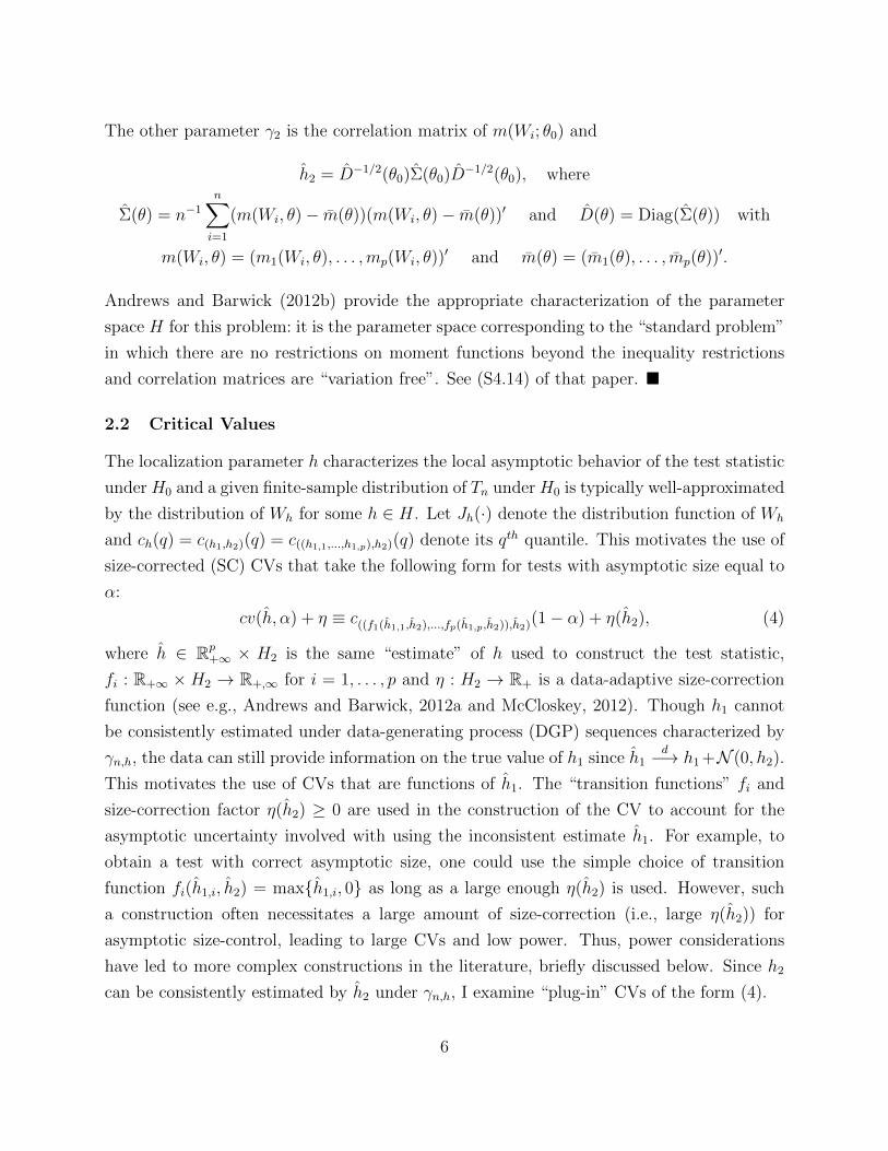
The other parameter γ2 is the correlation matrix of m(Wi; θ0) and

h2 = D−1/2(θ0)Σ(θ0)D−1/2(θ0), where

Σ(θ) = n−1

n∑i=1

(m(Wi, θ)− m(θ))(m(Wi, θ)− m(θ))′ and D(θ) = Diag(Σ(θ)) with

m(Wi, θ) = (m1(Wi, θ), . . . ,mp(Wi, θ))′ and m(θ) = (m1(θ), . . . , mp(θ))

′.

Andrews and Barwick (2012b) provide the appropriate characterization of the parameter

space H for this problem: it is the parameter space corresponding to the “standard problem”

in which there are no restrictions on moment functions beyond the inequality restrictions

and correlation matrices are “variation free”. See (S4.14) of that paper.

2.2 Critical Values

The localization parameter h characterizes the local asymptotic behavior of the test statistic

under H0 and a given finite-sample distribution of Tn under H0 is typically well-approximated

by the distribution of Wh for some h ∈ H. Let Jh(·) denote the distribution function of Wh

and ch(q) = c(h1,h2)(q) = c((h1,1,...,h1,p),h2)(q) denote its qth quantile. This motivates the use of

size-corrected (SC) CVs that take the following form for tests with asymptotic size equal to

α:

cv(h, α) + η ≡ c((f1(h1,1,h2),...,fp(h1,p,h2)),h2)(1− α) + η(h2), (4)

where h ∈ Rp+∞ × H2 is the same “estimate” of h used to construct the test statistic,

fi : R+∞ ×H2 → R+,∞ for i = 1, . . . , p and η : H2 → R+ is a data-adaptive size-correction

function (see e.g., Andrews and Barwick, 2012a and McCloskey, 2012). Though h1 cannot

be consistently estimated under data-generating process (DGP) sequences characterized by

γn,h, the data can still provide information on the true value of h1 since h1d−→ h1 +N (0, h2).

This motivates the use of CVs that are functions of h1. The “transition functions” fi and

size-correction factor η(h2) ≥ 0 are used in the construction of the CV to account for the

asymptotic uncertainty involved with using the inconsistent estimate h1. For example, to

obtain a test with correct asymptotic size, one could use the simple choice of transition

function fi(h1,i, h2) = maxh1,i, 0 as long as a large enough η(h2) is used. However, such

a construction often necessitates a large amount of size-correction (i.e., large η(h2)) for

asymptotic size-control, leading to large CVs and low power. Thus, power considerations

have led to more complex constructions in the literature, briefly discussed below. Since h2

can be consistently estimated by h2 under γn,h, I examine “plug-in” CVs of the form (4).

6

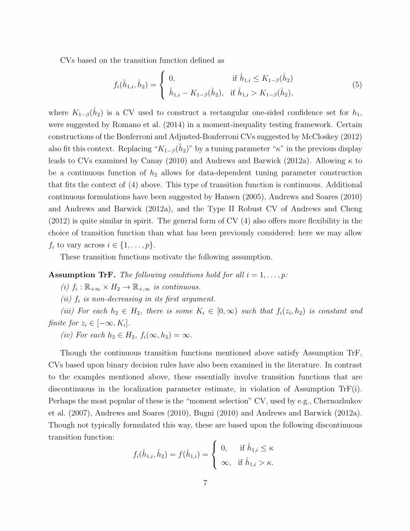
CVs based on the transition function defined as

fi(h1,i, h2) =

0, if h1,i ≤ K1−β(h2)

h1,i −K1−β(h2), if h1,i > K1−β(h2),(5)

where K1−β(h2) is a CV used to construct a rectangular one-sided confidence set for h1,

were suggested by Romano et al. (2014) in a moment-inequality testing framework. Certain

constructions of the Bonferroni and Adjusted-Bonferroni CVs suggested by McCloskey (2012)

also fit this context. Replacing “K1−β(h2)” by a tuning parameter “κ” in the previous display

leads to CVs examined by Canay (2010) and Andrews and Barwick (2012a). Allowing κ to

be a continuous function of h2 allows for data-dependent tuning parameter construction

that fits the context of (4) above. This type of transition function is continuous. Additional

continuous formulations have been suggested by Hansen (2005), Andrews and Soares (2010)

and Andrews and Barwick (2012a), and the Type II Robust CV of Andrews and Cheng

(2012) is quite similar in spirit. The general form of CV (4) also offers more flexibility in the

choice of transition function than what has been previously considered: here we may allow

fi to vary across i ∈ 1, . . . , p.These transition functions motivate the following assumption.

Assumption TrF. The following conditions hold for all i = 1, . . . , p:

(i) fi : R+∞ ×H2 → R+,∞ is continuous.

(ii) fi is non-decreasing in its first argument.

(iii) For each h2 ∈ H2, there is some Ki ∈ [0,∞) such that fi(zi, h2) is constant and

finite for zi ∈ [−∞, Ki].

(iv) For each h2 ∈ H2, fi(∞, h2) =∞.

Though the continuous transition functions mentioned above satisfy Assumption TrF,

CVs based upon binary decision rules have also been examined in the literature. In contrast

to the examples mentioned above, these essentially involve transition functions that are

discontinuous in the localization parameter estimate, in violation of Assumption TrF(i).

Perhaps the most popular of these is the “moment selection” CV, used by e.g., Chernozhukov

et al. (2007), Andrews and Soares (2010), Bugni (2010) and Andrews and Barwick (2012a).

Though not typically formulated this way, these are based upon the following discontinuous

transition function:

fi(h1,i, h2) = f(h1,i) =

0, if h1,i ≤ κ

∞, if h1,i > κ.

7

Other examples of “abrupt transition” CVs include those of Hansen (2005) and Fan and

Park (2010).

Finally, least-favorable CVs (see e.g., Andrews and Guggenberger, 2009a, 2009b), corre-

sponding here to fi(zi) = 0 for all zi ∈ R∞ and i = 1, . . . , p, violate Assumption TrF(iv).

These CVs do not adapt to the data through a transition function and lead to conservative

inference when some elements of γ1 are large and positive. Nevertheless, it is straightforward

to show that the results of Theorem SC below still hold for these CVs but H1 (defined in

the theorem) need only contain the single point 0p.

3 Theoretical Results for Test Implementation

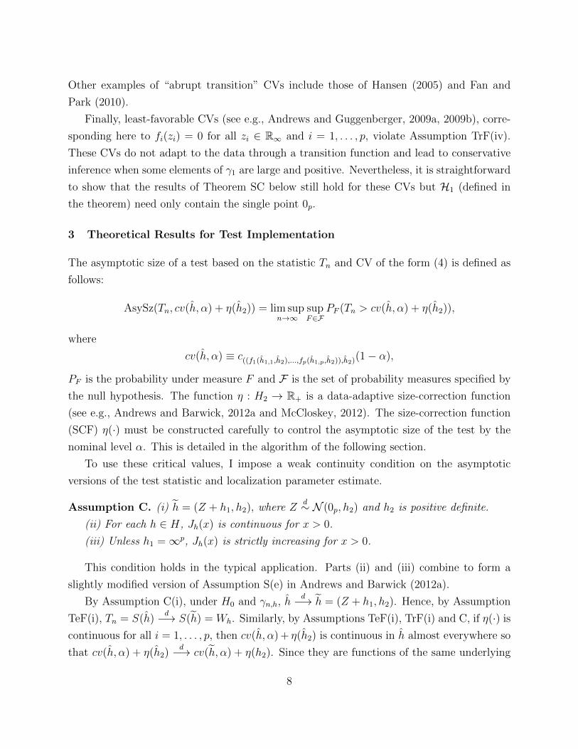
The asymptotic size of a test based on the statistic Tn and CV of the form (4) is defined as

follows:

AsySz(Tn, cv(h, α) + η(h2)) = lim supn→∞

supF∈F

PF (Tn > cv(h, α) + η(h2)),

where

cv(h, α) ≡ c((f1(h1,1,h2),...,fp(h1,p,h2)),h2)(1− α),

PF is the probability under measure F and F is the set of probability measures specified by

the null hypothesis. The function η : H2 → R+ is a data-adaptive size-correction function

(see e.g., Andrews and Barwick, 2012a and McCloskey, 2012). The size-correction function

(SCF) η(·) must be constructed carefully to control the asymptotic size of the test by the

nominal level α. This is detailed in the algorithm of the following section.

To use these critical values, I impose a weak continuity condition on the asymptotic

versions of the test statistic and localization parameter estimate.

Assumption C. (i) h = (Z + h1, h2), where Zd∼ N (0p, h2) and h2 is positive definite.

(ii) For each h ∈ H, Jh(x) is continuous for x > 0.

(iii) Unless h1 =∞p, Jh(x) is strictly increasing for x > 0.

This condition holds in the typical application. Parts (ii) and (iii) combine to form a

slightly modified version of Assumption S(e) in Andrews and Barwick (2012a).

By Assumption C(i), under H0 and γn,h, hd−→ h = (Z + h1, h2). Hence, by Assumption

TeF(i), Tn = S(h)d−→ S(h) = Wh. Similarly, by Assumptions TeF(i), TrF(i) and C, if η(·) is

continuous for all i = 1, . . . , p, then cv(h, α) + η(h2) is continuous in h almost everywhere so

that cv(h, α) + η(h2)d−→ cv(h, α) + η(h2). Since they are functions of the same underlying

8

random vector h, joint convergence of Tn and cv(h, α) + η(h2) follows. Hence under H0

and γn,h, the asymptotic probability of rejecting H0 is P (S(h) > cv(h, α) + η(h2)). Using

arguments found in, inter alia, Andrews and Guggenberger (2010) and Andrews et al. (2011),

this fact allows us to simplify the problem of controlling the asymptotic size of the test to

controlling the asymptotic null rejection probability P (Wh > cv(h, α) +η(h2)) for all h ∈ H,

as described by the following assumption.

Assumption SC. AsySz(Tn, cv(h, α) + η(h2)) = suph∈H P (Wh > cv(h, α) + η(h2))

Assumption SC can be verified in specific applications via the following more primi-

tive condition that is ensured to hold by proper construction of the SCF. It is similar to

Assumptions η1 and η3 of Andrews and Barwick (2012a) and η(i)-(ii) of McCloskey (2012).

Assumption η. (i) η(·) is continuous and

(ii) suph∈H P (Wh > cv(h, α) + η(h2)) = suph∈H limx↓0 P (Wh > cv(h, α) + η(h2)− x).

Part (i) holds by proper construction of the SCF and part (ii) is an unrestrictive conti-

nuity condition. Since Wh = S(h), the left-hand and right-hand side quantities inside the

probabilities of Assumption η(ii) are very different continuous nonlinear functions of the

Gaussian random vector h under Assumption C(i). This implies that, with the exception of

the degenerate case which occurs when h1 =∞p, the left-hand and right-hand side quantities

are equal with probability zero. So long as η is constructed appropriately, these probabilities

will never be maximized at an h for which h1 =∞p, implying that part (ii) holds.4

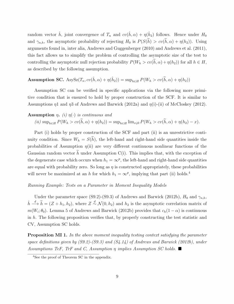
Running Example: Tests on a Parameter in Moment Inequality Models

Under the parameter space (S9.2)-(S9.3) of Andrews and Barwick (2012b), H0 and γn,h,

hd−→ h = (Z + h1, h2), where Z

d∼ N (0, h2) and h2 is the asymptotic correlation matrix of

m(Wi; θ0). Lemma 5 of Andrews and Barwick (2012b) provides that ch(1−α) is continuous

in h. The following proposition verifies that, by properly constructing the test statistic and

CV, Assumption SC holds.

Proposition MI 1. In the above moment inequality testing context satisfying the parameter

space definitions given by (S9.2)-(S9.3) and (S4.14) of Andrews and Barwick (2012b), under

Assumptions TeF, TrF and C, Assumption η implies Assumption SC holds.

4See the proof of Theorem SC in the appendix.

9

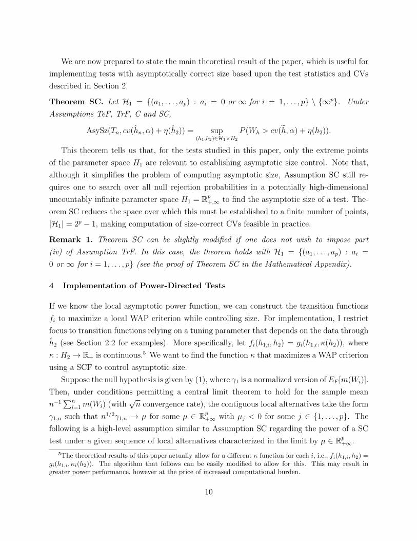
We are now prepared to state the main theoretical result of the paper, which is useful for

implementing tests with asymptotically correct size based upon the test statistics and CVs

described in Section 2.

Theorem SC. Let H1 = (a1, . . . , ap) : ai = 0 or ∞ for i = 1, . . . , p \ ∞p. Under

Assumptions TeF, TrF, C and SC,

AsySz(Tn, cv(hn, α) + η(h2)) = sup(h1,h2)∈H1×H2

P (Wh > cv(h, α) + η(h2)).

This theorem tells us that, for the tests studied in this paper, only the extreme points

of the parameter space H1 are relevant to establishing asymptotic size control. Note that,

although it simplifies the problem of computing asymptotic size, Assumption SC still re-

quires one to search over all null rejection probabilities in a potentially high-dimensional

uncountably infinite parameter space H1 = Rp+,∞ to find the asymptotic size of a test. The-

orem SC reduces the space over which this must be established to a finite number of points,

|H1| = 2p − 1, making computation of size-correct CVs feasible in practice.

Remark 1. Theorem SC can be slightly modified if one does not wish to impose part

(iv) of Assumption TrF. In this case, the theorem holds with H1 = (a1, . . . , ap) : ai =

0 or ∞ for i = 1, . . . , p (see the proof of Theorem SC in the Mathematical Appendix).

4 Implementation of Power-Directed Tests

If we know the local asymptotic power function, we can construct the transition functions

fi to maximize a local WAP criterion while controlling size. For implementation, I restrict

focus to transition functions relying on a tuning parameter that depends on the data through

h2 (see Section 2.2 for examples). More specifically, let fi(h1,i, h2) = gi(h1,i, κ(h2)), where

κ : H2 → R+ is continuous.5 We want to find the function κ that maximizes a WAP criterion

using a SCF to control asymptotic size.

Suppose the null hypothesis is given by (1), where γ1 is a normalized version ofEF [m(Wi)].

Then, under conditions permitting a central limit theorem to hold for the sample mean

n−1∑n

i=1 m(Wi) (with√n convergence rate), the contiguous local alternatives take the form

γ1,n such that n1/2γ1,n → µ for some µ ∈ Rp+∞ with µj < 0 for some j ∈ 1, . . . , p. The

following is a high-level assumption similar to Assumption SC regarding the power of a SC

test under a given sequence of local alternatives characterized in the limit by µ ∈ Rp+∞.

5The theoretical results of this paper actually allow for a different κ function for each i, i.e., fi(h1,i, h2) =gi(h1,i, κi(h2)). The algorithm that follows can be easily modified to allow for this. This may result ingreater power performance, however at the price of increased computational burden.

10

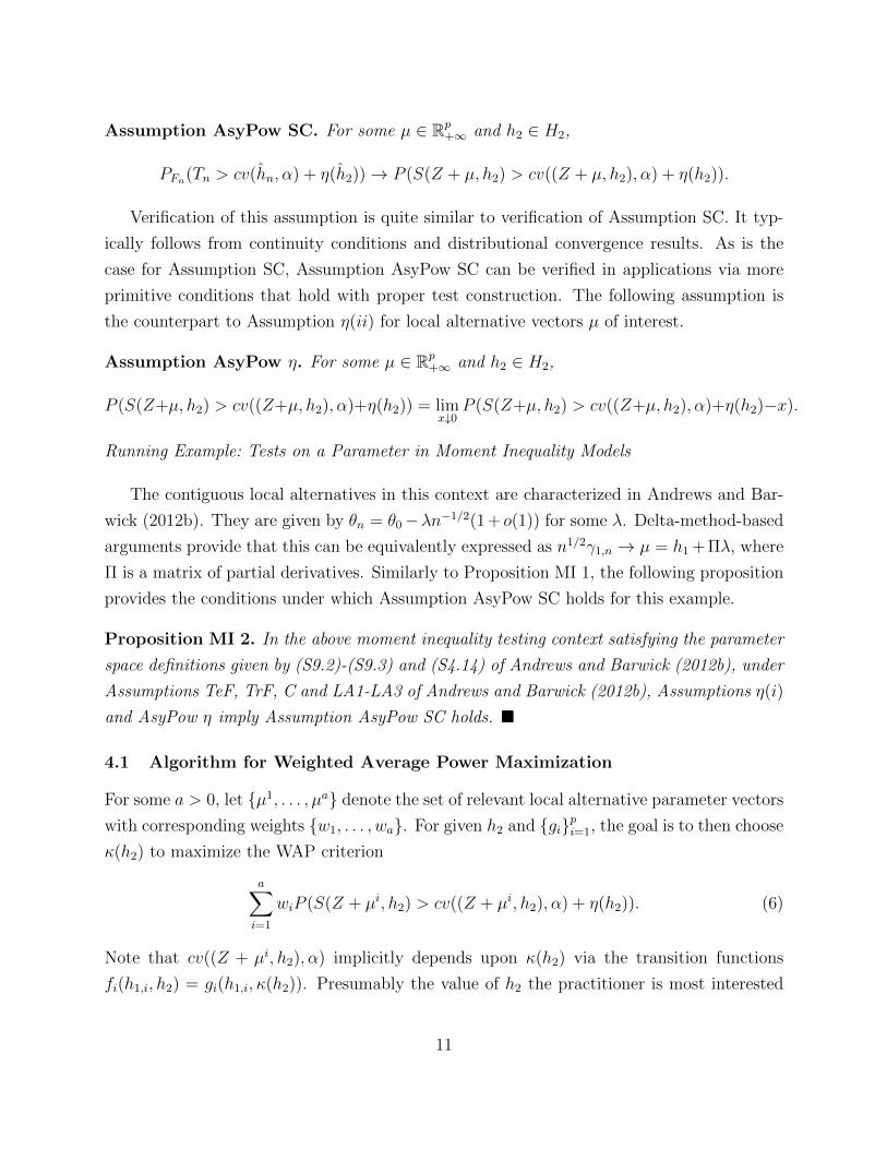
Assumption AsyPow SC. For some µ ∈ Rp+∞ and h2 ∈ H2,

PFn(Tn > cv(hn, α) + η(h2))→ P (S(Z + µ, h2) > cv((Z + µ, h2), α) + η(h2)).

Verification of this assumption is quite similar to verification of Assumption SC. It typ-

ically follows from continuity conditions and distributional convergence results. As is the

case for Assumption SC, Assumption AsyPow SC can be verified in applications via more

primitive conditions that hold with proper test construction. The following assumption is

the counterpart to Assumption η(ii) for local alternative vectors µ of interest.

Assumption AsyPow η. For some µ ∈ Rp+∞ and h2 ∈ H2,

P (S(Z+µ, h2) > cv((Z+µ, h2), α)+η(h2)) = limx↓0

P (S(Z+µ, h2) > cv((Z+µ, h2), α)+η(h2)−x).

Running Example: Tests on a Parameter in Moment Inequality Models

The contiguous local alternatives in this context are characterized in Andrews and Bar-

wick (2012b). They are given by θn = θ0−λn−1/2(1 + o(1)) for some λ. Delta-method-based

arguments provide that this can be equivalently expressed as n1/2γ1,n → µ = h1 + Πλ, where

Π is a matrix of partial derivatives. Similarly to Proposition MI 1, the following proposition

provides the conditions under which Assumption AsyPow SC holds for this example.

Proposition MI 2. In the above moment inequality testing context satisfying the parameter

space definitions given by (S9.2)-(S9.3) and (S4.14) of Andrews and Barwick (2012b), under

Assumptions TeF, TrF, C and LA1-LA3 of Andrews and Barwick (2012b), Assumptions η(i)

and AsyPow η imply Assumption AsyPow SC holds.

4.1 Algorithm for Weighted Average Power Maximization

For some a > 0, let µ1, . . . , µa denote the set of relevant local alternative parameter vectors

with corresponding weights w1, . . . , wa. For given h2 and gipi=1, the goal is to then choose

κ(h2) to maximize the WAP criterion

a∑i=1

wiP (S(Z + µi, h2) > cv((Z + µi, h2), α) + η(h2)). (6)

Note that cv((Z + µi, h2), α) implicitly depends upon κ(h2) via the transition functions

fi(h1,i, h2) = gi(h1,i, κ(h2)). Presumably the value of h2 the practitioner is most interested

11

in is h2 so that construction of the entire function κ(·) is unnecessary in a single given

application.

Choosing a tuning parameter function κ to maximize (6) proceeds similarly to the meth-

ods used to determine the “recommended” moment selection procedure of Andrews and

Barwick (2012a). A key difference here is that Andrews and Barwick (2012a) advocate a

particular data-adaptive tuning parameter function that maximizes a particular WAP cri-

terion (with equal weights), restricting attention to a particular type of transition function

and test function. In contrast, the goal here is to (i) allow for the construction of tests of

size different from 5% and for more than 10 inequalities and (ii) allow the user to specify the

WAP criterion of interest in order to direct power toward alternatives he considers to be the

most relevant to his application. As outlined in the algorithm below, the theoretical results

established here make (i) and (ii) computationally tractable for the first time. Moreover, the

user may choose both the test statistic and transition functions (provided that they satisfy

the relevant assumptions) based upon power and computational tradeoffs, within the context

of his testing problem.

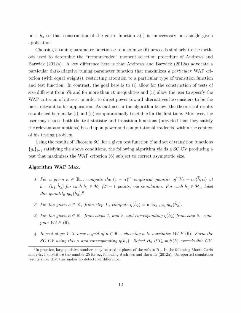
Using the results of Theorem SC, for a given test function S and set of transition functions

gipi=1 satisfying the above conditions, the following algorithm yields a SC CV producing a

test that maximizes the WAP criterion (6) subject to correct asymptotic size.

Algorithm WAP Max.

1. For a given κ ∈ R+, compute the (1 − α)th empirical quantile of Wh − cv(h, α) at

h = (h1, h2) for each h1 ∈ H1 (2p − 1 points) via simulation. For each h1 ∈ H1, label

this quantity ηh1(h2).6

2. For the given κ ∈ R+ from step 1., compute η(h2) ≡ maxh1∈H1 ηh1(h2).

3. For the given κ ∈ R+ from steps 1. and 2. and corresponding η(h2) from step 2., com-

pute WAP (6).

4. Repeat steps 1.-3. over a grid of κ ∈ R+, choosing κ to maximize WAP (6). Form the

SC CV using this κ and corresponding η(h2). Reject H0 if Tn = S(h) exceeds this CV.

6In practice, large positive numbers may be used in places of the∞’s in H1. In the following Monte Carloanalysis, I substitute the number 25 for ∞, following Andrews and Barwick (2012a). Unreported simulationresults show that this makes no detectable difference.

12

Steps 1. and 2. allow one to compute a size-correction η(h2) that uniformly controls the

null rejection probability of the test at h2 for given S, gipi=1 and κ.7 Existing methods of

computation in this context would require one to search over a fine grid of the uncountably

infinite and potentially high-dimensional H1 = Rp+,∞ parameter space to find maximal null

rejection probabilities. More specifically, this would require one to find the smallest η(h2) ≥ 0

such that suph1∈H1P (W(h1,h2) > cv((h1, h2), α)+η(h2)) ≤ α. Steps 3.-4. enables one to choose

κ = κ(h2) to maximize (6) while simultaneously controlling the asymptotic size of the test.

Remark 2. If p is too large, even with the results of this paper, WAP maximization may

become very computationally burdensome since step 1. needs to be repeatedly computed over

2p − 1 points. Nevertheless, steps 1. and 2. can be used to construct size-correct tests for a

given κ ∈ R+, making construction of tests with asymptotic size equal to their nominal level

feasible in many previously infeasible cases. Though the approach of Romano et al. (2014)

allows one to construct asymptotically size-controlled tests when p is large, these tests do not

necessarily have asymptotic size equal to their nominal level. This difference allows the tests

presented here to have power gains over those of Romano et al. (2014) in the large p context.

Remark 3. It is interesting to note that one may also use the results presented in this paper

to compute a non-positive SCF for the CVs used by Romano et al. (2014), provided that

the test function used satisfies Assumption TeF. Adding this non-positive SCF to their CVs

would allow their tests to have size equal to the nominal level, rather than being bounded

above by it.8

5 Local Asymptotic Power Analysis

I now briefly analyze the asymptotic power properties of a test constructed from Algorithm

WAP Max. First, it is instructive to examine how the choice of tuning parameter affects

CV formation and the subsequent power of the test. To fix ideas, let us consider the MMM

test function (2) and CVs constructed using transition function (5) for each i = 1, . . . , p,

replacing K1−β simply with κ ≥ 0. We now graphically analyze SC CVs computed for p = 2

and α = 0.05 at the given value h2 = I2. Figure 1 plots the transition function for two

different κ values, 0.1 and 2, as a function of µ2, where µ2 takes the place of h1,i in (5).

7As mentioned above, the CVs are computed in step 2. only at the point h2 = h2, rather than computingthe entire function η(·), since this is the most relevant point in a given application and h2 is consistent underdrifting γn,h DGPs.

8I thank an anonymous referee for pointing this out.

13

Figure 2 plots the corresponding SC CVs under the local alternative µ = (−1, µ2), as a

function of µ2. That is, Figure 2 graphs cv(((−1, µ2), I2), α) + η(I2) as a function of µ2,

where η(I2) is determined by steps 1. and 2. of Algorithm WAP for each κ = 0.1 and 2. The

underlying localized quantile function that the CVs are constructed from, c((0,µ2),I2)(1− α),

is also included in the figure for comparison. Though the µ values are nonrandom, the graph

provides a heuristic illustration of how the CVs behave under the alternative hypothesis.

We can see that the CV constructed with κ = 2 outperforms that constructed with

κ = 0.1 at either small or large values of µ2 since a smaller CV corresponds to higher power

in the resulting test. Conversely, the CV constructed with κ = 0.1 performs best over an

intermediate range of µ2 values. The features of this specific example generalize to all of

the problems considered in this paper: the power properties of tests based upon SC CVs are

sensitive to the choice of tuning parameter used. Different choices of κ direct power toward

different regions of the alternative hypothesis.

Turning now to local asymptotic power comparison with the test advocated by Andrews

and Barwick (2012a), Figures 3 and 4 graph the local asymptotic power curves for p = 4

and α = 0.05 of (i) SC tests constructed from Algorithm WAP Max using the min-stat

test function (3) and transition function (5), now replacing K1−β(h2) by the “optimal” κ

determined by step 4. of the algorithm; and (ii) Andrews and Barwick’s (2012a) SC test

based upon the QLR test function, moment selection transition functions and a tuning

parameter κ selected to maximize their particular WAP criterion (which was chosen for the

test to have good power over a wide range of alternatives). The local alternatives under

study are characterized by µ = [µ1, 1, 1, 1] with µ1 < 0 and local asymptotic power is

graphed as a function of µ1. Figure 3 corresponds to the correlation matrix h2 = I4 and

Figure 4 corresponds to h2 equal to a Toeplitz matrix with correlations (−0.9, 0.7,−0.5),

as was examined by Andrews and Barwick (2012a). Direct comparison of the power curves

in the figures is not entirely fair because the κ used for power curves (i) are chosen in

Algorithm WAP Max to maximize average power for local alternatives µ = [µ1, 1, 1, 1] with

µ1 ∈ −0.1,−0.2, . . . ,−3.5, precisely the type of alternatives under study, while Andrews

and Barwick’s (2012a) SC test directs power toward a diffuse set of alternatives. Nevertheless,

some interesting results emerge.

First, we can see that gains are possible when the practitioner has a specific type of

alternative in mind. Second, for the correlation matrix used in Figure 4, it is interesting

to note that the relative power performance of tests (i) and (ii) depends on how “far” the

local alternative is from H0, with the min-stat test seeming to perform better for “more

14

local” alternatives. I also made the analogous power comparison for the case of very large

positive correlations with the off-diagonal elements of h2 all equal to 0.9. The results are

omitted for brevity but the power of the directed min-stat test and Andrews and Barwick’s

(2012a) test were very close, with the former tending to be about 0.01 above the latter over

the alternatives under study. In summary, for tests of size α = 0.05 and p = 4 inequalities,

Andrews and Barwick’s (2012a) test performs well, even against directed alternatives, though

significant power gains can be realized.

I conclude with a similar local asymptotic power comparison with the test advocated by

Romano et al. (2014), but now for a large number of inequalities: 20. For this large number

of inequalities, choosing κ to maximize a WAP criterion is computationally expensive. So for

this experiment, I simply set κ = 2 and computed the appropriate SCF via steps 1. and 2. of

Algorithm WAP Max (see Remark 2). Figure 5 graphs the local asymptotic power curves

for p = 20 , h2 = I20 and α = 0.05 of (i) SC tests using the MMM test function (2) and

transition function (5), replacing K1−β(h2) with the number two and (ii) Romano et al.’s

(2014) test based upon the QLR test function (which is asymptotically equivalent to MMM

in this context) and K1−α/10(h2). The local alternatives under study are characterized by

µ = [µ1, 3, . . . , 3] with µ1 < 0 and local asymptotic power is graphed as a function of µ1. Here

we can see that there is potential for very large power gains over the potentially conservative

approach of Romano et al. (2014), which is based upon the Bonferroni inequality. Though

the tuning parameter κ used in the SC test was not chosen to maximize a WAP criterion,

by construction, the SC test has asymptotic size equal to the nominal level of the test. The

test of Romano et al. (2014) may have asymptotic size strictly less than its nominal level,

allowing for potential gains in power by tests with exact asymptotic size.

15

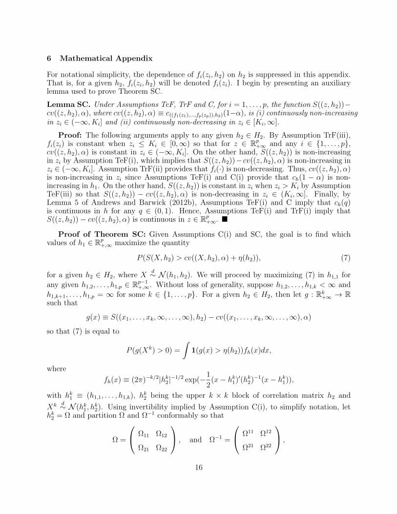
6 Mathematical Appendix

For notational simplicity, the dependence of fi(zi, h2) on h2 is suppressed in this appendix.That is, for a given h2, fi(zi, h2) will be denoted fi(zi). I begin by presenting an auxiliarylemma used to prove Theorem SC.

Lemma SC. Under Assumptions TeF, TrF and C, for i = 1, . . . , p, the function S((z, h2))−cv((z, h2), α), where cv((z, h2), α) ≡ c((f1(z1),...,fp(zp)),h2)(1−α), is (i) continuously non-increasingin zi ∈ (−∞, Ki] and (ii) continuously non-decreasing in zi ∈ [Ki,∞].

Proof: The following arguments apply to any given h2 ∈ H2. By Assumption TrF(iii),fi(zi) is constant when zi ≤ Ki ∈ [0,∞) so that for z ∈ Rp

+∞ and any i ∈ 1, . . . , p,cv((z, h2), α) is constant in zi ∈ (−∞, Ki]. On the other hand, S((z, h2)) is non-increasingin zi by Assumption TeF(i), which implies that S((z, h2))−cv((z, h2), α) is non-increasing inzi ∈ (−∞, Ki]. Assumption TrF(ii) provides that fi(·) is non-decreasing. Thus, cv((z, h2), α)is non-increasing in zi since Assumptions TeF(i) and C(i) provide that ch(1 − α) is non-increasing in h1. On the other hand, S((z, h2)) is constant in zi when zi > Ki by AssumptionTeF(iii) so that S((z, h2)) − cv((z, h2), α) is non-decreasing in zi ∈ (Ki,∞]. Finally, byLemma 5 of Andrews and Barwick (2012b), Assumptions TeF(i) and C imply that ch(q)is continuous in h for any q ∈ (0, 1). Hence, Assumptions TeF(i) and TrF(i) imply thatS((z, h2))− cv((z, h2), α) is continuous in z ∈ Rp

+∞.

Proof of Theorem SC: Given Assumptions C(i) and SC, the goal is to find whichvalues of h1 ∈ Rp

+,∞ maximize the quantity

P (S(X, h2) > cv((X, h2), α) + η(h2)), (7)

for a given h2 ∈ H2, where Xd∼ N (h1, h2). We will proceed by maximizing (7) in h1,1 for

any given h1,2, . . . , h1,p ∈ Rp−1+,∞. Without loss of generality, suppose h1,2, . . . , h1,k < ∞ and

h1,k+1, . . . , h1,p = ∞ for some k ∈ 1, . . . , p. For a given h2 ∈ H2, then let g : Rk+∞ → R

such that

g(x) ≡ S((x1, . . . , xk,∞, . . . ,∞), h2)− cv((x1, . . . , xk,∞, . . . ,∞), α)

so that (7) is equal to

P (g(Xk) > 0) =

∫1(g(x) > η(h2))fh(x)dx,

where

fh(x) ≡ (2π)−k/2|hk2|−1/2 exp(−1

2(x− hk1)′(hk2)−1(x− hk1)),

with hk1 ≡ (h1,1, . . . , h1,k), hk2 being the upper k × k block of correlation matrix h2 and

Xk d∼ N (hk1, hk2). Using invertibility implied by Assumption C(i), to simplify notation, let

hk2 = Ω and partition Ω and Ω−1 conformably so that

Ω =

Ω11 Ω12

Ω21 Ω22

, and Ω−1 =

Ω11 Ω12

Ω21 Ω22

,

16

where Ω11 and Ω11 are scalar and Ω22 and Ω22 are (k − 1) × (k − 1) submatrices. Also, letabs(·) be an operator such that for an arbitrary matrix A, abs(A) is equal to the matrixcomposed of the absolute values of the entries of A.

Since fh(x) is continuously differentiable in h1,1 and∣∣∣∣∂fh(x)

∂h1,1

∣∣∣∣ ≤ Ω11|x1 − h1,1|+ abs(Ω12) abs(Ω−122 )(|x2 − h1,2|, . . . , |xk − h1,k|)′fh(x),

which is (Lebesgue) integrable due to the integrability of |xi − h1,i|fh(x) for all i = 1, . . . , k,application of the dominated convergence and mean value theorems provides that

∂P (g(Xk) > η(h2))

∂h1,1

=

∫1(g(x) > η(h2))

∂fh(x)

∂h1,1

dx

= Ω11

∫1(g(x) > η(h2))

× (x1 − h1,1)− Ω12Ω−122 (x2 − h1,2, . . . , xk − h1,k)

′fh(x)dx

= Ω11E[1(g(Z + hk1) > η(h2))(Z1 − Ω12Ω−122 (Z2, . . . , Zk)

′)]

= Ω11E[1(g((Z + Ω12Ω−122 Z + h1,1, Z + h1)) > η(h2))Z], (8)

where Zd∼ N (0k, h

k2), Z ≡ (Z2, . . . , Zk)

′, h1 ≡ (h1,2, . . . , h1,k)′, Z

d∼ N (0, 1 − Ω12Ω−122 Ω21)

and Z is independent of Z. Since fh(x) is twice continuously differentiable in h1,1 and∣∣∣∣∂2fh(x)

∂h21,1

∣∣∣∣ ≤ Ω11 + (Ω11)2[(x1 − h1,1)− Ω12Ω−122 (x2 − h1,2, . . . , xk − h1,k)

′]2fh(x),

which is integrable due to the integrability of fh(x) and (xi − h1,i)2fh(x) for all i = 1, . . . , k,

another application of the dominated convergence and mean value theorems implies that forany given h1 ∈ Rk−1

+ , (8) is differentiable and thus continuous in h1,1.Letting f(·) denote the multivariate normal pdf of Z and φ(·) denote the standard normal

pdf, note that for a given h1 ∈ Rk−1+ , (8) is equal to

Ω11√1− Ω12Ω−1

22 Ω21

∫ ∫ ∞0

1(g(z + Ω12Ω−122 z + h1,1, z + h1) > η(h2))

× zφ(z/

√1− Ω12Ω−1

22 Ω21)f(z)dzdz

+Ω11√

1− Ω12Ω−122 Ω21

∫ ∫ 0

−∞1(g(z + Ω12Ω−1

22 z + h1,1, z + h1) > η(h2))

× zφ(z/

√1− Ω12Ω−1

22 Ω21)f(z)dzdz

=Ω11√

1− Ω12Ω−122 Ω21

∫f(z)

(∫S+z,h1

(h1,1)

zφ(z/

√1− Ω12Ω−1

22 Ω21)dz

)dz

17

+Ω11√

1− Ω12Ω−122 Ω21

∫f(z)

(∫S−z,h1

(h1,1)

zφ(z/

√1− Ω12Ω−1

22 Ω21)dz

)dz

= Ah1(h1,1)−Bh1

(h1,1),

say, where

S+z,h1

(h1,1) ≡ z ≥ 0 : g(z + Ω12Ω−122 z + h1,1, z + h1) > η(h2),

S−z,h1

(h1,1) ≡ z < 0 : g(z + Ω12Ω−122 z + h1,1, z + h1) > η(h2).

Note that for any hk1 ∈ Rk+, z ∈ Rk−1 and ε ≥ 0, Lemma SC implies that (i) S+

z,h1(h1,1) ⊆

S+z,h1

(h1,1 + ε) and (ii) S−z,h1

(h1,1 + ε) ⊆ S−z,h1

(h1,1).

Case I: for h1 ∈ Rk−1+ given, there is some h∗1,1 > 0 such that E[1(g(Z + Ω12Ω−1

22 Z +

h∗1,1, Z + h1) > η(h2))Z] = 0, i.e., Ah1(h∗1,1) = Bh1

(h∗1,1). Then, for any 0 ≤ h1,1 < h∗1,1,Ah1

(h1,1) ≤ Ah1(h∗1,1) by property (i) since∫

S+z,h1

(h1,1)

zφ(z/

√1− Ω12Ω−1

22 Ω21)dz ≤∫S+z,h1

(h∗1,1)

zφ(z/

√1− Ω12Ω−1

22 Ω21)dz

for all z ∈ Rk−1 and Ω11 ≥ 0 by the positive semi-definiteness of Ω. Similarly, Bh1(h1,1) ≥

Bh1(h∗1,1) by property (ii). Hence, E[1(g(Z + Ω12Ω−1

22 Z + h1,1, Z + h1) > η(h2))Z] ≤ 0 for

any 0 ≤ h1,1 < h∗1,1. An exactly symmetric argument shows that E[1(g(Z + Ω12Ω−122 Z +

h1,1, Z + h1) > η(h2))Z] ≥ 0 for any h∗1,1 < h1,1 < ∞. Hence for any h1 ∈ Rk−1+ , (8) implies

that (7) is continuously non-increasing in h1,1 ∈ [0, h∗1,1] and continuously non-decreasing inh1,1 ∈ [h∗1,1,∞) so that it attains a supremum at either h1,1 = 0 or h1,1 =∞.

Case II: for h1 ∈ Rk−1+ given, there is no h∗1,1 > 0 such that E[1(g(Z+Ω12Ω−1

22 Z+h∗1,1, Z+

h1) > η(h2))Z] = 0. Then, by the continuity of E[1(g(Z + hk1) > η(h2))Z] = E[1(g(Z +

Ω12Ω−122 Z + h1,1, Z + h1) > η(h2))Z] in h1,1, we have either E[1(g(Z + hk1) > η(h2))Z] ≤ 0

for all h1,1 ≥ 0 or E[1(g(Z + h1) > η(h2))Z] ≥ 0 for all h1,1 ≥ 0. In either case (8) impliesthat (7) is continuous and (weakly) monotone in h1,1 ≥ 0, so that it attains a supremum ateither h1,1 = 0 or h1,1 =∞.

The exactly analogous argument can be made for any h1,i with i = 1, . . . , p, implyingthat (7) is maximized at h1 ∈ Rp

+,∞ such that either h1,i = 0 or h1,i = ∞ for i = 1, . . . , p.

Finally, for h1 =∞p, S(h) = S((∞p, h2)) = 0 wp 1 by Assumption TeF(ii) and

cv(h, α) + η(h2) = cv((∞p, α)) + η(h2) = c((∞,...,∞),h2)(1− α) + η(h2) = η(h2) ≥ 0

wp 1 by Asumptions TeF(ii) and TrF(iv) so that P (S(h) > cv(h, α)+ η(h2)) = 0 at h1 =∞p.Thus, using Assumptions C(i) and SC,

AsySz(Tn, cv(hn, α) + η(h2)) = suph∈H

P (S(h) > cv(h, α) + η(h2))

18

= suph∈H

P (S(h)− cv(h, α)− η(h2) > 0)

= sup(h1,h2)∈H1×H2

P (Wh > cv(h, α) + η(h2)).

Proof of Proposition MI 1: The proof is very similar to the proof of Theorem 1(c)in Andrews and Barwick (2012b) and therefore mostly omitted. Let γ = (γ1, γ2). Note

that under any subsequence tn of n for which t1/2n γ1,tn → h1 for some h1 ∈ Rp

+,∞ andγ2,tn → h2 for some h2 ∈ H2, where γ1,tn is a sequence in Rp

+ and γ2,tn is a sequence inH2, Ttn

cv(htn , a(h2,tn))

=

S(htn)

cv(htn , a(h2,tn))

d−→

S(h)

cv(h, a(h2))

=

Wh

cv(h, a(h2))

,

where h = (h1 + Z, h2) with Z ∼ N (0p, h2) by the following facts. The parameter space

restriction (S9.3) of Andrews and Barwick (2012b), provides that htnd−→ h, under a DGP

sequence characterized by γtn. Lemma 5 of Andrews and Barwick (2012b) provides thatch(1 − α) is continuous in h for all α ∈ (0, 1). Hence, cv(h, α) + η(h2) is continuous in halmost everywhere by Assumptions TrF(i) and η(i). Finally, Assumption TeF(i) ensurescontinuity of S(·).

Proof of Proposition MI 2: The proof is very similar to the proof of Theorem 3 inAndrews and Barwick (2012b), making use of similar reasoning to that used in the proof ofProposition MI 1.

19

References

Andrews, D. W. K., Barwick, P. J., 2012a. Inference for parameters defined by moment

inequalities: A recommended moment selection procedure. Econometrica 80, 2805–2826.

Andrews, D. W. K., Barwick, P. J., 2012b. Supplement to ‘inference for parameters defined

by moment inequalities: A recommended moment selection procedure’. Econometrica Sup-

plementary Material.

Andrews, D. W. K., Cheng, X., 2012. Estimation and inference with weak, semi-strong, and

strong identification. Econometrica 80, 2153–2211.

Andrews, D. W. K., Cheng, X., Guggenberger, P., 2011. Generic results for establishing the

asymptotic size of confidence sets and tests, Cowles Foundation Discussion Paper No. 1813.

Andrews, D. W. K., Guggenberger, P., 2009a. Hybrid and size-corrected subsampling meth-

ods. Econometrica 77, 721–762.

Andrews, D. W. K., Guggenberger, P., 2009b. Validity of subsampling and “plug-in asymp-

totic” inference for parameters defined by moment inequalities. Econometric Theory 25,

669–709.

Andrews, D. W. K., Guggenberger, P., 2010. Asymptotic size and a problem with subsam-

pling and with the m out of n bootstrap. Econometric Theory 26, 426–468.

Andrews, D. W. K., Soares, G., 2010. Inference for parameters defined by moment inequali-

ties using generalized moment selection. Econometrica 78, 119–157.

Bajari, P., Benkard, C. L., Levin, J., 2007. Estimating dynamic models of imperfect compe-

tition. Econometrica 75, 1331–1370.

Beresteanu, A., Molchanov, I., Molinari, F., 2011. Sharp identification regions in models

with convex moment predictions. Econometrica 79, 1785–1821.

Bontemps, C., Magnac, T., Maurin, E., 2012. Set identified linear models. Econometrica 80,

1129–1155.

Bugni, F. A., 2010. Bootstrap inference in partially identified models defined by moment

inequalities: coverage of the identified set. Econometrica 78, 735–753.

Canay, I. A., 2010. EL inference for partially identified models: large deviations optimality

and bootstrap validity. Journal of Econometrics 156, 408–425.

Chernozhukov, V., Hong, H., Tamer, E., 2007. Estimation and confidence regions for param-

eter sets in econometric models. Econometrica 75, 1243–1284.

Cilberto, F., Tamer, E., 2009. Market structure and multiple equilibria in airline markets.

Econometrica 77, 1791–1828.

Fan, Y., Park, S. S., 2010. Confidence sets for some partially identified parameters. Eco-

nomics, Managemnt, and Financial Market 5, 37–87.

Galichon, A., Henry, M., 2011. Set identification in models with multiple equilibria. Review

of Economic Studies 78, 1264–1298.

Hansen, P. R., 2005. A test for superior predictive ability. Journal of Business and Economic

Statistics 23, 365–380.

Kudo, A., 1963. A multivariate analog of a one-sided test. Biometrika 59, 403–418.

Manski, C. F., Tamer, E., 2002. Inference on regressions with interval data on a regressor or

outcome. Econometrica 70, 519–546.

McCloskey, A., 2012. Bonferroni-based size-correction for nonstandard testing problems,

Working Paper, Department of Economics, Brown University.

Pakes, A., Porter, J., Ho, K., Ishii, J., 2011. Moment inequalities and their application,

Working Paper, Department of Economics, Harvard University.

Patton, A. J., Timmermann, A., 2010. Monotonicity in asset returns: new tests with applica-

tions to the term structure, the CAPM and portfolio sorts. Journal of Financial Economics

98, 605–625.

Romano, J. P., Shaikh, A. M., 2008. Inference for identifiable parameters in partially iden-

tified econometric models. Journal of Statistical Planning and Inference 138, 2786–2807.

Romano, J. P., Shaikh, A. M., 2010. Inference for the identified set in partially identified

econometric models. Econometrica 78, 169–211.

Romano, J. P., Shaikh, A. M., Wolf, M., 2014. A practical two-step method for testing

moment inequalities. Econometrica 82, 1979–2002.

Romano, J. P., Wolf, M., 2005. Stepwise multiple testing as formalized data snooping. Econo-

metrica 73, 1237–1282.

Romano, J. P., Wolf, M., 2013. Testing for monotonicity in expected asset returns. Journal

of Empirical Finance 23, 93–116.

Rosen, A. M., 2008. Confidence sets for partially identified parameters that satisfy moment

inequalities. Journal of Econometrics 146, 107–117.

Sen, P. K., Silvapulle, M. J., 2004. Constrained Statistical Inference: Inequality, Order, and

Shape Restrictions. Wiley-Interscience, New York.

White, H., 2000. A reality check for data snooping. Econometrica 68, 1097–1126.

Wolak, F. A., 1987. An exact test for multiple inequality and equality constraints in the

linear regression model. Journal of the American Statistical Association 82, 782–793.

Wolak, F. A., 1989. Testing inequality constraints in linear econometric models. Journal of

Econometrics 41, 205–235.

Wolak, F. A., 1991. The local nature of hypothesis tests involving inequality constraints in

nonlinear models. Econometrica 59, 981–995.

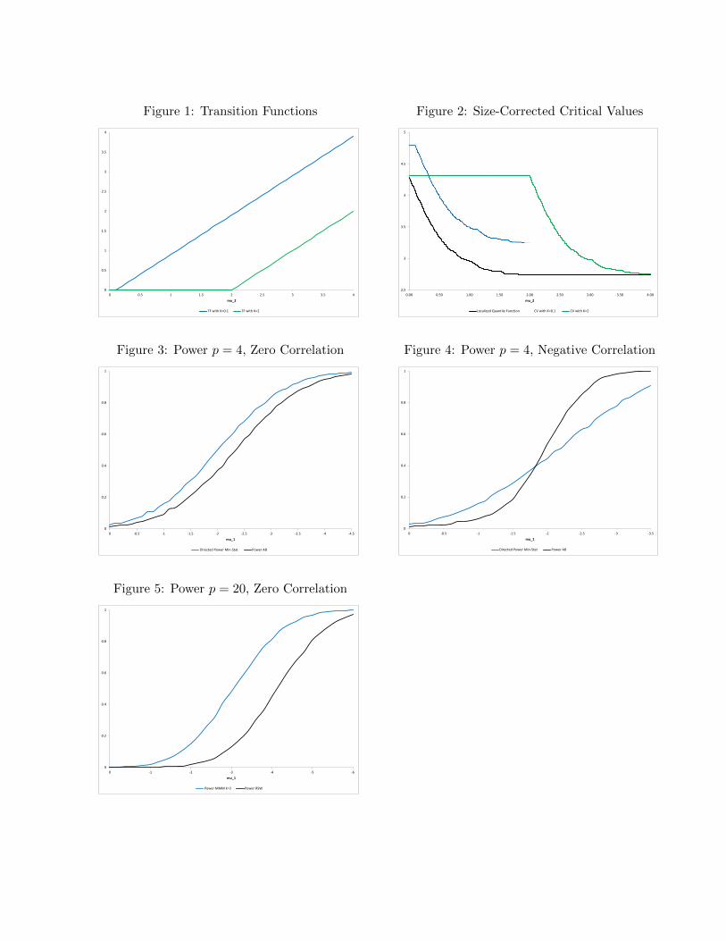
Figure 1: Transition Functions Figure 2: Size-Corrected Critical Values

0

0.5

1

1.5

2

2.5

3

3.5

4

0 0.5 1 1.5 2 2.5 3 3.5 4mu_2

TF with K=0.1 TF with K=2

2.5

3

3.5

4

4.5

5

0.00 0.50 1.00 1.50 2.00 2.50 3.00 3.50 4.00mu_2

Localized Quantile Function CV with K=0.1 CV with K=2

Figure 3: Power p = 4, Zero Correlation Figure 4: Power p = 4, Negative Correlation

0

0.2

0.4

0.6

0.8

1

0 -0.5 -1 -1.5 -2 -2.5 -3 -3.5 -4 -4.5mu_1

Directed Power Min-Stat Power AB

0

0.2

0.4

0.6

0.8

1

0 -0.5 -1 -1.5 -2 -2.5 -3 -3.5mu_1

Directed Power Min-Stat Power AB

Figure 5: Power p = 20, Zero Correlation

0

0.2

0.4

0.6

0.8

1

0 -1 -2 -3 -4 -5 -6mu_1

Power MMM k=2 Power RSW