On the control of a muscular force model

AURORE MAILLARDLe2i CNRS UMR 6306

Universite de BourgogneFranche-Comte, Arts et Metiers9 av. Alain Savary, 21000 Dijon

FRANCEaurore.maillard@u-bourgogne.fr

TOUFIK BAKIRLe2i CNRS UMR 6306

Universite de BourgogneFranche-Comte, Arts et Metiers9 av. Alain Savary, 21000 Dijon

FRANCEtoufik.bakir@u-bourgogne.fr

STEPHANE BINCZAKLe2i CNRS UMR 6306

Universite de BourgogneFranche-Comte, Arts et Metiers9 av. Alain Savary, 21000 Dijon

FRANCEstbinc@u-bourgogne.fr

Abstract: Athletes and Physiotherapists may need electromyostimulation to reinforce muscle or to treat deficientmuscles in order to speed up their recovery. Generally, the electromyostimulator does not take into account thephysiological parameters necessary to adapt automatically the stimulation parameters of the system in order toreach a desired force value. To remedy at this problem and to optimize the rehabilitation sessions, we investigatethe feasibility of controlling the muscular force by using an experimentally-based model.

Key–Words: Electrostimulation, Force muscular, Control

1 Introduction

Electromyostimulation is a process which arouses alot of interest. As a consequence, this technique isoften used for reinforcement and for reconditioning.Electromyostimulation (EMS) is carried out by plac-ing electrodes on the area to be stimulated and electri-cal pulses are sent into the muscle to create involun-tary contractions. The effects of these stimulations onthe generated force are difficult to model. The model-ing should be realized by mathematical models whichtake into account the physiological parameters, vary-ing according to the subject state but also from oneperson to another, which renders the modeling diffi-cult as explained in [1].

The model used in [2, 3] is obtained from exper-imental data and therefore satisfies specification re-quirements. Furthermore, it is based on a specific pro-tocol which proves its reliability to solve the modelingproblem of the relationship between force and stimu-lation accurately. Thus, this model could be used tomaximize the force, which could be realized for in-stance by the prediction of the necessary number ofmuscular contractions. The predicted contraction fre-quency could also be used to analyze the correlationbetween the physiological aspects and the mathemat-ical model [4]. The relationship between the forceand the stimulation frequency can also be estimatedon the same model, showing a correlation betweenthe stimulation frequency and the effects on the force[5,6]. This model was tested in the case of childrenwith cerebral paralysis (CP) in order to predict theobtained force level [7]. In this study, we based our

work on the model proposed in [2, 3], where the con-trol variable acts on the impulse amplitude while thefrequency is fixed. Section 2 details the equations ofthe model. Then in section 3, the nonlinear controlstrategy is proposed. In section 4, simulation resultsare presented, leading to quantify the control methodefficiency. Finally, section 5 is devoted to the conclu-sion.

2 ModelThe model used is defined by a set of differential equa-tions, as follows:

dCndt

=1

τc

n∑i=1

Rie−(t−ti)τc − Cn

τc, (1)

dF

dt= A

CnKm + Cn

− F

τ1 + τ2(Cn

Km+Cn), (2)

withRi = 1 + (R0 − 1)e−(

ti−ti−1τc

). (3)

Equation (1) represents the Cn derivative depend-ing on Cn the normalized amount of C2+

a − troponincomplex obtained at each stimulation, the time con-stant τc and the sum of successive pulses that are gath-ered in the term:

n∑i=1

Rie−(t−ti)τc , (4)

where ti is the time of ith pulse and Ri the mathe-matical term defining the magnitude of enhancement

Aurore Maillard et al.International Journal of Biology and Biomedicine

http://www.iaras.org/iaras/journals/ijbb

ISSN: 2367-9085 78 Volume 1, 2016

0 0.2 0.4 0.6 0.8 10

100

200

300

400

500

600700

Time (s)

For

ce (

N)

Fref= 100Fref= 200Fref= 400

Figure 1: Evolution of the force value of control forFref= 100, 200 and 400 N with dt= 10 ms.

in Cn from the next stimuli. Ri is initialized at R0.The stimulation generates a muscular force F accord-ing to (2). The parameters A (the scaling factor of theforce and the muscle shortening velocity), R0 and τ1(a force time constant) are for this model at their rest-ing values: A= 5.1 N/ms, R0=2 and τ1= 43.8 ms andthe parameters τ2= 124.4 ms,Km= 0.3 and τc= 20 ms,as defined in [2] with τ2 the second force time constantand Km the sensitivity of a strong bound crossbridgesto Cn.

3 Control MethodThe control method presented in this section is a non-linear control applied to the force model. The variableu represents the control acting on the variation of im-pulse amplitudes. These amplitudes are found in thesum of exponential functions between two successivestimulations dti = ti+1− ti. The control is defined bythe expression:

u =1

τc

n∑i=1

αiRie−(t−ti)τc , (5)

so that (1) is modified as:

dCndt

= u− Cnτc. (6)

Equation (5) includes a new parameter αi which is de-termined by the control u. Therefore, controlling theforce corresponds to finding αi values. The controlmethod is based on the prediction of the amplitudeof the next pulse with dti constant. In the first part,we consider the case of a continuous control, nameduNL(t) then we deduct from it the discrete controlu(t), leading to determine αi.

0 0.2 0.4 0.6 0.8 10

0.2

0.4

0.6

0.8

Time (s)

α

Fref= 100Fref= 200Fref= 400

Figure 2: Evolution of the obtained impulse amplitudeof control of the force for Fref= 100, 200 and 400 Nwith dt= 10 ms.

In a general way, a nonlinear affine system func-tion of uNL(t) is described by the system (7), that is:

x(t) = f(x(t)) + g(x(t))uNL(t), (7)

andy(t) = h(x(t)). (8)

According to the force model, one can write:

x(t) =

[Cn(t)F (t)

]=

[x1(t)x2(t)

], (9)

y(t) = x2(t), (10)

where f and g represent vector fields:

f =

−x1τc

Ax1x1 +Km

− x2τ1 + τ2

x1x1+Km

=

[f1f2

], (11)

gT =[1 0]T. (12)

Equation (10) expresses the fact that only theforce F (t) is measured. Let us assume that the systemis controllable, so that a control by output feedbackwould be possible. To perform this, we compute thefirst derivative of y(t). From (7) and (8), it comes:

y(t) = Lfh(x) + Lgh(x)uNL(t), (13)

whereLfh(x) =

∂h

∂xf, (14)

Lgh(x) =∂h

∂xg. (15)

It leads to:

Lfh(x) = [0 1]f = f2, (16)

Aurore Maillard et al.International Journal of Biology and Biomedicine

http://www.iaras.org/iaras/journals/ijbb

ISSN: 2367-9085 79 Volume 1, 2016

0 2 4 6 8 100

400600

1 000F

orce

(N

)

0 0.02 0.04 0.06 0.08 0.1 0.120

200

400

Time (s)

For

ce (

N)

Fref= 600

Fref= 800

Figure 3: Representation of the generated forces forthe control of the force for Fref= 600 and 800 N withdt= 10 ms.

0 0.02 0.04 0.06 0.08 0.10

2

4

6

8x 10

110

Time (s)

α

0 2 4 6 8 100

5

10x 10

111

α

Fref= 800

Fref= 600

0.0106 0.0106

1.53

1.532

1.534

Time (s)

α

Zoom

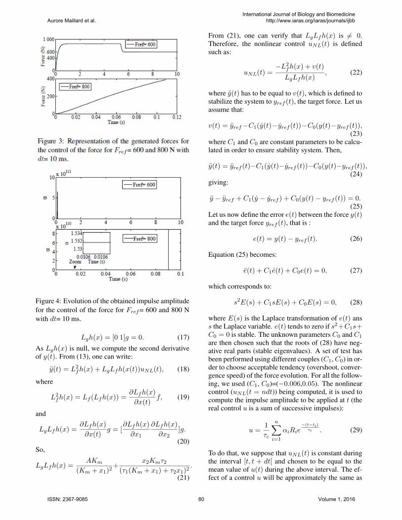
Figure 4: Evolution of the obtained impulse amplitudefor the control of the force for Fref= 600 and 800 Nwith dt= 10 ms.

Lgh(x) = [0 1]g = 0. (17)

As Lgh(x) is null, we compute the second derivativeof y(t). From (13), one can write:

y(t) = L2fh(x) + LgLfh(x(t))uNL(t), (18)

where

L2fh(x) = Lf (Lfh(x)) =

∂Lfh(x)

∂x(t)f, (19)

and

LgLfh(x) =∂Lfh(x)

∂x(t)g = [

∂Lfh(x)

∂x1

∂Lfh(x)

∂x2]g.

(20)So,

LgLfh(x) =AKm

(Km + x1)2+

x2Kmτ2(τ1(Km + x1) + τ2x1)2

.

(21)

From (21), one can verify that LgLfh(x) is 6= 0.Therefore, the nonlinear control uNL(t) is definedsuch as:

uNL(t) =−L2

fh(x) + v(t)

LgLfh(x), (22)

where y(t) has to be equal to v(t), which is defined tostabilize the system to yref (t), the target force. Let usassume that:

v(t) = yref−C1(y(t)−yref (t))−C0(y(t)−yref (t)),(23)

where C1 and C0 are constant parameters to be calcu-lated in order to ensure stability system. Then,

y(t) = yref (t)−C1(y(t)−yref (t))−C0(y(t)−yref (t)),(24)

giving:

y − yref + C1(y − yref ) + C0(y(t)− yref (t)) = 0.(25)

Let us now define the error e(t) between the force y(t)and the target force yref (t), that is :

e(t) = y(t)− yref (t). (26)

Equation (25) becomes:

e(t) + C1e(t) + C0e(t) = 0, (27)

which corresponds to:

s2E(s) + C1sE(s) + C0E(s) = 0, (28)

where E(s) is the Laplace transformation of e(t) anss the Laplace variable. e(t) tends to zero if s2+C1s+C0 = 0 is stable. The unknown parameters C0 and C1

are then chosen such that the roots of (28) have neg-ative real parts (stable eigenvalues). A set of test hasbeen performed using different couples (C1,C0) in or-der to choose acceptable tendency (overshoot, conver-gence speed) of the force evolution. For all the follow-ing, we used (C1, C0)=(−0.006,0.05). The nonlinearcontrol (uNL(t = ndt)) being computed, it is used tocompute the impulse amplitude to be applied at t (thereal control u is a sum of successive impulses):

u =1

τc

n∑i=1

αiRie−(t−ti)τc . (29)

To do that, we suppose that uNL(t) is constant duringthe interval [t, t + dt[ and chosen to be equal to themean value of u(t) during the above interval. The ef-fect of a control u will be approximately the same as

Aurore Maillard et al.International Journal of Biology and Biomedicine

http://www.iaras.org/iaras/journals/ijbb

ISSN: 2367-9085 80 Volume 1, 2016

0 1 2 3 4 50

200

400

600

800

Time (s)

For

ce (

N)

α<=0.5

α<=1

α<=2

Fref = 800 Ndt = 10 ms

Figure 5: Different limits of impulse amplitudes for aFref of 800 N (dt= 10 ms).

uNL(t) which leads F to Fref ,

uNL(t) =1

H + 1

H∑k=0

u(t+k

Hdt)

=1

H + 1

H∑k=0

1

τc

n∑i=1

Riαie

−(t+ kH dt− ti)τc ,

(30)where H is the number of simulation values of u dur-ing [t, t+dt[ equal to a choosen value fixed to 10 withthe integration step ∆T = dt

H+1 . Therefore:

uNL(t) =1

H + 1[H∑k=0

1

τc[n−1∑i=1

Riαie−(t+ k

Hdt−ti)

τc +

Rnαne−(t+ k

Hdt−tn)

τc ]], (31)

αi (i = 1, ..., n− 1) being the previous pulses ampli-tudes, which were computed using the previous stim-ulation steps. At time t = ndt, only the value of αn isunknown. From (31), it comes:

αn =

(H + 1)uNL(t)−H∑k=0

1τc

[n−1∑i=1

Riαie−(t+ k

Hdt−ti)

τc ]

Rnτc

H∑k=0

e

−(t+ kH dt− tn)

τc

.

(32)Until this step, α is considered as a free parameter.

However, it is obvious that the muscle will not bestimulated by whatever amplitude. In our case, wesuppose that αi can range between 0 and 2, whichcorresponds to 2 times the stimulation constraint im-posed in [2] (the pulse amplitude is still in an accept-able range).

4 Simulations ResultsDifferential equations of the force model (1) to (3) aresolved by numerical methods. The control method isapplied on the force model for the force referencesFref= 100, 200, 400, 600 and 800 N with stimulationtimes dt= 10, 20, 40, 60, 80, 100 ms.

In the Figures 1 and 3, the generated force forFref=100, 200, 400, 600 and 800 N is representedwith the corresponding computed α (Figures 2 and 4)(case of unconstrained α). The developed force stay-ing constant at its final value during the simulation,we represent just the obtained force for a 1 s and 10s duration. Contrary to the cases of small referencevalues (100, 200 and 400 N) where the impulse am-plitude is at most equal to 0.2 (Figure 2), the α valuesfor Fref= 600 and 800 N reach very high values (Fig-ure 4). As discussed above, the applied pulse to themuscle must have a reasonable amplitude. The effectsof this constraint is showed in Figure 5 where α islimited to 0.5, 1 and 2 for Fref= 800 N. It can be ob-served that α’s limit influences the final value of F . Infact, the smaller α is, the farther the final value of Fis from Fref .

In Figure 6, we treat the effect of dt (dt varies for10, 20, 40, 60, 80 and 100 ms) on the final value ofthe force for Fref= 100, 200, 400, 600 and 800 N. It isclear that the difference between F and Fref increaseswith dt.

To get closer to experimental results, a whitenoise of 5% seems adequate to mimic realistic con-ditions, that’s why a 5% noise is added to the forcemeasurements in all the control simulations. On theFigure 7, the obtained force is presented. At high ref-erence force, the noise is not negligible and we musttake into account the disturbance on the force and onthe stimulation. With a low reference force, the devel-oped force is not disturbed by noise.

5 ConclusionIn this work, we applied a control method to controlthe force value of a muscle during a stimulation ses-sion. The computed control method acts on the elec-trical impulse amplitude during an EMS. The simu-lation results showed a good efficiency of this con-trol by maintaining the force at the reference force.Stimulation time and impulse amplitude effects werealso explored for different cases of reference forces.A small stimulation time with a constrained impulseamplitude seems to be the best strategy to compute anefficient control. In a next study, it would be inter-esting to include muscular fatigue effects in order tocheck if this control could be still efficient then to testexperimentally.

Aurore Maillard et al.International Journal of Biology and Biomedicine

http://www.iaras.org/iaras/journals/ijbb

ISSN: 2367-9085 81 Volume 1, 2016

0 200 400 600 8000

200

400

600

800

1000

Fref (N)

For

ce (

N)

dt= 10msdt= 20msdt= 40msdt= 60msdt= 80msdt= 100msF=Fref

Figure 6: Application of the nonlinear control for thereference forces Fref= 100, 200, 400, 600 and 800 N,the obtained forces for dt= 10, 20, 40, 60, 80, 100 ms.

0 200 400 600 8000

200

400

600

800

1000

Fref (N)

For

ce (

N)

dt= 10msdt= 20msdt= 40msdt= 60msdt= 80msdt= 100msF=Fref

Figure 7: Application of the white noise of 5% for theFref= 100, 200, 400, 600 and 800 N and dt= 10, 20,40, 60, 80, 100 ms.

Acknowledgements: The authors would like tothank the Conseil Regional de Bourgogne which sup-ports the project through a young researcher contrac-tor funding

References:

[1] Z. Li, M. Hayashibe, C. Fattal and D. Guiraud,”Muscle fatigue tracking with evoked EMG viarecurrent neural network: toward personalizedneuroprosthetics”, IEEE Computational Intelli-gence Magazine, 2014, 9 (2), 38-46.

[2] J. Ding, A. S. Wexler and S. A. Binder-Macleod,”A predictive fatigue model-I: Predicting the ef-fect of stimulation frequency and pattern on fa-tigue”, IEEE Transactions on Neural Systemsand Rehabilitation, vol 10, no 1 March 2002.

[3] J. Ding, A. S. Wexler, and S. A. Binder-Macleod,”A predictive fatigue model-II: Predicting the ef-

fect of resting times on fatigue”, IEEE Transac-tions on Neural Systems and Rehabilitation, vol10, no 1 March 2002.

[4] Li-Wei Chou, Jun Ding, Anthony S. Wexler,Stuart A. Binder-Macleod, ”Predicting optimalelectrical stimulation for repetitive human mus-cle activation”, International Congress Series 15(2005) 300-309.

[5] Jun Ding, Stuart A. Binder-Macleod, AnthonyS. Wexler, ”Two-step, predictive, isometric forcemodel tested on data from human and rat mus-cles”, Journal of Applied Physiology 85 (1998)2176-2189.

[6] Jun Ding, Anthony S. Wexler, Stuart A. Binder-Macleod, ”A mathematical model that predictsthe force-frequency relationship of human skele-tal muscle”, Wiley Periodicals, Inc. MuscleNerve 26 (2002) 477-485.

[7] Samuel C. K. Lee, Jun Ding, Laura A. Prosser,Anthony S. Wexler, Stuart A. Binder-Macleod,”A predictive mathematical model of muscleforces for children with cerebral palsy”, Devel-opmental Medicine and Child Neurology, 2009,51: 949-958.

Aurore Maillard et al.International Journal of Biology and Biomedicine

http://www.iaras.org/iaras/journals/ijbb

ISSN: 2367-9085 82 Volume 1, 2016