Working Paper 04-40

Economics Series 15 July 2004

Departamento de Economía

Universidad Carlos III de Madrid Calle Madrid, 126

28903 Getafe (Spain)

Fax (34) 91 624 98 75

ON THE DEFINITION OF AFFORDABLE PRICES UNDER UNIVERSAL SERVICE OBLIGATIONS *

Ramiro Losada1

Abstract In this paper, we investigate the social welfare implications of the European and American

definition of affordable prices when a country is divided into independent zones. We find that the

European definition is always soc ial welfare superior, because it forces to keep lower prices. We

also introduce to new defintions of affordable prices. The first definition advocates for a common

price for the unprofitable area. We prove that this definition is social welfare superior to the

current definitions. In the second definition denote as “yardstick pricing” , we define the

affordable prices for the unprofitable areas as a function that does not depende on their own zone

profitable area price. We show that yardstick price is more efficient for social welfare when the

differences in demand among zones are not very large .

* I gratefully acknowledge the research supervision of M. Angeles de Frutos and Pedro L. Marín. I also thank the Spanish Ministry of Education and Culture for financial support, grant AP2000-0847. The usual disclaimer applies.

1 Department of Economics, Universidad Carlos III de Madrid, Calle Madrid 126, 28903, Getafe, Spain, Tlf: +34 91 6249367, Fax: +34916249875, Email: losada @eco.uc3m.es.

Working Paper 04-33 Economics Series 12 July 2004

Departamento de Economía Universidad Carlos III de Madrid

Calle Madrid, 126 28903 Getafe (Spain)

Fax (34) 91 624 98 75

ON THE DEFINITION OF AFFORDABLE PRICES UNDER UNIVERSAL SERVICE OBLIGATIONS *

Ramiro Losada1

Abstract In this paper, we investigate the social welfare implications of the European and American

definition of affordable prices when a country is divided into independent zones. We find that the

European definition is always social welfare superior, because it forces to keep lower prices. We

also introduce to new definitions of affordable prices. The first definition advocates for a common

price for the unprofitable area. We prove that this definition is social welfare superior to the

current definitions. In the second definition denote as “yardstick pricing” , we define the

affordable prices for the unprofitable areas as a function that does not depend on their own zone

profitable area price. We show that yardstick price is more efficient for social welfare when the

differences in demand among zones are not very large.

* I gratefully acknowledge the research supervision of M. Angeles de Frutos and Pedro L. Marín. I also thank the Spanish Ministry of Education and Culture for financial support, grant AP2000-0847. The usual disclaimer applies.

1 Department of Economics, Universidad Carlos III de Madrid, Calle Madrid 126, 28903, Getafe, Spain, Tlf: +34 91 6249367, Fax: +34916249875, Email: losada @eco.uc3m.es.

On the Definition of Affordable Prices underUniversal Service Obligations ∗

Ramiro Losada†

May 2004

Abstract

In this paper, we investigate the social welfare implications of theEuropean and American definition of affordable prices when a countryis divided into independent zones. We find that the European defini-tion is always social welfare superior, because it forces to keep lowerprices. We also introduce two new definitions of affordable prices. Thefirst definition advocates for a common price for the unprofitable area.We prove that this definition is social welfare superior to the currentdefinitions. In the second definition denoted as ”yardstick pricing”,we define the affordable prices for the unprofitable areas as a functionthat does not depend on their own zone profitable area price. Weshow that yardstick pricing is more efficient for social welfare whenthe differences in demand among zones are not very large.

Keywords : Universal Service Obligations, Affordable Price, So-cial Welfare.

JEL Classification : I31,L96.

∗I gratefully acknowledge the research supervision of M. Angeles de Frutos and Pedro L.Marin. I also thank the Spanish Ministry of Education and Culture for financial support,grant AP2000-0847. The usual disclaimer applies.

†Dpto de Economia. Universidad Carlos III de Madrid. c/ Madrid no126, 28903,Getafe, Spain. Tlf: +34916249367. Fax: +34916249875 E-mail: losada@eco.uc3m.es

1

1 Introduction

In the telecommunications market regulators place a high value to the ac-cess of all consumers to the service. This goal has been termed UniversalService. There are several reasons why regulators may want to pursue thegoal of universal service, such as equity, economic development, and even eco-nomic efficiency (due to sizeable network externalities). One of the importantcharacteristic of the telecommunications markets is that some countries, e.g.USA or Argentina, have divided their national territory in independent zones,where each zone is a market on its own.1

Universal Service has been defined by European and American authori-ties in a similar way. The European Parliament and the Council stipulate theobligation for the member states that Universal Service is a set of services”made available with the quality specified to all end-users in their territory,irrespective of their geographical location, and, in the light of specific nationalconditions, at an affordable price”.2 The American regulator concept of Uni-versal Service consists in ”ensuring quality telecommunications services ataffordable rates to consumers, in all regions of the nation, including rural,insular, and high-cost areas”.3 Thus one of the most important UniversalService goals is that all consumers must enjoy affordable prices.4

Although both regulations seek to set affordable prices, what the differ-ent regulators understand for affordable prices is not exactly the same. Ifwe take the American definition of affordable prices, we find: ”the Commis-sion shall adopt rules to require that the rates charged by providers of in-terexchange telecommunication services to subscribers in rural and high costmarkets shall not be higher than the rates charged by each such provider toits suscriber in urban markets. Such rules shall also require that a providerof interstate interchange telecommunications services shall provide such ser-vices to its subscribers in each state at rates no higher than the rates chargedto its subscribers in any other state”.5 Applying this definition, we find that,

1There is a tendency to split up the national telecommunication markets, for examplein Australia, the government has recently announced that it will introduce competitioninto USO provision by inviting carriers to tender for the USO in two regional pilot areas.

2For further details, see the Directive 2002/22/CE of the European Parliament and theCouncil.

3For further details, see Federal Communications Commission (1996), Docket n 96-45.4This requirement of the Universal Service arises because the price differentials expected

to prevail in an unregulated setting are deemed unacceptable by regulators.5For further details, see Telecommunications act (1996)

2

within USA, there may be different prices.On the other hand, if we check the European definition of affordable

prices, we find: ”Affordable price means a price defined by Member Statesat National level in the light of specific national conditions, and may involvesetting common tariffs irrespective of location or special tariff options to dealwith the needs of low-income users. Affordability for individual consumersis related to their ability to monitor and control their expenditure”.6 Thus,the European Union opts for setting a unique price per country, what inprinciple is more restrictive. Although within EU there can be countrieswith the national market divided in independent zones where firms do notoperate simultaneously in all zones, all firms are obliged to set the same price.We have that there are two streams about how to set affordable prices, onemore restrictive, the European, and the other, the American, more concernedwith the ”no intervention” paradigm.

In order to attain the objectives of Universal Service, the regulator mustimpose Universal Service Obligations (USOs hereafter) on the industry.7 Inthe case of affordable prices, USOs are constraints imposed by regulatorson firms. These constraints take the form of either uniform pricing, whichforces the firms to offer their services to all its consumers at a geographicallyuniform price, or a price cap, which establishes a maximum average priceof firms’ services. Telecommunications markets are generally characterizedby a small number of networks, so that the resulting competition will beoligopolistic. This makes that constraints imposed by USOs may createstrategic effects, and therefore affect competition.

The academic literature has not treated very deeply the definition of af-fordable prices. Few papers, Valletti et al. (2002) or Iozzi (2001), study theimpact of the price constraints on competition. They compare the scenariowhere there is a unique zone which consists in two markets (profitable andunprofitable) with no price restrictions with a scenario where firms are forcedto set a uniform price in both markets. In these papers, as in others suchas Chone et al. (2002), Anton et al. (2002), Gasmi et al. (2000) or Rosstonand Wimmer (2000), the key point is that they consider only an unprof-itable market and a profitable market. In this context, they always consider

6For further details, see Directive 2002/22/CE of the European Parliament and Council(2002).

7In the countries where the Telecommunication market was recently open to competi-tion, for example Spain, USOs are only applied to the Incumbent Carrier, Telefonica inthe case of Spain.

3

that an affordable price for the unprofitable market is equal to the price ofthe profitable market.8 With this common setup, the literature concludesthat setting a common price in both, the unprofitable and profitable mar-ket, creates an strategic link between both markets that makes higher theequilibrium price. This is so, because one of the firms is a monopolist in theunprofitable market. This firm is always interesting in relaxing competitionin the profitable market to enjoy a higher profit in the unprofitable marketthrough a price increase.

In this paper, we address the question of which of the regulatory defini-tions of affordable prices at work is better from a social point of view. Thisneeds of models which are closer to reality. We need to extend the existingmodels of USOs by considering a country which is divided in zones where eachzone consists in an unprofitable area and a profitable area.9 We also proposetwo new definitions of affordable prices. In one of these definitions, the pricein all unprofitable areas in the country is a convex combination of the pricesin the profitable areas. In the other definition, we propose that the price inany unprofitable area is a function, e.g. the sample mean, of the prices of allprofitable areas but the profitable area the unprofitable area is attached to.We denote this definition of affordable prices ”yardstick pricing”.

To do so, we extend the model by Anton et al. (2002). We need toconsider that the country is divided in more than one independent zone, eachone with one profitable area and one unprofitable area.10 We show that theEuropean regulation is social welfare superior to the American regulation.11

This is because the European regulation applies to the whole country theminimum price between the different prices that the American regulationsets in the different zones of the country.

We also show that our first definition of affordable prices is welfare supe-rior to the European. Setting the same price in all the unprofitable areas asa convex combination of the prices in the profitable areas allows us to break

8In some of these papers, it is defined the price of the unprofitable area as lower orequal than the price in the profitable area. In equilibrium, both prices are always equal.

9All the unprofitable areas form the profitable market. All the profitable areas formthe profitable market.

10We represent our set-up with a graph in Figure 1. Area 1 of the U market and area 1of the R market form zone 1. Area 2 of the U market and area 2 of the R market form zone2. This is the present situation in Argentina and USA, where the countries are divided inmore than one independent zone.

11Under the assumption taken by the literature of only one zone (which consists in thewhole unprofitable area and the whole profitable area), both regulations are identical.

4

partially the strategic link between the profitable and unprofitable areas. Wecan enjoy scenarios where the social welfare is at least equal to the situationwhere the country enjoys the price from the European regulation for some ofthe areas but for one profitable area which enjoys an even lower price.

To conclude we show that with our second definition, yardstick pricing,we can break completely the strategic link between the profitable and unprof-itable areas. This leads to a much lower price than under current regulatoryregimes definitions and the first proposed definition. But there is a limit tothis definition. We need consumers’ demands in the different zones to bevery similar. Otherwise, it may yield undesirable social welfare results.

This paper is organized as follows. Section 2 describes the model. Section3 analyzes the current regulatory frameworks and their implications for SocialWelfare. In Section 4, the first new definition of affordable prices is presentedand analyzed. In section 5, we present and analyze yardstick pricing. Section6 concludes.

2 The model

2.1 Costs and Demands

A country has two differentiated markets, one urban (U) and one rural (R).Demand in the U market is DU(p) = 1− p, and in the R market is DR(p) =b(1− p), where p is the market price and b > 0. Both market demands havea common price intercept at p = 1, whereas the slope coefficient b allows theR market demand to be smaller or larger than the U market demand. Inmany situations, we expect the R market demand to be smaller.12

Each market is divided into two areas that can be of equal or differentsize. We denote by DU

1 (p) = α1(1− p) and DU2 (p) = α2(1− p) , α1 + α2 = 1,

the demands of areas 1 and 2 of the U market. The demands of areas 1 and 2of the R market are, respectively, DR

1 (p) = β1b(1−p) and DR2 (p) = β2b(1−p),

with β1 + β2 = 1. Each area of the R market is attached to one of the areasof the U market, to constitute a zone. More precisely, area 1 of the R marketis attached to area 1 of the U market, and area 2 of the R market is attached

12This modelling strategy for the demand functions is taken from Anton et al (2002).Note that they describe a country where the differences between consumers in the twomarkets are not large.

5

to area 2 of the U market.13 They constitute zone 1 and zone 2 respectively.To further clarify the country division, see figure 1.

The fixed cost of area 1 and 2 of the U market are respectively FU1 and

FU2 . The fixed costs of area 1 and 2 of the R market are FR

1 and FR2 .14 There

is a constant marginal cost, c, which is the same for the whole country. Weassume, without loss of generality, that c = 0.15 Finally, there is a duopoly ineach zone. To simplify the analysis, we assume that no firm operates in bothzones. The firms that serve the areas of the R market and the subsidies thatthese firms receive for being in charge of USOs are determined by a politicaldecision, and it is here exogenously given.

2.2 The game

We consider a simple complete information game. The timing of the gamegoes as follows:

1. Firms in both duopolies choose quantities in their areas of the U market.We denote by qij, the quantity that the firm i = S, N produces in thearea j = 1, 2, where S denotes the firms which provides the serviceobligations and hence operates in both areas, and N denotes the firmwhich only operates in the U area. The prices in each area of the Umarket are:

pUj = 1− (qSj + qNj)

αj

, j = 1, 2

2. The prices in the areas of the R market are determined through differentrules which depend on the definition of affordable prices the governmentadopts.

3. Each firm payoffs are realized, where firms payoffs are the sum of theprofits, including any subsidy.

13This set-up is consistent, for instance, with the situation in Argentina and the USA.Both countries have been divided into zones, and within zones there are profitable andunprofitable areas.

14In general, we may suppose that the size of the fixed costs are not perfectly correlatedwith the size of the demand that each area has. Under this assumption, we can model allkind of countries, with different density of population and orography.

15This assumption is consistent with the fact that variable costs in industries that sup-port USOs are close to zero, as for example in telecommunications or water.

6

The Cournot competition in the U market serves to streamline the anal-ysis and allow us to consider a homogeneous good for which the cross-areaprice constraints are unambiguous.16 We look for the subgame perfect equi-librium of this game focusing on pure strategies.

2.3 Social Welfare

We take two different measueres of social welfare. In the first one, SW1, socialwelfare is the sum of consumers surplus plus firms profits in each zone. This isthe standard definition of social welfare when analyzing regulatory problems.In the second one, SW2, social welfare is only the sum of consumers’ surplusin the R market.17 This is an extreme representation of using USOs as a wayto promote a more harmonious distribution away from large metropolitanareas.18

3 Benchmarks: Current definitions of afford-

able prices

We begin our discussion by studying the different definitions of affordableprices and their implications for social welfare.

As we have described in the introduction, we face two different streamson how to set affordable prices when a country has more than one profitableand unprofitable area. We study first the one leaded by the Federal Com-munication Commission in the USA. This definition advocates for a pricecap in each area of the R market in such a way that the price cannot belarger than the price set in the area of the U market which it is attached to,i.e. pR

j ≤ pUj , for j = 1, 2.19 In other words, within a zone, consumers in the

R area cannot be charged higher prices than consumers in the U area. We

16As an alternative strategic mode, we could employ price setting competition (differen-tiated Bertrand). While this does not alter the basic strategic link between the U and Rmarkets, it does introduce additional issues such as how to interpret the cross-areas priceconstraints when products are differentiated.

17SW2 is consistent with a regulator who wants to base distributional comparisons onthe well-being of the USOs target group.

18Alternatively, it can be argued that SW2 represents the objective function of a reg-ulator captured by rural consumers. In a different context than ours, it has been shownthat the strong farmer unions may capture a regulator by political lobbying.

19For further details, see Telecommunications Act (1996), section 254.

7

introduce this constraint into our game at the third stage, and we proceedto solve it by backward induction. 20

First, we look for the price in the areas of the R market. It is straight-forward to see that the constraints pR

j ≤ pUj are going to be binding in

equilibrium. Note that the monopoly prices in the areas of the R market arehigher than the equilibrium prices in the respective areas of the U market,so that pR

j = pUj , for both j = 1, 2.

At the second stage, we search for the equilibrium quantities. Recall thatwe denote by qij the quantity that firm i = S, N , supplies in the U area ofthe zone it belongs to. Thus, given the quantities supplied in each area of theU market, prices in zone j are pU

j = 1− (qSj+qNj)

αjfor j = 1, 2. Consequently,

using pRj = pU

j , profits for the firms that operate in both areas of a givenzone are:

ΠSj = (1− (qSj + qNj)

αj

)(qSj +βjb(qSj + qNj)

αj

)− FUj − FR

j + sj,

where sj stands for the subsidy that a firm providing USOs receives fromthe government.

Profits for the firms that only operate in the U areas are:

ΠNj = (1− (qSj + qNj)

αj

)qNj − FUj .

Given the profit functions, we derive the reaction functions, which are:

rSj(qNj) =αj

2− (αj + 2βjb)qNj

2(αj + βjb)

rNj(qSj) =αj − qSj

2.

20Given the resulting model, there are some remarks that should be made. First, theadopted time of events is the one that makes the cross-areas constraints operate in anatural way. If quantities in both markets were set simultaneously, it would create theproblem of how to impose the price constraints in the areas of the R market. Second, thefirms that provide USOs should not be viewed as price takers in the areas of the R market.Given the cross-areas price constraints, the firms are free to set any price in the areas ofthe R market up to the ceiling. More importantly, the ceiling is endogenous with respectto the firms actions.

8

The reaction functions yield the equilibrium quantities:

q∗Sj =α2

j

3αj + 2βjb, q∗Nj =

αj(αj + βjb)

3αj + 2βjb,

and the equilibrium prices under the American regulation:

pUAj =

(αj + βjb)

3αj + 2βjb, j = 1, 2.

From these equilibrium prices, we can derive two kind of conclusions.First, the prices across zones are different. Second, in each zone there is astrategic link between the U and R areas that makes the equilibrium pricesto be higher than in a standard Cournot model.21 If we take the derivativeof the price with respect to αj and βj, we see that it is negative with respectto the former and positive with respect to the latter. This shows that thestrategic link within a zone is stronger when the relative weight of the R areabecomes larger. This is so because the firm S, which operates in both areas,is more interested in relaxing competition in the U area the larger is the Rarea that it can be monopolized. The question that remains unanswered ishow should the areas be to obtain the maximum possible social welfare.

Proposition 1 A regulator must set αj = βj to maximize social welfareunder both SW1 and SW2.

The implications of proposition 1 are several. First, it establishes thatthe R market must be divided so as to replicate the division of the U market.Consequently, the size of the U market areas must be taken into account whendeciding upon the division of the R market. Second, at the optimal division,prices do not vary across geographical zone. More precisely, at αj = βj, wehave pUA

1 = pUA2 = pR

1 = pR2 .22

We turn now to analyze the implications of the European Councildefinition of affordable prices. This definition advocates for a common pricein the whole country.23 This definition is more restrictive, because it adds

21The existence of this strategic link is shown in Anton et al. (2002) and Valletti et al.(2002).

22Therefore, the set-ups analyzed in papers as Anton et al. (2002) or Valletti et al.(2002) are optimal under the American Regulation.

23For further details, see Directive 2002/22/CE of the European Parliament and theCouncil.

9

to the American definition a new constraint. This new constraint consists inforcing zone 1 to set the same price than zone 2. In principal, this opens twopossibilities, depending on whether the regulator can decide on the size of theareas of the U and R markets or not. If the regulator can decide α1 and β1

the regulation can be trivially fulfilled without affecting the firms decisions.But, if on the contrary, α1 and β1 are given, then the European regulationmay have a bite on welfare. In what follows we analyze these two cases.

Proposition 2 If α1

β1= 1, zone 1 and the zone 2 enjoy the same price than

under the American definition.

If α1=β1, the strategic link between the area 1 of the U market and area1 of the R market is as strong as the strategic link between the area 2 ofthe U market and area 2 of the R market. This gives raise to equal prices inboth zones.

The most likely situation for a regulator is that she cannot decide thesize of the areas of the U and R markets.24 In this case, if the regulator doesnot impose a new restriction on the firms, the prices in both zones would bedifferent as it was shown when analyzing the American definition.

Proposition 3 If α1

β16= 1, the regulator introduces the price-cap pUE

j ≤min{PUA

1 , PUA2 }, j = 1, 2 to ensure the same price for the whole country.

Note that pUA1 and pUA

2 are the equilibrium prices that firms would chooseif they were under the American definition of affordable prices, whereas pUE

j

is the price under the European Regulation in area 1 and 2 of the U market.The regulator needs to impose this new price-cap to ensure that the priceswithin the zones 1 and 2 are the same. One may think that other commonprices for the country are possible by using another kind of price cap as itmay be a convex combination of pU

1 and pU2 or even the maximum of both

prices. But, under either possibility, prices across zones will not be equal.There is another alternative to ensure a unique price in the whole country.

This alternative consists in the regulator setting directly the price but we donot consider it because it is too intrusive.

The remaining question that we now try to answer is which definitionbrings the highest social welfare. The ranking is unambiguous under eithermeasure of social welfare. This is the content of next proposition

24There are very little chances for a regulator of diving the country as she wishes dueto either political or physical reasons.

10

Proposition 4 The European definition brings higher social welfare than theAmerican definition.

The intuition behind Proposition 4 is straightforward. We show in Propo-sition 3 that the European definition is implemented using the prices derivedunder the American definition and adding a new price-cap. This price-capforces to lower the price in the zone where it was higher, keeping constant thelowest price. So, at the end of the day, with the European definition there isa zone where the price is the same as in the American definition, and a zonewhere the price is lower, what means that the social welfare is higher underthe European definition.

4 An alternative definition (I): a common price

for the R market

We introduce a new definition of affordable price. We propose that all con-sumers in the whole R market have to pay the same price regardless of thegeographic zone where they live. In other words, areas 1 and 2 of the Rmarket share the same price. We will model this definition by imposing aprice cap on the price in the R market, so that pR cannot be larger than theconvex combination of the prices in the U areas, that is pR ≤ θpU

1 +(1−θ)pU2 ,

θ ∈ [0, 1].25

As in the other cases, we introduce this definition into our game in thethird stage. In addition, we now need to add up a new stage prior to thefirst stage of the primitive game, where a regulator decides about the valueof θ in order to maximize social welfare.26 Once we have defined the game,we solve it using backward induction. As in the previous cases, it is alsostraightforward to see that the constraint pR ≤ θpU

1 + (1 − θ)pU2 will be

binding in equilibrium. The monopoly prices in the areas of the R marketare higher than the convex combination of the equilibrium prices in the areasof the U market. Thus pR = θpU

1 + (1− θ)pU2 .

25This definition tries to capture the regulatory police on USOs by OFTEL. In July1997, OFTEL established the level of Universal Service for the 4 year period from 1997 to2001 as comprising the provision of universal services at ”geographically averaged prices.”.

26It is worthy to point out that the equilibrium prices in the areas of the U market maybe different across zones under this definition.

11

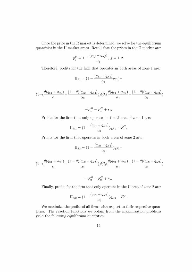
Once the price in the R market is determined, we solve for the equilibriumquantities in the U market areas. Recall that the prices in the U market are:

pUj = 1− (qSj + qNj)

αj

, j = 1, 2.

Therefore, profits for the firm that operates in both areas of zone 1 are:

ΠS1 = (1− (qS1 + qN1)

α1

qS1)+

(1−(θ(qS1 + qN1)

α1

+(1− θ)(qS2 + qN2)

α2

))bβ1(θ(qS1 + qN1)

α1

+(1− θ)(qS2 + qN2)

α2

)

−FR1 − FU

1 + s1.

Profits for the firm that only operates in the U area of zone 1 are:

ΠN1 = (1− (qS1 + qN1)

α1

)qN1 − FU1 .

Profits for the firm that operates in both areas of zone 2 are:

ΠS2 = (1− (qS2 + qN2)

α2

)qS2+

(1−(θ(qS1 + qN1)

α1

+(1− θ)(qS2 + qN2)

α2

))bβ2(θ(qS1 + qN1)

α1

+(1− θ)(qS2 + qN2)

α2

)

−FR2 − FU

2 + s2.

Finally, profits for the firm that only operates in the U area of zone 2 are:

ΠN2 = (1− (qS2 + qN2)

α2

)qN2 − FU1 .

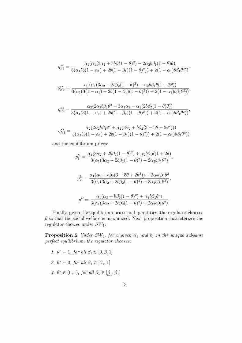
We maximize the profits of all firms with respect to their respective quan-tities. The reaction functions we obtain from the maximization problemsyield the following equilibrium quantities:

12

q∗∗S1 =α1(α1(3α2 + 3bβ(1− θ)2)− 2α2bβ1(1− θ)θ)

3(α1(3(1− α1) + 2b(1− β1)(1− θ)2)) + 2(1− α1)bβ1θ2)),

q∗∗N1 =α1(α1(3α2 + 2bβ2(1− θ)2) + α2bβ1θ(1 + 2θ))

3(α1(3(1− α1) + 2b(1− β1)(1− θ)2)) + 2(1− α1)bβ1θ2)),

q∗∗S2 =α2(2α2bβ1θ

2 + 3α1α2 − α1(2bβ2(1− θ)θ))

3(α1(3(1− α1) + 2b(1− β1)(1− θ)2)) + 2(1− α1)bβ1θ2)),

q∗∗N2 =α2(2α2bβ1θ

2 + α1(3α2 + bβ2(3− 5θ + 2θ2)))

3(α1(3(1− α1) + 2b(1− β1)(1− θ)2)) + 2(1− α1)bβ1θ2))

and the equilibrium prices:

pU1 =

α1(3α2 + 2bβ2(1− θ)2) + α2bβ1θ(1 + 2θ)

3(α1(3α2 + 2bβ2(1− θ)2) + 2α2bβ1θ2),

pU2 =

α1(α2 + bβ2(3− 5θ + 2θ2)) + 2α2bβ1θ2

3(α1(3α2 + 2bβ2(1− θ)2) + 2α2bβ1θ2),

pR =α1(α2 + bβ2(1− θ)2) + α2bβ1θ

2)

3(α1(3α2 + 2bβ2(1− θ)2) + 2α2bβ1θ2).

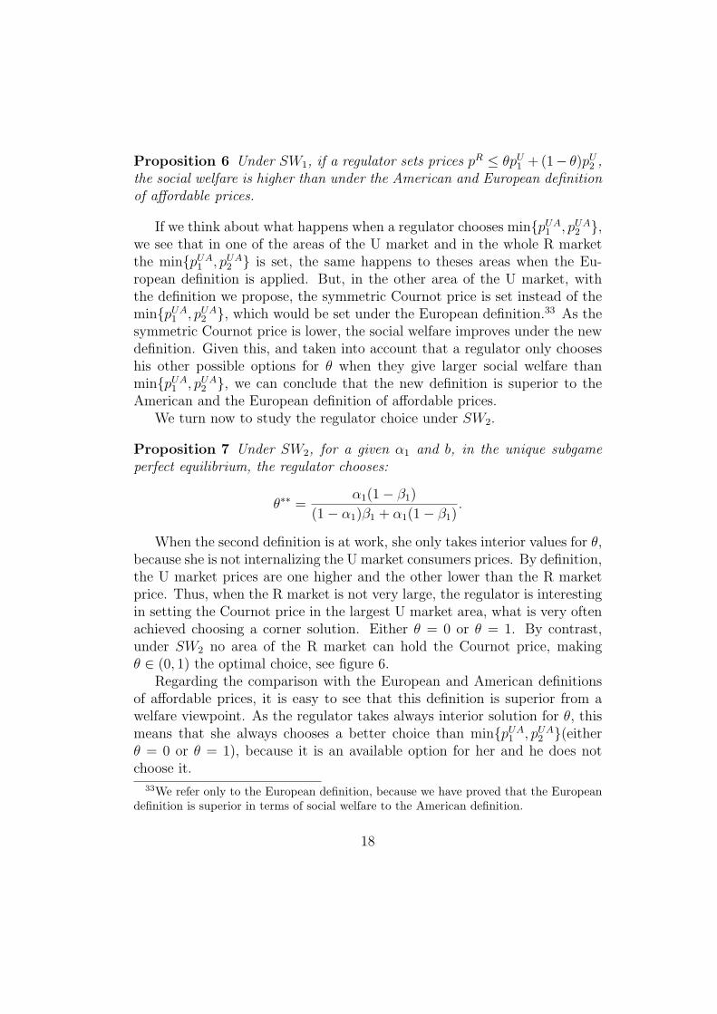
Finally, given the equilibrium prices and quantities, the regulator choosesθ so that the social welfare is maximized. Next proposition characterizes theregulator choices under SW1.

Proposition 5 Under SW1, for a given α1 and b, in the unique subgameperfect equilibrium, the regulator chooses:

1. θ∗ = 1, for all β1 ∈ [0, β11]

2. θ∗ = 0, for all β1 ∈ [β1, 1]

3. θ∗ ∈ (0, 1), for all β1 ∈ [β1, β1]

13

where β1

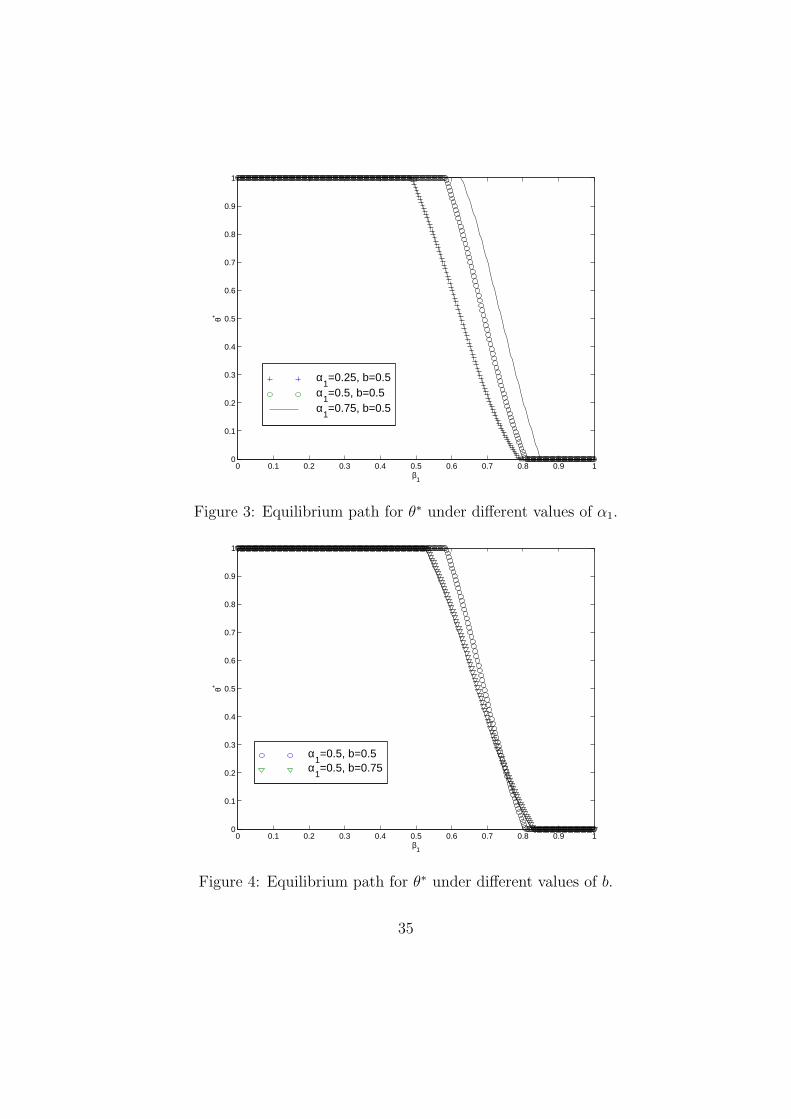
is an increasing function on α1 and b, and β1 is an increasingfunction on α1 and decreasing on b.

To analyze deeply the implications of this new definition we focus on threecases: θ∗ = 0, θ∗ = 1 and θ∗ = 1

2. We only study these three cases for two

reasons. First, because θ∗ = 0, θ∗ = 1 are the most likely equilibria. Second,we have also chosen θ∗ = 1

2as a representation of an interior equilibria

because if we consider all possible equilibria, the analysis becomes rathercomplex as to allow us to get any conclusive result.

Note that, in equilibrium, this definition of affordable prices can be easilyredefined when we consider only the equilibria θ∗ = 0 and θ∗ = 1, either aspR = min{pUA

1 , pUA2 } or as pR = max{pUA

1 , pUA2 }.27

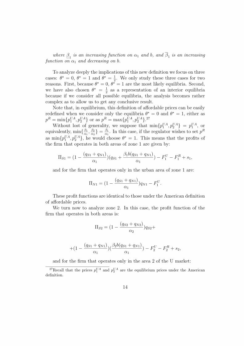
Without lost of generality, we suppose that min{pUA1 , pUA

2 } = pUA1 , or

equivalently, min{ β1

α1, β2

α2} = β1

α1. In this case, if the regulator wishes to set pR

as min{pUA1 , pUA

2 }, he would choose θ∗ = 1. This means that the profits ofthe firm that operates in both areas of zone 1 are given by:

ΠS1 = (1− (qS1 + qN1)

α1

)(qS1 +β1b(qS1 + qN1)

α1

)− FU1 − FR

1 + s1,

and for the firm that operates only in the urban area of zone 1 are:

ΠN1 = (1− (qS1 + qN1)

α1

)qN1 − FU1 .

These profit functions are identical to those under the American definitionof affordable prices.

We turn now to analyze zone 2. In this case, the profit function of thefirm that operates in both areas is:

ΠS2 = (1− (qS2 + qN2)

α2

)qS2+

+(1− (qS1 + qN1)

α1

)(β2b(qS1 + qN1)

α1

)− FU2 − FR

2 + s2,

and for the firm that operates only in the area 2 of the U market:

27Recall that the prices pUA1 and pUA

2 are the equilibrium prices under the Americandefinition.

14

ΠN2 = (1− (qS2 + qN2)

α2

)qN2 − FU2 .

If we look at the profit functions, we can see that firm S2 profit functiondepends upon quantities qS1 and qN1. Taking into account this fact, themaximization problem reduces to a symmetric Cournot problem where onlyarea 2 of the U market matters. This means that consumers in area 2 of theU market enjoy a lower price. To summarize, the R market and area 1 ofthe U market share the same price which is pUA

1 . Firms in the area 2 of theU area set the symmetric Cournot price which is lower.28

We can make a similar analysis for the case where pR = max{pUA1 , pUA

2 },so that pR = max{ β1

α1, β2

α2}. If we suppose that max{pUA

1 , pUA2 } = pUA

2 , inequilibrium, firms in the R market and in the area 1 of the U area set anequal price which is higher than the symmetric Cournot price which is set inthe area 2 of the U market.29

Now, we analyze under what conditions a regulator decides to choosepR = max{pUA

1 , pUA2 } (θ∗ = 0) instead of pR = min{pUA

1 , pUA2 } (θ∗ = 1) or the

equilibrium price that comes out from θ∗ = 12.

We analyze first when the regulator chooses pR = max{pUA1 , pUA

2 } insteadof pR = min{pUA

1 , pUA2 }. At first sight, we may think that a regulator should

always choose pR = min{pUA1 , pUA

2 }, because it ensures the minimum pricefor three out of the four areas, and in addition, the remaining area enjoys thesymmetric Cournot price. This may be a reasonable argument, but it is notalways right. For example, one can imagine an scenario where the oppositeholds. Consider a situation as the one described graphically in the figure 3of the appendix. For this case α1 < α2, and α1 < β1 < β2. In this scenariopUA

1 > pUA2 , but pUA

1 − pUA2 can be arbitrarily small. If the regulator chooses

the minimum prices then pR = pUA2 = pU

2 and pU1 = pC , if the regulator

chooses the maximum prices then pR = pUA1 = pU

1 and pU2 = pC , where pC is

the symmetric Cournot price.If the regulator chooses pUA

1 , she gets the symmetric Cournot price forthe area 2 of the U market, which is much larger than the area 1 of the Umarket. Thus, the regulator prefers to set pR = max{pUA

1 , pUA2 }, because the

loss in social welfare in the whole R market and in area 1 of the U market ismore than overcome by the price drop in the area 2 of the U market.

28Even though pU2 < pU

1 = pUA1 = pR, it is still true that pUA

2 ≥ pUA1

29Now pR = pUA2 = pU

2 ≥ pUA1 > pU

1

15

This example has shown that the optimal decision may involve to choosethe maximum price. To analyze this issue further, assume without loss ofgenerality that the area 1 of the R market is always bigger than the area 1 ofthe U market, so that α1 < β1.

30 Then, a regulator chooses max{pUA1 , pUA

2 }when the following condition holds:

α1pC + α2p

UA1 + bpUA

1 < α1pUA2 + α2p

C + bpUA2 .

This condition means that a regulator chooses max{pUA1 , pUA

2 } instead ofmin{pUA

1 , pUA2 } when the sum of the prices, weighted by the size of the areas

where they are set, is lower under max{pUA1 , pUA

2 }.31 If we operate the lattercondition, we obtain that it can be written as:

α1 + b

α2 + b<

β2(3α1 + 2β1b)

β1(3α2 + 2β2b).

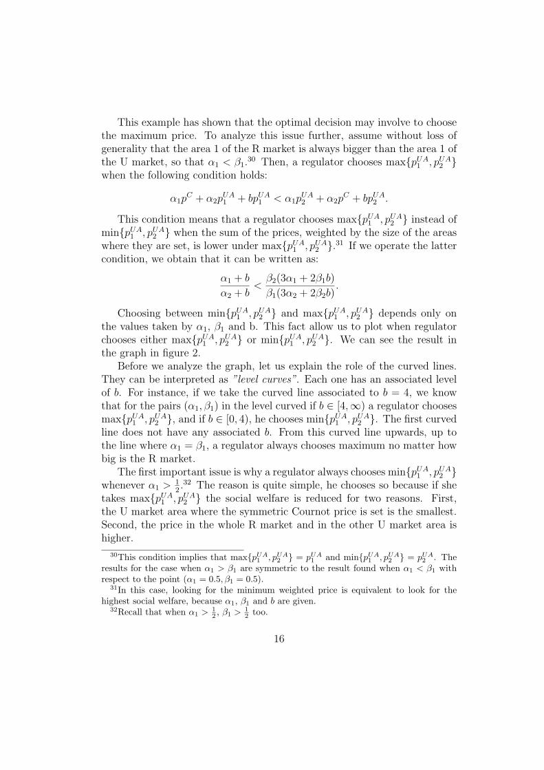
Choosing between min{pUA1 , pUA

2 } and max{pUA1 , pUA

2 } depends only onthe values taken by α1, β1 and b. This fact allow us to plot when regulatorchooses either max{pUA

1 , pUA2 } or min{pUA

1 , pUA2 }. We can see the result in

the graph in figure 2.Before we analyze the graph, let us explain the role of the curved lines.

They can be interpreted as ”level curves”. Each one has an associated levelof b. For instance, if we take the curved line associated to b = 4, we knowthat for the pairs (α1, β1) in the level curved if b ∈ [4,∞) a regulator choosesmax{pUA

1 , pUA2 }, and if b ∈ [0, 4), he chooses min{pUA

1 , pUA2 }. The first curved

line does not have any associated b. From this curved line upwards, up tothe line where α1 = β1, a regulator always chooses maximum no matter howbig is the R market.

The first important issue is why a regulator always chooses min{pUA1 , pUA

2 }whenever α1 > 1

2.32 The reason is quite simple, he chooses so because if she

takes max{pUA1 , pUA

2 } the social welfare is reduced for two reasons. First,the U market area where the symmetric Cournot price is set is the smallest.Second, the price in the whole R market and in the other U market area ishigher.

30This condition implies that max{pUA1 , pUA

2 } = pUA1 and min{pUA

1 , pUA2 } = pUA

2 . Theresults for the case when α1 > β1 are symmetric to the result found when α1 < β1 withrespect to the point (α1 = 0.5, β1 = 0.5).

31In this case, looking for the minimum weighted price is equivalent to look for thehighest social welfare, because α1, β1 and b are given.

32Recall that when α1 > 12 , β1 > 1

2 too.

16

On the other hand, we find a region where a regulator always sets a priceequal to max{pUA

1 , pUA2 }. This region starts in the line where α1 = β1, and

continues downwards until the first curved line is reached. If we take theextreme case, α1 → β1, we easily see that the social welfare is always higherwhen the regulator takes max{pUA

1 , pUA2 }. The symmetric Cournot price is

in the largest U market area, while the increase in the price of the otherthree areas is negligible. The same occurs in the whole region, althoughthe preference for max{pUA

1 , pUA2 } becomes weaker as we move towards the

curved line. This region is wider when α1 is about 14. This is because, as α1

goes to 12

the gains from setting the symmetric Cournot price in the area 2of the U market decrease and at the same time, the losses in the other areasincrease.

Finally, the region that goes from the curved line we have referred inthe paragraph above to the line β1 = 1

2is the region where, depending

on the size of the R market, a regulator chooses either min{pUA1 , pUA

2 } ormax{pUA

1 , pUA2 }. It is important to point out that the value of b needed

for making the minimum the optimal choice decreases as β1 gets close to1/2. For fixed α1, when β1 → 1

2the loss in social welfare of shifting from

min{pUA1 , pUA

2 } to max{pUA1 , pUA

2 } is very high because the increment in theprice is very significant.

To end the discussion on the regulator optimal choice for θ, we introducenow into our analysis the choice θ∗ = 1

2. Then the regulator has three possible

choices: θ∗ = 0, θ∗ = 1 and θ = 12. When θ∗ = 1

2, the price in the R market

takes an intermediate value between the prices from θ∗ = 0 and θ∗ = 1.Therefore the regulator chooses θ∗ = 1

2in the regions where, in the previous

analysis, she shifts her choice from θ∗ = 1 to θ∗ = 0. For example, if wetake the case where α1 = β1, we know that if the regulator can only choosebetween θ∗ = 1 and θ∗ = 0, he shifts from θ∗ = 1 to θ∗ = 0 when β1 = 1

2.

But, if we introduce the possibility for the regulator of choosing θ∗ = 12, there

will be a segment including β1 = 12

where the regulator chooses θ∗ = 12.

We observe that for a given b, it is more likely that θ∗ = 12

is chosen whenboth, α1 and β1, are close to either 1

2or zero. As one of them is close to

zero or 1 and the other takes intermediate values, it is more likely that theregulator is only interested in choosing θ∗ = 1, i.e. pR = max{pUA

1 , pUA2 }.

To conclude this discussion, we now study if this definition is superior tothe the American and European definitions of affordable prices.

17

Proposition 6 Under SW1, if a regulator sets prices pR ≤ θpU1 + (1− θ)pU

2 ,the social welfare is higher than under the American and European definitionof affordable prices.

If we think about what happens when a regulator chooses min{pUA1 , pUA

2 },we see that in one of the areas of the U market and in the whole R marketthe min{pUA

1 , pUA2 } is set, the same happens to theses areas when the Eu-

ropean definition is applied. But, in the other area of the U market, withthe definition we propose, the symmetric Cournot price is set instead of themin{pUA

1 , pUA2 }, which would be set under the European definition.33 As the

symmetric Cournot price is lower, the social welfare improves under the newdefinition. Given this, and taken into account that a regulator only chooseshis other possible options for θ when they give larger social welfare thanmin{pUA

1 , pUA2 }, we can conclude that the new definition is superior to the

American and the European definition of affordable prices.We turn now to study the regulator choice under SW2.

Proposition 7 Under SW2, for a given α1 and b, in the unique subgameperfect equilibrium, the regulator chooses:

θ∗∗ =α1(1− β1)

(1− α1)β1 + α1(1− β1).

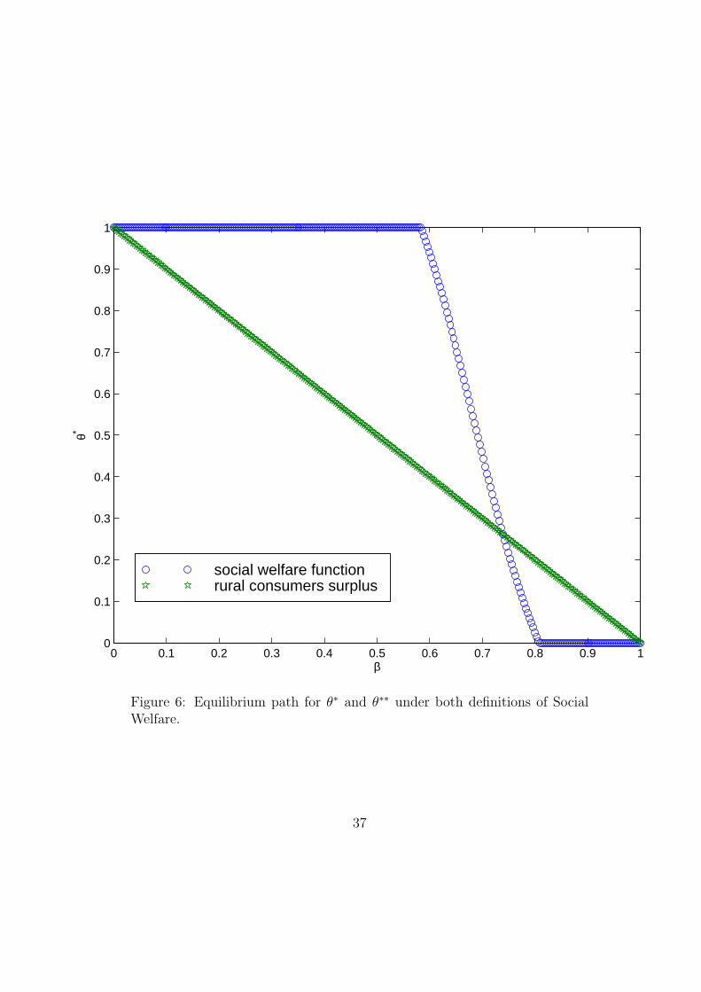
When the second definition is at work, she only takes interior values for θ,because she is not internalizing the U market consumers prices. By definition,the U market prices are one higher and the other lower than the R marketprice. Thus, when the R market is not very large, the regulator is interestingin setting the Cournot price in the largest U market area, what is very oftenachieved choosing a corner solution. Either θ = 0 or θ = 1. By contrast,under SW2 no area of the R market can hold the Cournot price, makingθ ∈ (0, 1) the optimal choice, see figure 6.

Regarding the comparison with the European and American definitionsof affordable prices, it is easy to see that this definition is superior from awelfare viewpoint. As the regulator takes always interior solution for θ, thismeans that she always chooses a better choice than min{pUA

1 , pUA2 }(either

θ = 0 or θ = 1), because it is an available option for her and he does notchoose it.

33We refer only to the European definition, because we have proved that the Europeandefinition is superior in terms of social welfare to the American definition.

18

5 An alternative definition (II): yardstick pric-

ing

We introduce a second new definition of affordable prices. We propose thatthe price in any of the R market areas has to be lower or equal than a functionof the prices in the U market areas excluding the price of the U market areait is attached to.34 If we apply this definition to our model, the price of theareas 1 and 2 of the R market cannot be higher than the price in the areas 2and 1 of the U market respectively, pR

j ≤ pUk , for j = 1, 2, such that k 6= j.35

Once we have described our new definition of prices for the R marketareas, we introduce it into our game in the third stage and we start solvingthe game by backward induction. So, first, we figure out the prices set bythe firms for the different areas of the R market. The constraint pR

j ≤ pUk ,

for j = 1, 2 such that k 6= j is binding in equilibrium. The monopoly pricein any R market area is always higher than the equilibrium prices of any Umarket area. Thus, pR

j = pUk , k 6= j.

The second stage is to find the equilibrium quantities in the U marketareas. The prices in the U market areas are determined by:

pUj = (1− (qSj + qNj)

αj

), j = 1, 2.

Given this and pRj = pU

k for j = 1, 2, such that k 6= j, the profits of thefirms that operate in both areas j of the U and R markets are:

Π1j = (1− (qSj + qNj)

αj

)qSj+

+(1− ((qSk + qNk)

αk

))(βjb(qSk + qNk)

αk

)− FUj − FR

j + sj,

j = 1, 2, k 6= j.

34This definition is inspired in the concept of ”yardstick competition”, as defined inShleifer (1985).

35If we extend our model to N areas in the R and U markets, pRj ≤

f(pU1 , ...., pU

j−1, pUj+1, ...P

UN ), j = 1, ..., N . The most likely functional form for f(.) would

be the sample mean of all prices expect pUj .

19

The profits of the firms that only operate in the areas of the U marketare:

ΠNj = (1− (qSj + qNj)

αj

− c)qNj − FUj , j = 1, 2.

Given all profit functions, if we maximize them, we obtain the followingresult:

Proposition 8 Under yardstick pricing, the symmetric Cournot price, pC =13, is set in the whole R and U markets.

With this new regulation, we can set the lowest possible price in the wholecountry, given that firms compete a la Cournot in their respective areas ofthe U market. We have reached such a good result for the social welfarebecause we were able to break the strategic link that the American and theEuropean definition of affordable prices create between the areas of the Uand R markets. This strategic link made the equilibrium prices higher thanthe symmetric Cournot price.36

This regulatory regime has a negative aspect. In order to be worthyto apply it, we need that the differences in demand between the differentzones of the country be small enough. For example, consider a situationwhere the demands in areas 1 and 2 of the U market are DU

1 (p) = 1 − pand DU

2 (p) = (a − p) the demand in area 1 and 2 of the R market areDR

1 (p) = b(1 − p) and DR2 (p) = b(a − p) where a < 1.37 If we apply the

proposed definition, we find that the symmetric Cournot equilibrium for thearea 1 of the U market is pC = 1

3, which is even bigger than the monopoly

price in the area 2 of the U market if a < 23.38

6 Conclusions

In this paper, we have analyzed different definitions of affordable prices underUniversal Service Obligations focusing on their implications on social welfare.

36For further details, see Anton et al. (2002) or Valletti et al. (2002).37This could describe a situation where the R market consumers are poorer than the U

area consumers.38This may happen in Spain or Italy if we divide the countries in such a way that the

zone 1 is the northern half of the countries (richer) and zone 2 is the southern half of thecountries (poorer).

20

We have studied the different definitions under the assumption that a countryis divided into independent zones. Each of these zones consists on a profitableand an unprofitable area.

We have studied first, the definition of affordable prices that come fromthe American and the European regulatory regimes. The American regu-latory regime advocates for a common price within each zone, whereas theEuropean regulatory regime advocates for a common price for the wholecountry. We have shown that these two definitions of affordable prices areequivalent when the zones are designed in such a way that the ratio betweenthe demands of the areas within each zone is constant. If this does nothappen, the European definition is social welfare superior to the Americandefinition. This is because the European definition obliges to set a uniqueprice in the country.

We have also presented two new definitions of affordable prices. In thefirst definition, the price in all the unprofitable markets is the same and itcannot be higher than a convex combination of the prices in the profitableareas. We have proved that this definition is always social welfare superiorto the European definition, and by extension to the American. Under thisdefinition, when the welfare function is the standard, in many cases, theregulator chooses the maximum or the minimum of the available prices toapply it to the unprofitable market. This implies that there are profitableareas which enjoy the symmetric Cournot price (the lowest in our context). Inthe other cases, the regulator chooses convex combinations of the unprofitablemarket areas prices. It may sound strange that when the regulator opts forthe maximum, this definition can be superior to the European definition.This is so, because under some circumstances (when the total unprofitabledemand is small compared to the total demand), the best for social welfare isto set the symmetric Cournot price to as many consumers as possible in theprofitable market, and to do so, the regulator has to impose the maximum.When the welfare function is only the unprofitable consumers surplus, theregulator choices change and she only chooses convex combinations of theunprofitable market area prices. This is for two reasons. First, becausethe unprofitable market consumers enjoy different prices than the profitablemarket consumers, and second, because the regulator does not internalizethe profitable market consumers surplus.

The other definition we have presented is what we denote ”yardstick pric-ing”. In this definition, the prices of the unprofitable areas can never behigher than a function of the prices of all profitable areas expect the price

21

of its own zone profitable area. With this definition, we break the strategiclink that firms use to raise the price. Thus, we can implement the symmetricCournot price all over the country which yields the maximum social welfare.The problem with this last definition is that to work properly we need con-sumers’ demands not to be very different between the different zones. Forexample, this definition can yield very bad results from a social point of viewwhen the differences in income between zones are very high.

Given our results. National Regulatory Board should implement our firstdefinition when differences in demand between markets are very large, andyardstick pricing when the differences are not significant.

22

References

[1] Anton J.J., Vander J.H. and Vettas N. (2002). ”Entry auctions andstrategic behavior under cross-market price constraints. InternationalJournal of Industrial Organization, vol 20, pp 611-629.

[2] Chone P., Flochel L. and Perrot A. (2000). ”Universal service obligationsand competition”. Information Economics and Policy. vol 12(3). pp 249-259.

[3] Chone P., Flochel L. and Perrot A. (2002). ”Allocating and funding uni-versal service obligations in a competitive market”. International Journalof Industrial Organization. vol 20(9). pp 1247-1276.

[4] European Parliament and the Council of the European Union. (2002).”Directive 2002/22/CE”

[5] Federal Communication Commission (1996). ”Telecommunication Act”

[6] Federal Communication Commission (1996). ”In the matter of Federal-State Joint Board on Universal Service”. CC Docket no 96-47.

[7] Gasmi F., Laffont J.J. and Sharkey W.W. (2000). ”Competition, uni-versal service and telecommunication policy in developing countries”.Infomation Economics and Policy, vol 12(3), pp 221-248.

[8] Iozzi. A. (2001). ”Who gains from Universal Service Obligations? A wel-fare analysis of the rule ’One price for everywhere’”. Studi Economici,vol 74(2), pp 131-152.

[9] Laffont J.J. and Tirole J. (2000). ”Competition in Telecommunications”.Cambridge, MA, MIT Press.

[10] Rosston G. and Bradley S. (2000). ”The ’state’ of universal service”Information Economics and Policy, vol 12(3), pp 261-283.

[11] Shleifer A. (1985). ”A theory of yardstick competition” RAND Journalof Economics, vol 16(3), pp 319-327.

[12] Valletti T. (2000). ”Introduction: Symposium on universal service obli-gation and competition” Information Economics and Policy, vol 12(3),pp 205-210.

23

[13] Valletti T., Hoernig S. and Barros P.P. (2002). ”Universal Service andEntry: The Role Of Uniform Pricing and Coverage Constraints”. Jour-nal of Regulatory Economics, vol 21(2), pp 169-190.

24

A appendix

A.1 Proof Proposition 1

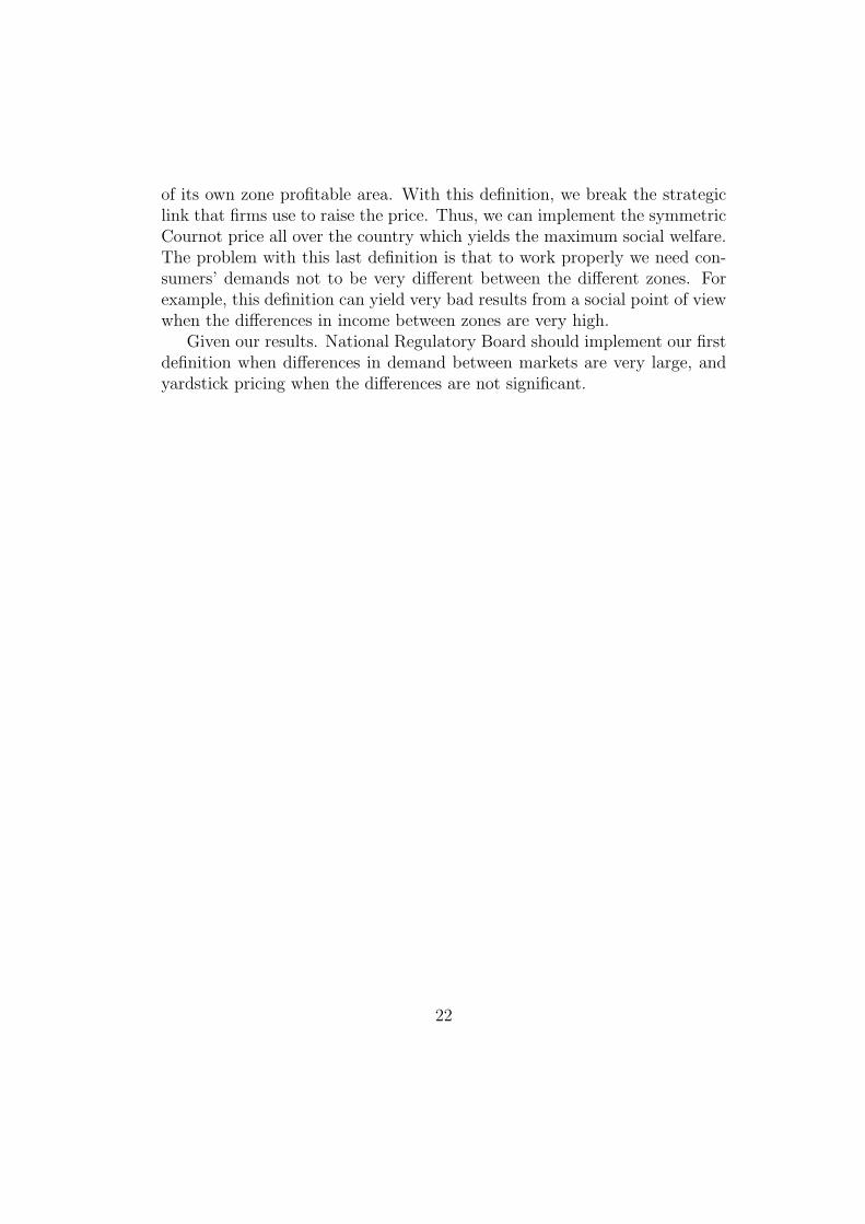
We first show the result under the proviso that the regulator maximizes SW1.In this case, she chooses α1 and β1 as to:

maxα1,β1

SW1(α1, β1) = (α1 + bβ1)(1− pUA

1 (α1, β1))2

2+

((1−α1)+b(1−β1))(1− pUA

2 (α1, β1))2

2+(α1+bβ1)p

UA1 (α1, β1)(1−pUA

1 (α1, β1))+

+((1− α1) + b(1− β1))pUA2 (α1, β1)(1− pUA

2 (α1, β1)),

where the first two terms are consumers surplus and the remaining twoterms are firms profits.

Now,

pUA1 (α1, β1) =

α1 + β1b

3α1 + 2β1b

is the price in area 1 of the U market under the American regulation, and

pUA2 (α1, β1) =

(1− α1) + (1− β1)b

3(1− α1) + 2(1− β1)b

is the price in area 2 of the U market under the American regulation.Differentiating the social welfare function with respect to α1 and β1 we

have:

∂SW1(α1, β1)

∂α1

=(1− pUA

1 (α1, β1))2

2−(α1+bβ1)(1−pUA

1 (α1, β1))∂pUA

1 (α1, β1)

∂α1

−

(1− pUA2 (α1, β1))

2

2− ((1− α1) + b(1− β1))(1− pUA

2 (α1, β1))∂pUA

2 (α1, β2)

∂α1

+

pUA1 (α1, β1)(1− pUA

1 (α1, β1)) + (α1 + bβ1)(∂pUA

1 (α1, β1)

∂α1

(1− pUA1 (α1, β1)))−

25

(α1 + bβ1)(pUA1 (α1, β1)

∂pUA1 (α1, β1)

∂α1

)− pUA2 (α1, β1)(1− pUA

2 (α1, β1))+

((1− α1) + b(1− β1))(∂pUA

2 (α1, β1)

∂α1

(1− p2(α1, β2)))

−((1− α1) + b(1− β1))(pUA2 (α1, β1)(

∂pUA2 (α1, β1)

∂α1

),

and

∂W (α1, β1)

∂β1

= b(1− pUA

1 (α1, β1))2

2− (α1 + bβ1)(1−pUA

1 (α1, β1))∂pUA

1 (α1, β1)

∂β1

−b(1− pUA

2 (α1, β1))2

2− ((1−α1)+ b(1−β1))(1− pUA

2 (α1, β1))∂pUA

2 (α1, β2)

∂β1

+

bpUA1 (α1, β1)(1− pUA

1 (α1, β1)) + (α1 + bβ1)(∂pUA

1 (α1, β1)

∂β1

(1− pUA1 (α1, β1)))

−(α1 + bβ1)(pUA1 (α1, β1)

∂pUA1 (β1, β1)

∂β1

)− bpUA2 (α1, β1)(1− pUA

2 (α1, β1))+

((1− α1) + b(1− β1))(∂pUA

2 (α1, β1)

∂β1

(1− p2(α1, β2)))

−((1− α1) + b(1− β1))(pUA2 (α1, β1)(

∂pUA2 (α1, β1)

∂β1

).

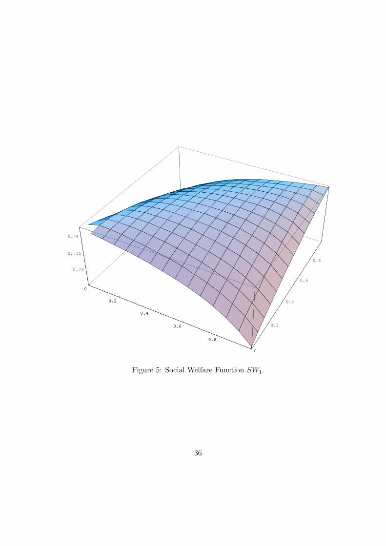
Both derivatives equal zero at α1 = β1. Since, further, the function isconcave in both variables, see figure 5, we can conclude that α1 = β1 are themaxima of the social welfare function.

26

We now analyze the regulator choice when she maximizes SW2. Theprogramme she faces is to maximize

bβ1(1− pUA

1 (α1, β1))2

2+ b(1− β1)

(1− pUA2 (α1, β1))

2

2,

where the social welfare function is the sum of the consumers’ surplus inthe R market.

Differentiating the social welfare function with respect to α1 and β1 wehave:

∂SW2(α1, β1)

∂α1

= β1b(1−p1(α1, β1))∂p1(α1, β1)

∂α1

+(1−β1)b(1−p2(α1, β1))∂p2(α1, β1)

∂α1

and

∂SW2(α1, β1)

∂β1

= b(1− p1(α1, β1))

2

2+ β1b(1− p1(α1, β1))

∂p1(α1, β1)

∂β1

−b(1− p1(α1, β1)

2

2+ (1− β1)b(1− p2(α1, β1))

∂p2(α1, β1)

∂β1

.

As for the other social welfare function, both derivatives equal 0 at α1 =β1. As the function is concave, α1 = β1 are maxima.

A.2 Proof Proposition 2

If α1

β1= 1 then α2

β2= 1 as well, as α1 + α2 = 1 and β1 + β2 = 1. Given the

equilibrium prices under the American definition:

pUAj =

(αj + βjb)

3αj + 2βjb, j = 1, 2

The following condition has to hold in order to ensure that they are equal:

α1 + β1b

3α1 + 2β1b=

α2 + β2b

3α2 + 2β2b.

Note that α1/β1 = α2/β2 = 1 is a sufficient condition to guarantee thatthey are equal as:

1 + b

3 + 2b=

1 + b

3 + 2b.

27

A.3 Proof Proposition 3

We know that the price-cap pRj ≤ pU

j , j = 1, 2 is binding in equilibrium.This means that within each zone, there is a unique price. If we introducethe price-cap pU

j ≤ min{pUA1 , pUA

2 }, we can guarantee that it is also bindingin equilibrium by the definition of minimum. This means that both zonesshare the same prices.

A.4 Proof Proposition 4

The proof under SW1 goes as follows: under the European definition, min{pUA1 , pUA

2 }is applied to all areas of the U and R markets. Assuming without loss of gen-erality that min{pUA

1 , pUA2 } = pUA

1 , the weighted price for the whole countrybecomes:

α1pUA1 + α2p

UA1 + β1bp

UA1 + β2p

UA1 .

Under the American definition zone 1 enjoys price pUA1 and zone 2 enjoys

price pU2A. Thus, the weighted price for the whole country is:

α1pUA1 + α2p

UA2 + β1bp

UA1 + β2p

UA2

The European definition is social welfare superior when the weighted pricefor the whole country is lower under this definition than under the Americandefinition, i.e., when the inequality below holds:

α1pUA1 + α2p

UA1 + β1bp

UA1 + β2p

UA1 < α1p

UA1 + α2p

UA2 + β1bp

UA1 + β2p

UA2

or, rearranging, when:

pUA1 < pUA

2

which is true by the assumption of min{pUA1 , pUA

2 } = pUA1 .

Under SW2, it is trivial that the same result holds. We only need toremove U market areas sizes from the weighted prices, and we see easilythat the weighted prices under European definition is lower than under theAmerican definition.

28

A.5 Proof Proposition 5

Under SW1, the regulator chooses θ to maximize:

α1(1− pU

1 (θ))2

2+ α2

(1− pU2 (θ))2

2+ b

(1− pR(θ))2

2+ α1p

U1 (θ)(1− pU

1 (θ))+

+α2pU2 (θ)(1− pU

2 (θ)) + bpR(θ)(1− pR(θ))

where the first three terms are the consumers’ surpluses from areas 1 and2 of the U market and R market respectively, and the last two terms are theprofits of firms, and where

pU1 (θ) =

α1(3α2 + 2bβ2(1− θ)2) + α2bβ1θ(1 + 2θ)

3(α1(3α2 + 2bβ2(1− θ)2) + 2α2bβ1θ2),

is the price in area 1 of the U market,

pU2 (θ) =

α1(α2 + bβ2(3− 5θ + 2θ2)) + 2α2bβ1θ2

3(α1(3α2 + 2bβ2(1− θ)2) + 2α2bβ1θ2),

is the price in area 2 of the R market, and

pR(θ) =α1(α2 + bβ2(1− θ)2) + α2bβ1θ

2)

3(α1(3α2 + 2bβ2(1− θ)2) + 2α2bβ1θ2),

is the price in the R market. Recall further that α1 + α2 = 1, andβ1 + β2 = 1.

Differentiating the social welfare function, we have:

∂SW1(θ)

∂θ= −α1(1−pU

1 (θ))∂pU

1 (θ)

∂θ−α2(1−pU

2 (θ))∂pU

2 (θ)

∂θ−b(1−pR(θ))

∂pR(θ)

∂θ+

+α1(1− pU1 (θ))

∂pU1 (θ)

∂θ+ α2(1− pU

2 (θ))∂pU

2 (θ)

∂θ+ b(1− pR(θ))

∂pR(θ)

∂θ−

−α1pU1 (θ)

∂pU1 (θ)

∂θ− α2p

U2 (θ)

∂pU2 (θ)

∂θ− bpR(θ)

∂pR(θ)

∂θ= 0

Straightforward computations result in the first order conditions for max-imum:

29

∂W (θ)

∂θ= −α1p

U1 (θ)

∂pU1 (θ)

∂θ− α2p

U2 (θ)

∂pU2 (θ)

∂θ− bpR(θ)

∂pR(θ)

∂θ= 0

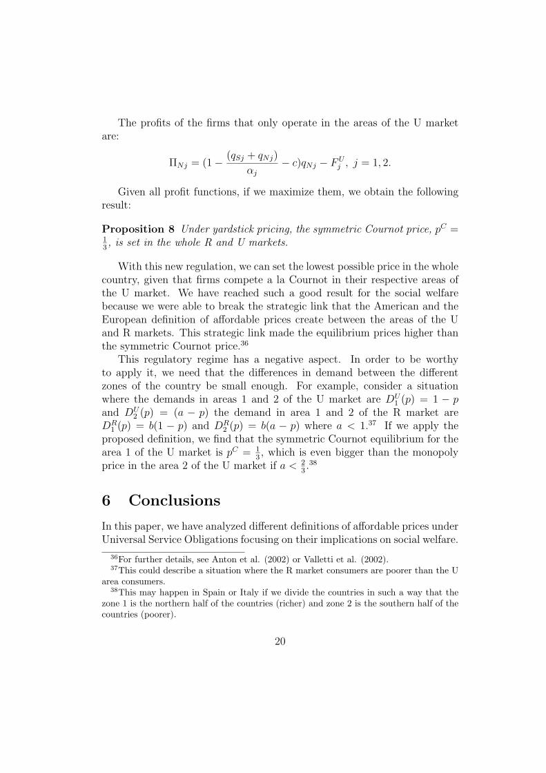
From this first order condition, we cannot obtain a close form solutionfor θ. Nevertheless, numerical resolution shows that for given α1 and b, theoptimum for θ is unique. Further, we get

1. θ∗ = 1 if β1 ∈ [0, β1]

2. θ∗ = 0 if β1 ∈ [β1]

3. θ∗ ∈ (0, 1) if β1 ∈ [β1, β1]

as it is shown in figure 3 and 4. From figure 3, we can also see how β1

and β1 are increasing function of α1. From figure 4, we can see that β1 is

an increasing function of b while β1 is a decreasing function of b. Finally, wehave checked that these optima are indeed maxima.

A.6 Proof Proposition 6

Under SW2 the regulator’s objective function becomes:

SW2(θ) = b(1− pR(θ))2

2

Solving the first order condition for maximum we get:

∂SW2(θ)

∂θ= b(1− pR(θ))

∂pR(θ)

∂(θ)= 0 ⇒ θ∗∗ =

α1(1− β1)

(1− α1)β1 + α1(1− β1

.

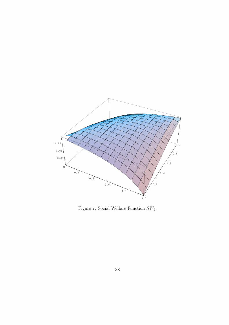
Since SW2(θ) is a concave function as we can see in Figure 7, we canconclude that θ∗∗ is an optimal solution.

A.7 Proof Proposition 7

We start from the case when in equilibrium pR = min{pUA1 , pUA

2 } and wesuppose that min{pUA

1 , pUA2 } = pUA

1 . Therefore areas 1 and 2 of the R marketenjoy a price pUA

1 , as well as area 1 of the U market. Area 2 of the R

30

market enjoys the symmetric Cournot price which is lower than pUA1 . We can

construct a weighted price for the whole country under this definition:

α1pUA1 + α2p

C + bpUA1 .

where pC is the symmetric Cournot price. On the other hand, the Euro-pean definition applies pUA

1 to the whole country. Thus, the weighted pricefor the whole country is:

α1pUA1 + α2p

UA1 + bpUA

1 .

The new definition is superior in terms of social welfare if it gives a lowerweighted price than the European definition. This happens if

α1pUA1 + α2p

C + bpUA1 < α1p

UA1 + α2p

UA1 + bpUA

1

or equivalently, if pC < pUA1 , what is true. Therefore, the new definition

is superior to the European definition, whenever we apply min{pUA1 , pUA

2 }. Ifwe take into account that we only apply either max{pUA

1 , pUA2 } or θ∗ ∈ (0, 1)

when they are social welfare superior to min{pUA1 , pUA

2 }, we can conclude thatthis definition is always social welfare superior to the European definition,and by extension to the American as we have shown previously.

A.8 Proof Proposition 8

The firms that operate in both areas maximize:

ΠSj = (1− (qSj + qNj)

αj

)qSj+

(1− ((qSk + qNk)

αk

)− c)(βjb(qSk + qNk)

αk

)− FUj − FR

j + sj

j = 1, 2, k 6= j.

If we take the derivative of the profit function with respect to q1j, weobtain the first order conditions:

31

∂ΠSj

∂qsj

= (1− (2qSj + qNj

αj

)) = 0, j = 1, 2

The firms that only operate in the areas of the U market maximize:

ΠNj = (1− (qSj + qNj)

αj

)qNj − FUj , j = 1, 2

If we take the derivative of the profit function with respect to qNj, weobtain the first order conditions:

∂ΠNj

∂qNj

= (1− (qSj + 2qNj

αj

)) = 0, j = 1, 2

These first order conditions yield the following equilibrium quantities:

q∗Sj =αj

3, q∗Nj =

αj

3, j = 1, 2

If we substitute the equilibrium quantities in the demand function, weobtain the equilibrium price for the areas of the U market which is the sym-metric Cournot price:

pU∗j = (1− q∗Sj + q∗Nj

αj

) =1

3, j = 1, 2

As we have seen previously, the prices in the zones are the same for bothareas, therefore, the symmetric Cournot price is also set in the areas of theR market.

32

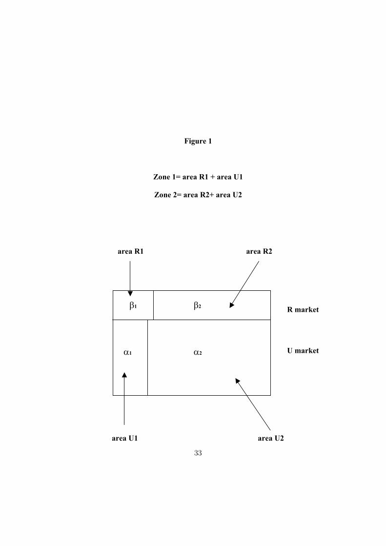
Figure 1

Zone 1= area R1 + area U1

Zone 2= area R2+ area U2

R market

U market

area U2 area U1

1 2

21

area R1 area R2

Figure 1: Example of a country divided in zones

33

1

0.5

0.5

b=0.5

b=4

min

min

max

0

1

Figure 2: The regulator optimal choice between max{pUA1 , pUA

2 } andmin{pUA

1 , pUA2 }

34

0 0.1 0.2 0.3 0.4 0.5 0.6 0.7 0.8 0.9 10

0.1

0.2

0.3

0.4

0.5

0.6

0.7

0.8

0.9

1

β1

θ*

α1=0.25, b=0.5

α1=0.5, b=0.5

α1=0.75, b=0.5

Figure 3: Equilibrium path for θ∗ under different values of α1.

0 0.1 0.2 0.3 0.4 0.5 0.6 0.7 0.8 0.9 10

0.1

0.2

0.3

0.4

0.5

0.6

0.7

0.8

0.9

1

β1

θ*

α1=0.5, b=0.5

α1=0.5, b=0.75

Figure 4: Equilibrium path for θ∗ under different values of b.

35

0

0.2

0.4

0.6

0.8

0

0.2

0.4

0.6

0.8

0.73

0.735

0.74

0

0.2

0.4

0.6

0.8

Figure 5: Social Welfare Function SW1.

36

0 0.1 0.2 0.3 0.4 0.5 0.6 0.7 0.8 0.9 10

0.1

0.2

0.3

0.4

0.5

0.6

0.7

0.8

0.9

1

θ*

β

social welfare functionrural consumers surplus

Figure 6: Equilibrium path for θ∗ and θ∗∗ under both definitions of SocialWelfare.

37

0

0.2

0.4

0.6

0.8

1 0

0.2

0.4

0.6

0.8

1

0.07

0.08

0.09

0

0.2

0.4

0.6

0.8

Figure 7: Social Welfare Function SW2.

38