On the difficulty to optimally implement the Ensemble Kalman Filter: Anexperiment based on many hydrological models and catchments

A. Thiboulta,∗, F. Anctila

aDept. of Civil and Water Engineering, Universite Laval, Quebec, Canada

Published in Journal of Hydrology 529 (2015) 1147–1160https://doi.org/10.1016/j.jhydrol.2015.09.036

Abstract

Forecast reliability and accuracy is a prerequisite for successful hydrological applications. This aim may be attained by usingdata assimilation techniques such as the popular Ensemble Kalman filter (EnKF). Despite its recognized capacity to enhanceforecasting by creating a new set of initial conditions, implementation tests have been mostly carried out with a single modeland few catchments leading to case specific conclusions. This paper performs an extensive testing to assess ensemble bias andreliability on 20 conceptual lumped models and 38 catchments in the Province of Quebec with perfect meteorological forecastforcing. The study confirms that EnKF is a powerful tool for short range forecasting but also that it requires a more subtle settingthan it is frequently recommended. The success of the updating procedure depends to a great extent on the specification of thehyper-parameters. In the implementation of the EnKF, the identification of the hyper-parameters is very unintuitive if the modelerror is not explicitly accounted for and best estimates of forcing and observation error lead to overconfident forecasts. It is shownthat performance are also related to the choice of updated state variables and that all states variables should not systematically beupdated. Additionally, the improvement over the open loop scheme depends on the watershed and hydrological model structure, assome models exhibit a poor compatibility with EnKF updating. Thus, it is not possible to conclude in detail on a single ideal mannerto identify an optimal implementation; conclusions drawn from a unique event, catchment, or model are likely to be misleadingsince transferring hyper-parameters from a case to another may be hazardous. Finally, achieving reliability and bias jointly is adaunting challenge as the optimization of one score is done at the cost of the other.

Keywords:Data assimilation, Uncertainty estimation, Ensemble Kalman filter

1. Introduction

Despite the modelling advances in representing hydrologicalprocesses and providing more accurate streamflow forecasts,there is still a need for reducing and quantifying uncertainty.Most hydrological prediction systems are still deterministicand provide only the most likely outcome without addressingestimates of their uncertainty. The sources of uncertainty stemfrom multiple places in the hydrometeorological chain suchas in inputs, initial conditions, parameter estimation, modelstructure, and outputs (e.g. Ajami et al., 2007; Salamon andFeyen, 2010; Liu and Gupta, 2007; Liu et al., 2012) and theseuncertainties should be deciphered to enhance model predictiveabilities and reliability for efficient decision making (Ramoset al., 2010).

A broad range of techniques has been developed to con-trol uncertainty at different levels such as the GeneralizedLikelihood Uncertainty Estimation (GLUE), Shuffle ComplexEvolution Metropolis algorithm (SCEM) for parameter uncer-tainty (Beven and Binley, 1992; Vrugt et al., 2003) and BMA

∗Corresponding authorEmail address: antoine.thiboult.1@ulaval.ca (A. Thiboult)

combination technique for structural uncertainty (Jeremiahet al., 2011; Duan et al., 2007; Parrish et al., 2012; Ajamiet al., 2007). Proper initial conditions are frequently identifiedas one of the main factors that contributes to an accurateforecast (DeChant and Moradkhani, 2011; Lee et al., 2011).Among others, data assimilation (DA) is commonly used inhydrometeorology to reduce initial condition uncertainty andproved to be a useful tool for modelling. DA incorporatesobservations into the numerical model to issue an analysis,which is an estimation of the best current state of the system.This has not only been largely applied to remote sensingfor snow (Kuchment et al., 2010), soil moisture estimates(Forman et al., 2012; Meier et al., 2011; Renzullo et al., 2014;Alvarez-Garreton et al., 2014) or hydraulic information (Baileyand Bau, 2012), but also to update radar forcing (Haraderet al., 2012; Kim and Yoo, 2014). Many applications also usein situ observations such as catchment discharge, snowpackmeasurements, or soil moisture to update models (e.g., Seoet al., 2009; Clark et al., 2008; Thirel et al., 2010; DeChant andMoradkhani, 2011; Franz et al., 2014). In addition, DA maybe coupled with parameter optimization (Vrugt et al., 2005;Moradkhani et al., 2005; Nie et al., 2011).

Preprint: Published in Journal of Hydrology November 27, 2017

Sequential DA techniques such as particle filter and theKalman filter family are frequently used for recursive updatingof the states of a system, each time an observation is madeavailable. Among them, the ensemble Kalman filter (EnKF,Evensen, 1994) proved to be a powerful tool for hydrologicalforecasting (DeChant and Moradkhani, 2012; Rakovec et al.,2012; Vrugt and Robinson, 2007; Weerts and El Serafy, 2006;Abaza et al., 2014) that is effective and reliable enough foroperational use (Andreadis and Lettenmaier, 2006). Severalstudies claim that they developed techniques that improvedupon traditional EnKF (e.g., Clark et al., 2008; Whitaker andHamill, 2002) by focusing on the relaxation of constrains oftraditional EnKF implementation, or by explicitly includingtime lag between the soil moisture and the discharge in theupdating process (Li et al., 2013, 2014; McMillan et al., 2013).

A key feature of EnKF is the proper specification of hyper-parameters (perturbations of inputs and outputs) and modelstates to be updated (Moradkhani et al., 2005). In most stud-ies, EnKF implementation is based on an a priori selection ofthe hyper-parameters and updated states combination, which isthen scarcely justified. Noteworthy exceptions are Moradkhaniet al. (2005) and Chen et al. (2013), but these studies are veryspecific as they are performed on a single model and one ortwo catchments. Accurate perturbations representing error esti-mates are crucial since the EnKF updating scheme is based onthe weighting of the model and observation relative error. How-ever this specification is complex in practice as the differentsources of uncertainty experience strong interactions (Morad-khani et al., 2006; Hong et al., 2006; Kuczera et al., 2006). Sev-eral attempts to account explicitly for structural error have beenreported, for example by directly adding perturbations to thestate variables (Reichle et al., 2002; Vrugt et al., 2006; Clarket al., 2008), or by updating model parameters (Moradkhaniet al., 2005; Vrugt et al., 2005; Naevdal et al., 2003).

Moreover, despite encouraging results, DeChant and Morad-khani (2012) point that little research has been done to examinethe effectiveness and robustness of EnKF and that ”studiesneed to provide a more rigorous testing of these techniquesthan has previously been presented”. Another issue that needsconsideration is that EnKF performance is mostly discussed as’standalone’, regardless of the influence of the coupling withthe hydrological model. This is mainly due to the fact thatEnKF is often tested on a single model. Thus, the question ofadequacy between the DA technique and the model is rarelyassessed.

The present study aims at identifying EnKF parametrizationto reduce and quantify optimally the uncertainty related toinitial conditions in a forecast mode. A second scope addressesthe question of EnKF and hydrological model adequacy. In or-der to achieve this, the analysis is conducted on 20 structurallydissimilar lumped conceptual models, 38 catchments, 12hyper-parameter sets, and all possible combinations of the statevariables to strive for general results. Finally, the effectivenessof identifying the best EnKF parametrization without exploringall combinations is discussed.

Section 2 presents EnKF’s basics, models, basins and scores.Section 3 presents the results of the DA techniques followedby a discussion and the conclusion statements are provided insection 4.

2. Material and methods

2.1. Hydrological models, snowmelt modules, and PET

The EnKF is tested individually on 20 lumped conceptualmodels, which differ by their structure. The selection wasinitially carried out by Perrin (2000) and revised by Seiller et al.(2012) for hydrological projection purposes. Because they arebased on diverse hydrological concepts and present differentdegrees of complexity (4 to 10 calibrated parameters and 2 to7 reservoirs to represent perceptual and conceptual hydrologicprocesses), they allow to test the EnKF in a comprehensivemanner according to structure diversity (see Table 1). Themodels have been modified to match a common frame andthey should not be directly compared to their original version.In the case where the original models included a module tocompute evapotranspiration or snow accumulation and melting,the module has been omitted as these processes are computedexternally beforehand.

The models exploit various conceptualizations and thustheir parameters and state variables perform particular rolesin simulating rainfall-runoff processes. Their reservoirs maydescribe systems ranging from precipitation interception torouting (or more conceptual functions). The role of statevariables is not detailed in the article for concision purpose.For the same reason, the state variable values before and afterthe analysis step will not be discussed here but only the outputsof the models, i.e., simulated streamflow will be considered.For further details on state variable meaning, refer to Perrin(2000).

The lumped models are driven by potential evapotranspi-ration and precipitation. The potential evapotranspiration iscomputed from the formula proposed by Oudin et al. (2005),which relies on mean air temperature and the calculatedextraterrestrial radiation. To partition snow accumulation,snowmelt, and liquid precipitation, the snow module (Ce-maneige, Valery et al., 2014) is executed before hydrologicalmodels.

The snow module divides the watershed into 5 elevationbands and is based on a degree-day approach modulated by anenergy balance index to simulate the dynamic of the snowpack.

The models are calibrated with the Shuffle Complex Evo-lution algorithm (Duan et al., 1992) and the RMS E is usedon square-rooted streamflows as objective function to ensurethat calibration does not favor either low or high streamflows.Each of the 20 models is calibrated individually with the2-parameter snow module — the parameter values of the snow

2

Table 1: Main characteristics of the 20 lumped models (Seiller et al., 2012)Model No of No of Derived fromacronym param. reserv.M01 6 3 BUCKET (Thornthwaite and

Mather, 1955)M02 9 2 CEQUEAU (Girard et al.,

1972)M03 6 3 CREC (Cormary and Guilbot)M04 6 3 GARDENIA (Thiery, 1982)M05 4 2 GR4J (Perrin et al., 2003)M06 9 3 HBV (Bergstrom and Forsman,

1973)M07 6 5 HYMOD (Wagener et al.,

2001)M08 7 3 IHACRES (Jakeman et al.,

1990)M09 7 4 MARTINE (Mazenc et al.,

1984)M10 7 2 MOHYSE (Fortin and Turcotte,

2007)M11 6 4 MORDOR (Garcon, 1999)M12 10 7 NAM (Nielsen and Hansen,

1973)M13 8 4 PDM (Moore and Clarke, 1981)M14 9 5 SACRAMENTO (Burnash

et al., 1973)M15 8 3 SIMHYD (Chiew et al., 2002)M16 8 3 SMAR (O’Connell et al., 1970)M17 7 4 TANK (Sugawara, 1979)M18 7 3 TOPMODEL (Beven et al.,

1984)M19 8 3 WAGENINGEN (Warmerdam

et al., 1997)M20 8 4 XINANJIANG (Zhao et al.,

1980)

module are consequently different for each hydrological model.

2.2. Experimental design, state updating, and EnKF imple-mentation

EnKF addresses explicitly initial conditions uncertainty bycreating an ensemble of possible model reinitializations byupdating state variables according to a recursive Bayesianestimation scheme. It estimates the true probability densityfunction of the model states conditioned by the observations.

The evolution of the model state variables vector x may bedescribed through time with a non-linear forward operator Mdriven by the previous states, the deterministic forcing u thatincludes an error term ζt, and the (time-invariant) model param-eters θ to which a model error η is added. The η error term doesnot include only state variable error but also implicitly othersources of error such as the structural and parameter error orforcing error.

xt = M(xt−1, ut−1, θ) + ηt (1)

States and observations z are related through the following ex-pression

zt = H(xt) + εt (2)

with H being the observation function and εt the observationerror.

The EnKF relies on an approximation of Bayesian rule toidentify the conditional density of the model states, p(xt |z1:t),given the previous time steps observations z1:t, where xt is thestate vector that contains the model states. EnKF needs severalrealisations (N members) to derive the model error matrix. Asthe real true state is unknown, it is approximated by the ensem-ble mean :

xt =1N

N∑i=1

xit (3)

where i refers to the ith member. The model error matrix is thusdefined as the difference between the true state and the singlehydrological model realisations:

Et = (x1t − xt, x2

t − xt, ..., xNt − xt) (4)

Therefore, the model covariance matrix can be defined as:

Pt =1

N − 1EtET

t (5)

When an observation is available, model states are updated (X+)as a combination of the prior states X− and the difference be-tween the prior estimate HtX−t and observation.

X+t = X−t + Kt(zt −HtX−t ) (6)

The Kalman gain Kt represents the relative importance of theobservation error with respect to the prior estimate (i.e. modelsimulation) and acts as a weighting coefficient. Rt denotes thecovariance of the observational noise.

Kt = PtHTt (HtPtHT

t + Rt)−1 (7)

Since the identification of the Kalman gain is complex, the termPtHT

t is approximated by the forecasted covariance between themodel states and the simulation estimates and HtPtHT

t by thevariance of the estimate.

PtHTt =

1N − 1

N∑i=1

(xit − xt)(Ht xi

t −Ht xt)T (8)

HtPtHTt =

1N − 1

N∑i=1

(Ht xit −Ht xt)(Ht xi

t −Ht xt)T (9)

A more detailed description of EnKF equations and math-ematical background can be found in Evensen (2003). In thisstudy, the filter has been implemented following Mandel’s(2006) computational recommendations.

A critical point in the EnKF implementation is a propermapping of the errors ε, ζ, and η because they will determinethe observation predictive distribution. In a very vast majority

3

of cases, model error is not directly identifiable. Users needto estimate it by using stochastic perturbations through ε andζ computation if no more direct estimation of model error η ismade through perturbation of states or updating state variableand parameters conjointly. Note that adding perturbations tostates and parameter updating are also subject to inaccuraciessince they are ”based on order-of-magnitude considerations,and may therefore be statistically unreliable” (Liu et al., 2012).In the present study, only ε and ζ are considered. Errors areassumed to be normally distributed with zero mean but theirvariances need to be put under scrutiny.

Hyper-parameters define the statistical properties of the forc-ing and observations ensembles. This study concentrates on theinfluence of the uncertainty in precipitation and temperatureforecasts and in streamflow observation. Three precipitationperturbations (with a standard deviation corresponding to25%, 50%, and 75% of the initial precipitation forecastmagnitude), two streamflow perturbations (with a standarddeviation corresponding to 10% and 25% of the observation),two temperature perturbations (standard deviation of 2oC and5oC) are evaluated. These perturbations are centred around theperfect forecast or the observation. We thus obtain 12 sets ofhyper-parameters. All errors are assumed to be uncorrelated.Note that the potential evapotranspiration is not directlyperturbed but it is computed by the Oudin formula forced witha temperature ensemble creating a subsequent set of perturbedPET values.

The present updating scheme relies on the Markov propertythat asserts that the future of the system is dictated only bythe present state, not on the anterior sequence of observa-tions. Model states are consequently updated according tothe instantaneous covariance between states and the currentstreamflow observation while observations that preceded it arenot incorporated. Li et al. (2013) affirms that this assumptionmay harm updating performance of models that incorporateunit-hydrograph routing but do not affect models that includedynamic routing stores, which is the case for 19 of the 20models used in this study. Only model 5 (GR4J) is based on aunit-hydrograph approach.

Prior to the hyper-parameters evaluation, the number ofmembers composing the EnKF ensemble is investigated. Foursizes (25, 50, 100 and 200 members) are tested on two setsof hyper-parameters. The experiment concerning the numberof members was not conducted on all hyper-parameter sets toreduce computational cost.

The number and the combination of states to be updated arenext put under scrutiny. Batch testing is used to investigate allstates (reservoirs) combinations for each model regardless oftheir physical meaning. The number of possible combinationsthus depends on the model at hand, varying from 3 for the2-reservoir models up to 127 for the 7-reservoir model. Asall combinations of state variables and hyper-parameters aretested, some cases turned out to be unrealistic and prone to

make the EnKF unstable. This difficulty was overcame by set-ting back unrealistic states within their theoretical boundariesidentified during calibration.

The EnKF is used to update daily model’s states wheneverstreamflow observations are available. The model is thenforced with the perfect meteorological forecast to issue a10-day hydrological forecast. This lead time is sufficiently longto be able to see the effect of DA vanishing. A series of tests(not shown here) indicated that after 10 days, the influence ofdata assimilation is almost negligible for almost every modeland catchments. Thus extending the forecast ahead wouldbring no additional information. This framework is comparableto an operational one except for the perfect meteorologicalforcing.

Finally, every 20 models are tested on 38 catchments,12 different hyper-parameter sets, and all possible reservoircombinations.

2.3. ScoresProbabilistic scores offer the possibility to evaluate more

than individual member or ensemble mean and provide to theforecaster a better picture of the forecast probability distribu-tion by expressing the uncertainty level. Probabilistic forecastsshould be assessed both in terms of bias and reliability to assesswhere the verification is situated among the ensemble, how thefrequency of forecasted events corresponds to the frequencyat which events are observed, and the gain of ensemble overdeterministic forecast.

The Normalized Root-mean-square error Ratio (NRR) isused to quantify the spread of the ensemble with regard to itspredictive skills (Murphy, 1988). A value of 1 indicates an ap-propriate spread, while greater and smaller values than 1 reflecttoo narrow and wide ensembles respectively. The NRR is func-tion of the observation yt, the ensemble forecast average ¯yt, thenumber of members in the ensemble N, and time t.

NRR =

√1T

T∑t=1

([1N

N∑n=1

ynt

]− yn

t

)2

1N

N∑n=1

√1T

[T∑

t=1

(yn

t − ynt)2]

√N+12N

(10)

A complementary view of the NRR is the Spread SkillPlot (SSP) which is a graphical assessment that representsat the same time the bias of the ensemble, its spread andtherefore its reliability. The SSP relies on the fact that theRoot-Mean-Square Error (RMSE) should match the spread toachieve reliability (Fortin et al., 2014). In the case where theRMSE is greater than the spread, the ensemble is overconfidentregarding to its predictive skills and vice versa.

The commonly used Nash Sutcliffe efficiency (Nash andSutcliffe, 1970) is used to assess the bias of the median of the

4

EnKF ensemble. A NS E value equals to 1 identifies a perfectprediction while a value below 0 indicates that the averageobservation is more skilful.

To evaluate the improvement or deterioration of the qualityof the simulations, NS E and NRR gains are computed as:

G =S sim − S re f

S opt − S re f (11)

with G the gain, S sim the score after the state updating, S re f

the score without updating (the open loop), and S opt the perfectscore. In the case of the NRR, which is not a monotonic score(i.e. the minimization or maximization of the value does notsystematically indicate an improvement or a decrease of the re-liability), a substitution is performed to compute the gain. Weconsider that under and overdispersion should be penalized thesame way which is reflected by the distance from the optimalscore 1.

NRR∗ = |NRR − 1| (12)

NRR∗ is then negatively oriented and bounded by 0 and can beused to compute the gain G.

2.4. Catchments and hydrometeorological data

38 watersheds are evaluated for this study. They are mainlysituated in the south of the Province of Quebec, but someextend over Ontario or the north of the states of New Yorkand Vermont (Fig. 1). Their latitudes range from 43o15’Nto 52o20’N and they exhibit important winter snow cover.Consequently, the hydrological regime is dominated by aspring freshet and a second peak in autumn is frequentlyobserved.

Figure 1: Spatial distribution of the watersheds

The size of the catchments ranges from 236 km2 to 15342km2 and the median annual discharge varies from 5 m3/s to 299m3/s. Maximal solid and total precipitation are respectively501 mm and 1544 mm while minima are 218 mm and 985 mm.Solid precipitation is an estimation derived from a snowmeltmodel forced with rainfall and temperature observations.

16 years of daily streamflow, total precipitation, and maxi-mum and minimum temperature are used. The meteorologicaldataset was created by the Centre d’Expertise Hydriquedu Quebec by kriging (interpolating) observations over a1220-point grid at a 0.1o resolution. Temperature were thencorrected by applying an elevation-based temperature gradientof -0.005oC/m. In this study, 10 years (1990-2000) are dedi-cated to model calibration, 3 years (October 2005 to October2008) are used for model’s warm up, and the period fromOctober 2008 to December 2010 is dedicated to hydrologicalforecast assessment that is issued up to 10 days ahead.

2.5. Model performance in calibration

The study investigates EnKF implementation for many mod-els i.e. the performance of the coupling of hydrological modelsand DA. It is not intended to compare model performancesto each other. The 20 models are thus investigated separatelyand the comparison of models performance with or withoutEnKF updating is out of scope. However, one should recognizethat models have different initial performance as shown inFigure 2. Their individual performance varies largely overthe 38 catchments but no model consistently out performs orunder performs the others in all situations. Best (or worst)results are frequently obtained by different models for differentcatchments. Therefore, performance after EnKF updatingshould be compared to each other only in terms of gain.

0

0.2

0.4

0.6

0.8

1

M05 M10 M15 M20

NS

E

Figure 2: NS E of the 20 models over the 38 catchments. Each box plot corre-spond to a model.

2.6. Meteorological forecast

The first scope of this paper is to reduce and quantify theuncertainty related to the watershed initial conditions forhydrological forecasting. Thus, to focus on that specific aspect,

5

0.5 1 1.50

0.2

0.4

0.6

0.8

1

φ:31%

NRR:1.20

NSE:0.72

N:25

NS

E

All s

tate

varia

ble

co

mb

inati

on

s

0.5 1 1.50

0.2

0.4

0.6

0.8

1

φ:47%

NRR:1.18

NSE:0.78

NS

E

Best

sta

te

varia

ble

co

mb

inati

on

s

NRR

0.5 1 1.50

0.2

0.4

0.6

0.8

1

φ:32%

NRR:1.20

NSE:0.73

N:50

0.5 1 1.50

0.2

0.4

0.6

0.8

1

φ:45%

NRR:1.19

NSE:0.79

NRR

0.5 1 1.50

0.2

0.4

0.6

0.8

1

φ:32%

NRR:1.20

NSE:0.73

N:100

0.5 1 1.50

0.2

0.4

0.6

0.8

1

φ:43%

NRR:1.19

NSE:0.78

NRR

0.5 1 1.50

0.2

0.4

0.6

0.8

1

φ:32%

NRR:1.20

NSE:0.74

N:200

0.5 1 1.50

0.2

0.4

0.6

0.8

1

φ:43%

NRR:1.19

NSE:0.78

NRR

Figure 3: Influence of the number of members N on NS E and NRR in simulation

we do not use actual weather forecasts but meteorologicalobservations to force the models. This ensures to minimizethe error related to forcing as the remaining inaccuracies canbe attributed to the representativeness of the measurementsand the measurement errors rather than the many uncertaintiesrelated to weather forecasting. This forcing will be referredhereafter as ’perfect forecast’.

3. Results

3.1. An estimation of the required ensemble size

Ideally, one would propagate a large number of membersto ensure to accurately sample the state variable probabilitydensity functions but this would increase drastically thecomputational cost. Thus, the first part of the study aimsat identifying an approximation of the minimal number ofmember necessary to drive EnKF without performance loss.For this case, the hyper-parameters are fixed to 0.50P forprecipitation, 0.1Q for streamflow, and 2o for temperature forgraphical convenience, and different numbers of members aretested (N = 25, 50, 100, 200). The influence of the numberof members has been carried out with other sets of hyper-parameters and led to the same conclusions.

Figure 3 shows general behaviour according to the numberof members N. NS E and NRR are used to asses forecastaccuracy and reliability, respectively. On the upper sub-plotsare displayed 12768 points corresponding to all simulationsper set of hyper-parameters, i.e the results in simulation forevery catchment, model and existing reservoir combinationfor a given model. As we want to quantify the effect of N onevery simulation but also more precisely on best performingones, the lower sub-plots display the best results by catchmentand model. This implies to retain only the best state variablecombination for updating. A single best simulation can

be identified for a particular score for a catchment, but thesimulation may be different whether it is assessed regardingits reliability or its bias. To overcome this selection issue, weretained the simulation offering the highest NS E among thethree best NRR. This combined criterion ensures to keep themost reliable simulation in first place and then the lowest bias.Reliability is chosen as first order criterion to ensure to coveras well as possible the initial condition uncertainty withoutdiminishing the EnKF spread.

Interest is set on forecasts with NS E and NRR close to1, thus the vertical axis has been truncated for readability.Negative NS E are not shown even if they represent about 1.5%of the total number of simulations. Note that the NRR score isbounded for underdispersed distribution by 1/

√(N + 1)/2N)

and thus a NRR score below 0.8 or above 1.2 indicatesdoubtlessly a poorly reliable ensemble. For this purpose, anarea is defined to delimit the ranges for deemed acceptableresults (0.8 < NRR < 1.2 and 0.7 < NS E) and is representedas a grey shade on Fig 3. The ratio φ of simulations havingperformance falling inside the aforementioned range to totalnumber of simulations is displayed for every N. Additionally,median NS E and median NRR of simulations are depictedas a cross on each plot. The range of acceptable results mayseem permissive, but it has to be wide enough to encompass areasonable number of models and watersheds. By defining amore demanding range, there is a risk that all the points insideit belong to a small number of model and catchment pairs andthat the variations inside this range are only due to the statevariable choice which therefore harms the representativenessof the φ ratio.

Results are very similar for different values of N, for allthe simulations or only the best ones. The sampling of thestates variable probability density function is more subjectto stochastic errors when the number of member is low, but

6

0.5 1 1.50

0.2

0.4

0.6

0.8

1

φ:15%

NRR:1.28

NSE:0.79

P25% Q10% T2C

NS

E

0.5 1 1.50

0.2

0.4

0.6

0.8

1

φ:45%

NRR:1.18

NSE:0.77

P25% Q10% T5C

0.5 1 1.50

0.2

0.4

0.6

0.8

1

φ:14%

NRR:1.28

NSE:0.79

P25% Q25% T2C

0.5 1 1.50

0.2

0.4

0.6

0.8

1

φ:45%

NRR:1.18

NSE:0.77

P25% Q25% T5C

0.5 1 1.50

0.2

0.4

0.6

0.8

1

φ:45%

NRR:1.19

NSE:0.79

P50% Q10% T2C

NS

E

0.5 1 1.50

0.2

0.4

0.6

0.8

1

φ:49%

NRR:1.12

NSE:0.75

P50% Q10% T5C

0.5 1 1.50

0.2

0.4

0.6

0.8

1

φ:45%

NRR:1.19

NSE:0.79

P50% Q25% T2C

0.5 1 1.50

0.2

0.4

0.6

0.8

1

φ:49%

NRR:1.12

NSE:0.75

P50% Q25% T5C

0.5 1 1.50

0.2

0.4

0.6

0.8

1

φ:55%

NRR:1.06

NSE:0.77

P75% Q10% T2C

NS

E

NRR

0.5 1 1.50

0.2

0.4

0.6

0.8

1

φ:48%

NRR:1.04

NSE:0.73

P75% Q10% T5C

NRR

0.5 1 1.50

0.2

0.4

0.6

0.8

1

φ:55%

NRR:1.07

NSE:0.77

P75% Q25% T2C

NRR

0.5 1 1.50

0.2

0.4

0.6

0.8

1

φ:47%

NRR:1.04

NSE:0.73

P75% Q25% T5C

NRR

Figure 4: Influence of added perturbations to precipitations, temperatures and streamflows on NS E and NRR for lead time 1 and 50 members

results are largely similar with various values of N. The weakdifference between the number of members indicates that it isreasonable to keep only 25 or 50 members to limit samplingerror. Further results will be presented for 50 members.

3.2. Influence of hyper-parametersFigure 4 depicts the bias and reliability for the 12 hyper-

parameter sets for day 1. Unlike the number of members, theadditional error to forcing and observation is a driving parame-ter. The precipitation perturbations have the greatest influenceon performance followed by temperature and streamflow. Notethat the importance of the temperature perturbations has to beconsidered regarding the dominant role of the spring freshetfor the studied watersheds.

For a given hyper-parameter set, the cloud of simulationsis greatly dispersed on both reliability and bias axes. Thediversity of performance is important and depends on modeland catchment for a specific hyper-parameter set.

Reliability is more often achieved by using importantperturbations. The lowest perturbation set (P 25%, T 2oC,Q 10%) fails to encompass initial condition uncertaintyas only 15% of simulations fall into the acceptable rangeof performance. Reliability best results are obtained withperturbations that are clearly unrealistically high to describemeasurement uncertainty. However, few simulations using ahyper-parameter set that include low input perturbations, areclose to perfect reliability. These simulations are very likely

to become over-dispersive when the added noise magnitudeincreases, indicating that using too large perturbations alsocontributes to decrease reliability.

On the other hand, best NS E are found for smaller pertur-bations. Though, the calibration of hyper-parameters is moresensitive to reliability as the drop in bias is less severe than thedrop in reliability.

These results indicate that in a vast majority of cases,EnKF should not be used with best estimates of real forcinguncertainty as it will lead to under-dispersive ensemble ifno additional technique is used to explicitly decipher othersources of uncertainty. To achieve optimal implementation,the noisy forcing has to take into account not only real forcinguncertainty but it needs to compensate for the model structuraland parameter uncertainty. This contributes to drasticallyincrease the difficulty of identifying the correct covariances.

Figure 5 displays the same bias-reliability representationin forecasting mode, but for the 3-day-ahead lead time wherea global loss of reliability is observed. Ensembles becomeoverconfident with increasing lead time but the bias remainsapproximatively the same. Only a 75% perturbation of theprecipitation manages to provide more than 30% of acceptableresults. For the 7th day (result not shown here), the percentageof acceptable results never exceeds 13%. This clearly suggeststhat the uncertainty in initial conditions does not account for allsources of uncertainty, even if it encompasses more than realforcing and observation error. For instance, errors associated to

7

0.5 1 1.50

0.2

0.4

0.6

0.8

1

φ:1%

NRR:1.33

NSE:0.78

P25% Q10% T2C

NS

E

0.5 1 1.50

0.2

0.4

0.6

0.8

1

φ:20%

NRR:1.28

NSE:0.77

P25% Q10% T5C

0.5 1 1.50

0.2

0.4

0.6

0.8

1

φ:1%

NRR:1.33

NSE:0.78

P25% Q25% T2C

0.5 1 1.50

0.2

0.4

0.6

0.8

1

φ:20%

NRR:1.28

NSE:0.77

P25% Q25% T5C

0.5 1 1.50

0.2

0.4

0.6

0.8

1

φ:15%

NRR:1.28

NSE:0.78

P50% Q10% T2C

NS

E

0.5 1 1.50

0.2

0.4

0.6

0.8

1

φ:28%

NRR:1.24

NSE:0.76

P50% Q10% T5C

0.5 1 1.50

0.2

0.4

0.6

0.8

1

φ:16%

NRR:1.28

NSE:0.77

P50% Q25% T2C

0.5 1 1.50

0.2

0.4

0.6

0.8

1

φ:29%

NRR:1.24

NSE:0.76

P50% Q25% T5C

0.5 1 1.50

0.2

0.4

0.6

0.8

1

φ:38%

NRR:1.22

NSE:0.77

P75% Q10% T2C

NS

E

NRR

0.5 1 1.50

0.2

0.4

0.6

0.8

1

φ:38%

NRR:1.20

NSE:0.74

P75% Q10% T5C

NRR

0.5 1 1.50

0.2

0.4

0.6

0.8

1

φ:40%

NRR:1.21

NSE:0.77

P75% Q25% T2C

NRR

0.5 1 1.50

0.2

0.4

0.6

0.8

1

φ:39%

NRR:1.20

NSE:0.74

P75% Q25% T5C

NRR

Figure 5: Influence of added perturbations to precipitations, temperatures and streamflows on NS E and NRR for lead time 3

1 3 5 7 90

0.5

1

1.5

2

a)

RM

SE

, S

pre

ad

Day1 3 5 7 9

0

0.5

1

1.5

2

b)

Day1 3 5 7 9

0

0.5

1

1.5

2

c)

Day

1 3 5 7 90

0.5

1

1.5

2

d)

RM

SE

, S

pre

ad

Day1 3 5 7 9

0

0.5

1

1.5

2

e)

Day

RMSE EnKF

RMSE Open Loop

Spread

Figure 6: Typical spread-skill plots in forecasting. a) model 9 and watershed28, b) model 5, watershed 28, c) model 1, watershed 36, d) model 5, watershed26, e) model 7, watershed 13.

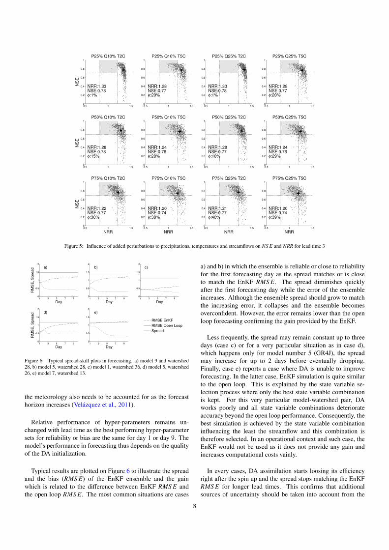
the meteorology also needs to be accounted for as the forecasthorizon increases (Velazquez et al., 2011).

Relative performance of hyper-parameters remains un-changed with lead time as the best performing hyper-parametersets for reliability or bias are the same for day 1 or day 9. Themodel’s performance in forecasting thus depends on the qualityof the DA initialization.

Typical results are plotted on Figure 6 to illustrate the spreadand the bias (RMS E) of the EnKF ensemble and the gainwhich is related to the difference between EnKF RMS E andthe open loop RMS E. The most common situations are cases

a) and b) in which the ensemble is reliable or close to reliabilityfor the first forecasting day as the spread matches or is closeto match the EnKF RMS E. The spread diminishes quicklyafter the first forecasting day while the error of the ensembleincreases. Although the ensemble spread should grow to matchthe increasing error, it collapses and the ensemble becomesoverconfident. However, the error remains lower than the openloop forecasting confirming the gain provided by the EnKF.

Less frequently, the spread may remain constant up to threedays (case c) or for a very particular situation as in case d),which happens only for model number 5 (GR4J), the spreadmay increase for up to 2 days before eventually dropping.Finally, case e) reports a case where DA is unable to improveforecasting. In the latter case, EnKF simulation is quite similarto the open loop. This is explained by the state variable se-lection process where only the best state variable combinationis kept. For this very particular model-watershed pair, DAworks poorly and all state variable combinations deteriorateaccuracy beyond the open loop performance. Consequently, thebest simulation is achieved by the state variable combinationinfluencing the least the streamflow and this combination istherefore selected. In an operational context and such case, theEnKF would not be used as it does not provide any gain andincreases computational costs vainly.

In every cases, DA assimilation starts loosing its efficiencyright after the spin up and the spread stops matching the EnKFRMS E for longer lead times. This confirms that additionalsources of uncertainty should be taken into account from the

8

1 2 3 4 5 6 7 8 9 101112

40

20

0

20

40

M1N

RR

NS

E

1 2 3 4 5 6 7 8 9 101112

40

20

0

20

40

M2

1 2 3 4 5 6 7 8 9 101112

40

20

0

20

40

M3

1 2 3 4 5 6 7 8 9 101112

40

20

0

20

40

M4

1 2 3 4 5 6 7 8 9 101112

40

20

0

20

40

M5

1 2 3 4 5 6 7 8 9 101112

40

20

0

20

40

M6

NR

RN

SE

1 2 3 4 5 6 7 8 9 101112

40

20

0

20

40

M7

1 2 3 4 5 6 7 8 9 101112

40

20

0

20

40

M8

1 2 3 4 5 6 7 8 9 101112

40

20

0

20

40

M9

1 2 3 4 5 6 7 8 9 101112

40

20

0

20

40

M10

1 2 3 4 5 6 7 8 9 101112

40

20

0

20

40

M11

NR

RN

SE

1 2 3 4 5 6 7 8 9 101112

40

20

0

20

40

M12

1 2 3 4 5 6 7 8 9 101112

40

20

0

20

40

M13

1 2 3 4 5 6 7 8 9 101112

40

20

0

20

40

M14

1 2 3 4 5 6 7 8 9 101112

40

20

0

20

40

M15

1 2 3 4 5 6 7 8 9 101112

40

20

0

20

40

M16

NR

RN

SE

1 2 3 4 5 6 7 8 9 101112

40

20

0

20

40

M17

1 2 3 4 5 6 7 8 9 101112

40

20

0

20

40

M18

Hyper−parameter sets

1 2 3 4 5 6 7 8 9 101112

40

20

0

20

40

M19

1 2 3 4 5 6 7 8 9 101112

40

20

0

20

40

M20

Figure 7: Frequency at which each of the 12 sets of hyper-parameters is better than others in term of accuracy (NS E) and reliability (NRR). Each boxplotcorresponds to a model (see Table 1) and results are displayed for lead time 3

first forecasting day to achieve a reliable system and alsoimplies that finding the best hyper-parameters only guaranteesto find the optimal initialization without ensuring forecastingperformances.

To investigate the possible relation between models andhyper-parameters, Figure 7 shows the frequency at which ahyper-parameter set outperforms the other for a given model.Each of the 20 sub-plot corresponds to a model. The 12 hyper-parameters are referred to by numbers as following:

1: P25%Q10%T2oC 2: P25%Q10%T5oC 3: P25%Q25%T2oC4: P25%Q25%T5oC 5: P50%Q10%T2oC 6: P50%Q10%T5oC7: P50%Q25%T2oC 8: P50%Q25%T5oC 9: P75%Q10%T2oC

10: P75%Q10%T5oC 11: P75%Q25%T2oC 12: P75%Q25%T5oC

The bars represent the frequency at which a hyper-parameterset outperforms the other. The upper part and lower part ofthe figure refer to the bias and reliability respectively. Forinstance, the hyper-parameter set number 10 is the best one forapproximatively 10% of the catchments for the bias and 35%for reliability for the model 1.

The repartition of the best performing hyper-parametersconfirms that no hyper-parameter set performs better thanothers systematically for the NS E or the NRR and exceedsrarely 40% for any model. Thus, to ensure to get optimalupdating performance, an optimal hyper-parameter should bechosen according to model and catchment.

An additional difficulty arises from the fact that bias andreliability are optimized by different hyper-parameters. Op-timal NS E values are often obtained by low to moderatenoise magnitude while the best NRR are obtained with higher

perturbations. This highlights the challenge to optimizebias and reliability collectively during EnKF updating, leav-ing to the modeller the burden of prioritizing one over the other.

3.3. Influence of the choice of states variables

For the the present section, results are shown for a particularhyper-parameters set P 50% Q 10% T 5% but similar conclu-sions could be drawn from the other tested sets.

This section addresses the question of identification ofstate variables that should be updated with the EnKF. Fora N-state-variable-model, it exists 2N − 1 combinations andnone is favored during testing. Thus, the number of possibil-ities depends on the model; see Table 1 for the number of states.

As the reservoirs are situated at different levels in the models(from interception to routing), their individual updating isexpected to affect differently model outputs; more preciselythey affect the time-lag between state perturbation and thechange in simulated streamflow. Seo et al. (2003) suggest to notperturb reservoirs concerning soil moisture as it is a long-termcomponent that has an influence which lasts much longer thanthe longest operationally used lead time. On the contrary,Wohling et al. (2006) encourage soil moisture updating as itwill act on all lead times. Physically based models offer thepossibility to deal with values that are theoretically measurable.The knowledge about these values allows to estimate criticalvalues that are the most subject to uncertainty. Conceptualmodels states values do not refer directly to a measurable valueand the identification of variable states for updating is thuscomplex. The amount of uncertainty related to these variablesis hardly definable and there is no apparent clue to update a

9

0

0.5

1

Da

y1

0

0.5

1

NS

E

Da

y3

0

0.5

1

Da

y6

M02 M05 M08

Updated state variables

M13 M20

Figure 8: Distribution of NS E performance over the 38 catchments for model 2, 5, 8, 13, and 20 according to the updated states parameters for lead time 1, 3, and6. The boxplot on the right of each sub-plot corresponds to the case where all states variable are updated.

certain reservoir and leaving others unperturbed.

Figure 8 presents the distribution of performance of everyindividual state combination per model, to illustrate thevariability of NS E over the 38 catchments. Five modelswith different numbers of state variable are used to highlightthe general 20 models behavior. Each box plot refers to acombination of updated state variable for a model. The boxplot situated on the right of each sub-plot corresponds to thecase where all model states are updated.

The main conclusion is twofold: the success of the updatingprocedure lays as much in the model as in the choice of thestate variables. Most models best state combinations exhibit amedian NS E higher than 0.75 for first lead time even if fewmodels (model 2 in particular) seem to react poorly to the stateupdating. Best short-lead-time-model performance needs tobe qualified as it frequently decreases with increasing lead time.

As median NS E values are frequently close to each other, itis possible to conclude that there is no obvious outperformingcombination for any model – however, there are combinationsthat perform consistently poorly. Additional complexity inthe choice of the best state combination to update arises fromthe performance variability over catchments for a specificupdated set of states. As the median performance is closeand the variability over catchments is important, it is verylikely that one combination for a model on a catchment willbe outperformed by another combination on another catchment.

As the state updating procedure is numerically implementedin the same way for all models, bad performance may beattributed to the suboptimal choice of updated model states orthe potential inadequacy of the EnKF to a specific hydrologicmodel rather than the EnKF technique itself. On this subject,model number 2 open loop performances are often comparablewith other models (see also Fig. 2) while its performance after

updating are undoubtedly worse.

The question of best state set identification arises also as afunction of the lead times (results not shown). In this study,we disregarded lead time specific states combinations since theuse of different set of state combinations lead time dependantmay improve performance for each lead time in average but itwould imply to run in a parallel fashion several simulations foreach lead time. An issue arising from such a technique wouldbe the creation of discontinuities in the forecasting streamflowsfrom one lead time to another.

Reservoirs which should be updated in priority are fre-quently –but not always– the closest reservoirs to the modeloutputs in the description of the rainfall-runoff process. Thequestion of the number of reservoir to update is more complexas few global patterns emerge from the results. It is commonpractice to update all model states variable but this does notsystematically lead to the best results (see also McMillan et al.,2013; Rakovec et al., 2015). In Fig 8, model 13 illustrates thissince the updating of some state variable sub-ensembles showsimproved performance for first, second and third quartiles.Therefore, for some models, optimal updating may be obtainedby leaving some stores from the update, for instance the routingstore for model 13. Generally, the number of updated statesremain rather low, never exceeding 4 even for high dimensionalstates models (model 7, 12 and 14). All states should beupdated for model 5, 6, 10 and 19 but other models statesshould be partially updated. Models with a large number ofstate variable (high degree of freedom) are more prone to en-counter equifinality issues as many outcomes frequently end upclose for a specific conditions. This lead to an already knownproblem that requires the user to take an arbitrary decisionor possibly to retain several combination with the associatedcomputational cost increase. Also, likewise for traditionalmodel parameter estimation, the identification of best setdepend on the score used as objective function. Selecting states

10

−0.5

0

0.5

1

Day1

Global updating − open loop gain

−0.5

0

0.5

1

Local updating − open loop gain

−0.5

0

0.5

1

Local − global updating gain

−0.5

0

0.5

1

NS

E g

ain

Day3

−0.5

0

0.5

1

−0.5

0

0.5

1

−0.5

0

0.5

1

M05 M10 M15 M20

Day6

−0.5

0

0.5

1

M05 M10 M15 M20−0.5

0

0.5

1

M05 M10 M15 M20

Figure 9: EnKF - open loop gains in NS E gains over the 38 catchments for global and locally defined hyper-parameters and state variable for lead time 1, 3 and 6.

set based on a NS E criterion does not guarantee to maximizeother accuracy scores, and even less to achieve highest possiblereliability. Thus, different sets of updated states may capturemore or less accurately specificities of the hydrograph.

3.4. Global and local updating schemes

Setting EnKF catchment specificities is possible and maybe operationally conceivable and worth considering. This caseis more computationally demanding as states identificationneeds to be carried out for all watersheds. Thus, the gain ofsuch approach needs to be quantified to justify the increase incommitment. In the opposite case, the forecaster takes a riskrelying on optimal updated states set identified from only onecatchment if this set is transferred onto another catchment.

Figure 9 displays gains obtained by EnKF over open loop.Two EnKF updating schemes are compared:

• A global scheme: updating is carried out with a single setof state variables and hyper-parameter per model, identi-fied as best according to the combined criterion in averageover all catchments. The updated states and the hyper-parameters are the same regardless of catchment.

• A local scheme : updating is carried out with a differentset of state variables and set of hyper-parameters for eachcatchment identified as the best set of state variable percatchment. The approach is thus catchment specific.

The gain between the two updating schemes is also ex-amined. In that case, the global performance is used as thereference in the gain equation (Eq. 11).

Overall, both EnKF schemes enhance open loop forecastsin the vast majority of cases, from short to longer lead time.

−0.5

0

0.5

1

Day1

Local − global updating gain

−0.5

0

0.5

1

Day3

NR

R g

ain

−0.5

0

0.5

1

M05 M10 M15 M20

Day6

Figure 10: EnKF-open loop gains in NRR over the 38 catchments for globaland locally defined hyper-parameters and state variable for lead time 1, 3 and 6

However, the gain in accuracy depends heavily on modeland to a lesser extent on the global-local updating scheme.One can notice that models 2, 13 and 20 have a structurethat react poorly to EnKF updating, especially for globalstates updating. The increase of computational resourcesmay not be worth the potential gain in performance forthe majority of catchments. Yet, these results are improvedin the case where catchment specific state variable sets are used.

It is frequent –and normal– that the differences betweenthe two updating schemes global/local for the same modelare small. This is the case when a model has frequently thesame best set of state variable over the 38 catchments whichtherefore turns to be the best in average over catchmentsand explains the frequent small dispersion of the local/globalupdating gain. However extremes are high as they are obtained

11

−0.5

0

0.5

1

Day1

Global updating − open loop gain

−0.5

0

0.5

1

Local updating − open loop gain

−0.5

0

0.5

1

Local − global updating gain

−0.5

0

0.5

1

NS

E g

ain

Day3

−0.5

0

0.5

1

−0.5

0

0.5

1

5 10 15 20 25 30 35−0.5

0

0.5

1

Day6

Catchments

5 10 15 20 25 30 35−0.5

0

0.5

1

Catchments

5 10 15 20 25 30 35−0.5

0

0.5

1

Catchments

Figure 11: EnKF - open loop gains in NS E over the 20 models for global and locally defined hyper-parameters and state variable for lead time 1, 3 and 6 accordingto catchments

when the global updating fails largely on a catchment. Thelocal scheme is logically better than global as it is designed toperform on all catchments but this does not ensure to be betterthan the global scheme in all cases. Indeed, even if the localupdating is catchment specific, it is still averaged on lead timesand thus the global state variable set may perform better for aparticular lead time.

Figure 10 represents the gain between the local and theglobal updating procedure in reliability (no comparison ispossible with the open loop as it is a deterministic forecast).The gain in reliability is consistently high for the first leadtime as the second quartile is always positive and third quantilehigher than 0.8 for most of the models. Some models, as themodel 9, 12, 14 should be preferentially updated in a local waybecause their gain is substantial (third quartile is greater than0.95). Interestingly, these models are among the most complexones in the model pool and seem to require a more detailedsetting to exploit optimally the EnKF for the first lead time. Aswith the NS E, the NRR gain decreases with lead time but staysmostly positive up to day 6 (see also Fig. 6). The gain may benegative for the reasons aforementioned with the NS E.

3.5. Influence of the catchments

To assess the importance of the catchments on forecastingperformance, Figure 11 represents the models’ NS E over the38 watersheds. This complementary vision of Figure 9 revealsthat catchments also have an influence on simulations that is asimportant as hyper-parameters, model structure, and the statevariable selection.

The majority of the catchment can benefit from EnKFupdating, especially in the case where local updating is used.Yet, there is a disparity in the gain as few catchments display anegative median gain, namely catchments 4, 8, 9, 10, 11, and12 for the first lead time and global updating and catchments 9and 11 for local updating.

The gain diminishes with increasing lead time except forthe catchments that exhibit a negative gain from day one. Theunderlying reason is that EnKF is not able to update correctlythe state variables, attributing erroneous values to the statevariable, combined with the fact that the updated state variableshave a greater influence for short lead times.

EnKF performance and gain were compared to the availableclimatic data and catchments characteristics. Specifically, theaverage annual total and liquid precipitation, the area and theestimated concentration time were put under scrutiny. No clearcorrelation between these values and EnKF performance hasbeen identified.

4. Conclusion and recommendations

This paper discusses the performance and implementationof EnKF in forecasting over a wide variety of catchmentsand rainfall-runoff lumped models. An extensive testing wascarried out to assess EnKF state updating and how it relates tomodel, catchment, and lead times.

The results show that an optimal implementation of theEnKF is more complex than frequently suggested and that a

12

detailed attention should be paid to the specification of hyper-parameters and updated state variable. While identification ofthe minimal number of members is relatively straightforwardas a vast majority of models and catchment agree, there is nosingle and universal optimal EnKF implementation for anymodel. In practice, it is unlikely that the best state combi-nation and hyper-parameter set in average are optimal for allwatersheds. Unlike many case studies, it is not reasonableto recommend precise values, as the best EnKF settings arefrequently case specific.

The hyper-parameters and more specifically, the perturba-tions of the inputs are frequently unintuitive to identify asthere are often unrealistically high to implicitly account forother sources of uncertainty, especially parameter and struc-tural uncertainty, and to eventually ensure model simulationreliability. An additional challenge arises from the difficultyto optimize reliability and ensemble median bias jointly as theimprovement of one criterion is achieved at the expense of theother.

Models encounter important differences in their results andin the way they should be updated. Models with a high numberof state variable (high degree of freedom) should receivean increased attention as they are more prone to encounterequifinality issues as many outcomes frequently end up closefor a specific condition.

Regardless of the model, ensemble reliability decreasesquickly with lead time as the ensemble spread drops from firstdays while the bias increases. This also underlines that takinginto account explicitly initial condition uncertainty solely is notsufficient for medium range forecasting and that structural errorand forcing error are dominant in modelling rainfall-runoff

processes.

Despite these constrains, the gain that EnKF provides overopen loop is substantial, especially if the optimization iscarried out locally. The later implies a detailed testing of allcombination to identify best performing EnKF implementationbut is computationally more expensive. As the EnKF is notefficient with every model and catchment, we recommend toinvestigate data assimilation coupling with several models togo beyond EnKF - model structure compatibility issue.

Finally, we encourage EnKF users to perform a detailedanalysis addressing the question of hyper-parameter and statevariable selection of their system to ensure to make the mostof EnKF. For further improvement, we also suggest to reportexplicitly the hyper-parameters and state variables they used tocontribute to a better understanding of EnKF parametrizationand to identify techniques that would allow to robustly identifythe pertinent state variables that should be updated without theneed to run all possible combinations.

5. Acknowledgements

The authors acknowledge the Centre d’Expertise Hydriquedu Quebec for providing hydrometeorological data. They alsoacknowledge financial support from the Chaire de rechercheEDS en previsions et actions hydrologiques and from the Natu-ral Sciences and Engineering Research Council of Canada.

References

Abaza, M., Anctil, F., Fortin, V., Turcotte, R., 2014. Sequential streamflowassimilation for short-term hydrological ensemble forecasting. J Hydrol 519,2692–2706.

Ajami, N. K., Duan, Q. Y., Sorooshian, Q., 2007. An integrated hydrologicBayesian multimodel combination framework: Confronting input, parame-ter, and model structural uncertainty in hydrologic prediction. Water ResourRes 43, 1–19.

Alvarez-Garreton, C., Ryu, D., Western, A. W., Crow, W. T.,Robertson, D. E.,2014. The impacts of assimilating satellite soil moisture into a rainfall-runoff

model in a semi-arid catchment. J Hydrol 519, 2763–2774.Andreadis, K.M., Lettenmaier, D.P., 2006. Assimilating remotely sensed snow

observations into a macroscale hydrology model. Adv Water Resour 29,872–886.

Bailey, R.T., Bau, D., 2012. Estimating geostatistical parameters and spatially-variable hydraulic conductivity within a catchment system using an ensem-ble smoother. Hydrol Earth Syst Sc 16, 287–304.

Bergstrom, S., Forsman, A., 1973. Development of a conceptual deterministicrainfall-runoff model. Nord Hydrol 4, 147–170.

Beven, K., Binley, A., 1992. The future of distributed models - model calibra-tion and uncertainty prediction. Hydrol Process 6, 279–298.

Beven, K.J., Kirkby, M.J., Schofield, N., Tagg, A.F., 1984. Testing a physically-based flood forecasting model (TOPMODEL) for 3 uk catchments. J Hydrol69, 119-143.

Burnash, R.J.C., Ferral, R.L., McGuire, R.A., 1973. A generalized streamflowsimulation system - Conceptual modelling for digital computers. US De-partment of Commerce, National Weather Service and State of California,United States, 204pp.

Chen, H., Yang, D.W., Hong, Y., Gourley, J.J., Zhang, Y., 2013. Hydrologicaldata assimilation with the ensemble square-root-filter: Use of streamflowobservations to update model states for real-time flash flood forecasting.Adv Water Resour 59, 209–220.

Chiew, F.H.S., Peel, M.C., Western, A.W., 2002. Application and testing of thesimple rainfall-runoff model SIMHYD, in Mathematical Models of SmallWatershed Hydrology and Applications. Water Resources Publication, Lit-tleton, Colorado, United States, 335–367.

Clark, M.P., Rupp, D.E., Woods, R.A., Zheng, X., Ibbitt, R.P., Slater, A.G.,Schmidt, J., Uddstrom, M.J., 2008. Hydrological data assimilation with theensemble kalman filter: Use of streamflow observations to update states in adistributed hydrological model. Adv Water Resour 31, 1309–1324.

Cormary, Y., Guilbot, A., . Etude des relations pluie-debit sur trois bassinsversants d’investigation, IAHS Madrid Symposium, IAHS Publication no.108, 265–279.

DeChant, C.M., Moradkhani, H., 2011. Improving the characterization of ini-tial condition for ensemble streamflow prediction using data assimilation.Hydrol Earth Syst Sc 15, 3399–3410.

DeChant, C.M., Moradkhani, H., 2012. Examining the effectiveness and ro-bustness of sequential data assimilation methods for quantification of uncer-tainty in hydrologic forecasting. Water Resour Res 48, 1–15.

Duan, Q.Y., Ajami, N.K., Gao, X.G., Sorooshian, S., 2007. Multi-model en-semble hydrologic prediction using bayesian model averaging. Adv WaterResour 30, 1371–1386.

Duan, Q.Y., Sorooshian, S., Gupta, V., 1992. Effective and efficient globaloptimization for conceptual rainfall-runoff models. Water Resour Res 28,1015–1031.

Evensen, G., 1994. Sequential data assimilation with a nonlinear quasi-geostrophic model using monte-carlo methods to forecast error statistics.J Geophys Res-Oceans 99, 10143–10162.

Evensen, G., 2003. The ensemble kalman filter: theoretical formulation andpractical implementation. Ocean Dynam 53, 343–367.

13

Forman, B.A., Reichle, R.H., Rodell, M., 2012. Assimilation of terrestrial waterstorage from grace in a snow-dominated basin. Water Resour Res 48, 1–14.

Fortin, V., Abaza, M., Anctil, F., Turcotte, R., 2014. Why should ensemblespread match the rmse of the ensemble mean? J Hydrometeorol 15, 1708 –1713.

Franz, K. J., Hogue, T. S., Bank, M., He, M. X., 2014. Assessment of SWEdata assimilation for ensemble streamflow predictions. J Hydrol 519, 2737– 2746.

Fortin, V., Turcotte, R., 2007. Le modele hydrologique MOHYSE, Note decours pour SCA7420. Report. Departement des sciences de la terre et del’atmosphere, Universite du Quebec a Montreal, Canada, 17pp.

Garcon, R., 1999. Modele global pluie-debit pour la prevision et lapredetermination des crues. Houille Blanche 7/8, 88–95.

Girard, G., Morin, G., Charbonneau, R., 1972. Modele precipitations-debits adiscretisation spatiale. Cahiers ORSTOM, Serie Hydrologie 9, 35–52.

Harader, E., Borrell-Estupina, V., Ricci, S., Coustau, M., Thual, O., Piacentini,A., Bouvier, C., 2012. Correcting the radar rainfall forcing of a hydrologi-cal model with data assimilation: application to flood forecasting in the lezcatchment in southern france. Hydrol Earth Syst Sc 16, 4247–4264.

Hong, Y., Hsu, K. L., Moradkhani, H., Sorooshian, S., 2006. Uncertainty quan-tification of satellite precipitation estimation and Monte Carlo assessment ofthe error propagation into hydrologic response. Water Resour Res 42, 1–15.

Jakeman, A.J., Littlewood, I.G., Whitehead, P.G., 1990. Computation of theinstantaneous unit hydrograph and identifiable component flows with appli-cation to two small upland catchments. J Hydrol 117, 275–300.

Jeremiah, E., Sisson, S., Marshall, L., Mehrotra, R., Sharma, A., 2011.Bayesian calibration and uncertainty analysis of hydrological models: Acomparison of adaptive metropolis and sequential monte carlo samplers.Water Resour Res 47, 1–13.

Kim, J., Yoo, C., 2014. Use of a dual Kalman filter for real-time correction ofmean field bias of radar rain rate. J Hydrol 519, 2785–2796.

Kuchment, L.S., Romanov, P., Gelfan, A.N., Demidov, V.N., 2010. Use ofsatellite-derived data for characterization of snow cover and simulation ofsnowmelt runoff through a distributed physically based model of runoff gen-eration. Hydrol Earth Syst Sc 14, 339–350.

Kuczera, G., Kavetski, D., Franks, S., Thyer, M., 2006. Towards a Bayesian to-tal error analysis of conceptual rainfall-runoff models: Characterising modelerror using storm-dependent parameters. J Hydrol 331, 161–177.

Lee, H., Seo, D.J., Koren, V., 2011. Assimilation of streamflow and in situsoil moisture data into operational distributed hydrologic models: Effects ofuncertainties in the data and initial model soil moisture states. Adv WaterResour 34, 1597–1615.

Li, Y., Ryu, D., Western, A. W., Wang, Q. J., 2013. Assimilation of streamdischarge for flood forecasting: The benefits of accounting for routing timelags. Water Resour Res 49, 1887 – 1900.

Li, Y., Ryu, D., Western, A. W., Wang, Q. J., Robertson, D. E., Crow, W. T.,2014. An integrated error parameter estimation and lag-aware data assimi-lation scheme for real-time flood forecasting. J Hydrol 519, 2722 – 2736.

Liu, Y. Q., Gupta, H. V., 2007. Uncertainty in hydrologic modeling: Toward anintegrated data assimilation framework. Water Resour Res 43, 1 – 18.

Liu, Y., Weerts, A. H., Clark, M., Franssen, H. J. H., Kumar, S., Moradkhani,H., Seo, D. J., Schwanenberg, D., Smith, P., Van Dijk, A., Van Velzen, N.,He, M., Lee, H., Noh, S., Rakovec, O., Restrepo, P., 2012. Advancing dataassimilation in operational hydrologic forecasting: progresses, challenges,and emerging opportunities. Hydrol Earth Syst Sc 16, 3863 – 3887.

Mandel, J., 2006. Efficient Implementation of the Ensemble Kalman Filter.Report. UCDHSC, Denver, Colorado, United States. 9pp.

Mazenc, B., Sanchez, M., Thiery, D., 1984. Analyse de l’influence de la phys-iographie d’un bassin versant sur les parametres d’un modele hydrologiqueglobal et sur les debits caracteristiques a l’exutoire. J Hydrol 69, 97–188.

McMillan, H.K., Hreinsson, E.O., Clark, M.P., Singh, S.K., Zammit, C., Ud-dstrom, M.J., 2013. Operational hydrological data assimilation with therecursive ensemble kalman filter. Hydrol Earth Syst Sc 17, 21–38.

Meier, P., Froemelt, A., Kinzelbach, W., 2011. Hydrological real-time mod-elling in the zambezi river basin using satellite-based soil moisture and rain-fall data. Hydrol Earth Syst Sc 15, 999–1008.

Moore, R.J., Clarke, R.T., 1981. A distribution function approach to rainfallrunoff modeling. Water Resour Res 17, 1367–1382.

Moradkhani, H., Sorooshian, S., Gupta, H.V., Houser, P.R., 2005. Dual state-parameter estimation of hydrological models using ensemble kalman filter.Adv Water Resour 28, 135–147.

Moradkhani, H.,Hsu, K., Hong, Y., Sorooshian, S., 2006. Investigating theimpact of remotely sensed precipitation and hydrologic model uncertaintieson the ensemble streamflow forecasting. Geophys Res Lett 33, 1–5.

Murphy, J.M., 1988. The impact of ensemble forecasts on predictability. Q JRoy Meteor Soc 114, 463–493.

Naevdal, G., Johnsen, L. M., Aanonsen, S. I., Vefring, E. H., 2003. Reservoirmonitoring and continuous model updating using ensemble Kalman filter.SPE J 10, 66–74.

Nash, J. E., Sutcliffe, I., 1970. River flow forecasting through conceptual mod-els. Part 1 - A discussion of principles. J Hydrol 10, 282–290.

Nie, S., Zhu, J., Luo, Y., 2011. Simultaneous estimation of land surface schemestates and parameters using the ensemble kalman filter: identical twin ex-periments. Hydrol Earth Syst Sc 15, 2437–2457.

Nielsen, S.A., Hansen, E., 1973. Numerical simulation of the rainfall-runoff

process on a daily basis. Nord Hydrol 4, 171–190.O’Connell, P.E., Nash, J.E., Farrell, J.P., 1970. River flow forecasting through

conceptual models, part ii - the brosna catchment at ferbane. J Hydrol 10,317–329.

Oudin, L., Hervieu, F., Michel, C., Perrin, C., Andreassian, V., Anctil, F., Lou-magne, C., 2005. Which potential evapotranspiration input for a lumpedrainfall-runoff model? part 2 - towards a simple and efficient potential evap-otranspiration model for rainfall-runoff modelling. J Hydrol 303, 290–306.

Parrish, M. A., Moradkhani, H., Dechant, C., 2012. Toward reduction of modeluncertainty: Integration of Bayesian model averaging and data assimilation.Water Resour Res 48, 1–18.

Perrin, C., 2000. Vers une amelioration d’un modele global pluie-debit. Thesis.Institut National Polytechnique de Grenoble - INPG, France. 289pp.

Perrin, C., Michel, C., Andreassian, V., 2003. Improvement of a parsimoniousmodel for streamflow simulation. J Hydrol 279, 275–289.

Rakovec, O., Weerts, A.H., Hazenberg, P., Torfs, P., Uijlenhoet, R., 2012. Stateupdating of a distributed hydrological model with ensemble kalman filtering:effects of updating frequency and observation network density on forecastaccuracy. Hydrol Earth Syst Sc 16, 3435–3449.

Rakovec, O., Weerts, A.H., Sumihar, J., Uijlenhoet, R., 2015. Operationalaspects of asynchronous filtering for flood forecasting. Hydrol Earth SystSc 19, 2911–2924.

Ramos, M.H., Mathevet, T., Thielen, J., Pappenberger, F., 2010. Communi-cating uncertainty in hydro-meteorological forecasts: mission impossible?Meteorol Appl 17, 223–235.

Reichle, R. H., Walker, J. P., Koster, R. D., Houser, P. R., 2002. Extended versusensemble Kalman filtering for land data assimilation. J Hydrometeorol 3,728–740.

Renzullo, L. J., Van Dijk, A., Perraud, J. M., Collins, D., Henderson, B., Jin,H., Smith, A. B., McJannet, D. L., 2014. Continental satellite soil moisturedata assimilation improves root-zone moisture analysis for water resourcesassessment. J Hydrol 519, 2747–2762.

Salamon, P., Feyen, L., 2010. Disentangling uncertainties in distributed hy-drological modeling using multiplicative error models and sequential dataassimilation. Water Resour Res 46, 1–20.

Seiller, G., Anctil, F., Perrin, C., 2012. Multimodel evaluation of twenty lumpedhydrological models under contrasted climate conditions. Hydrol Earth SystSc 16, 1171–1189.

Seo, D.J., Cajina, L., Corby, R., Howieson, T., 2009. Automatic state updatingfor operational streamflow forecasting via variational data assimilation. JHydrol 367, 255–275.

Seo, D.J., Koren, V., Cajina, N., 2003. Real-time variational assimilation ofhydrologic and hydrometeorological data into operational hydrologic fore-casting. J Hydrometeorol 4, 627–641.

Sugawara, M., 1979. Automatic calibration of the tank model. Hydrolog Sci J24, 375–388.

Thiery, D., 1982. Utilisation d’un modele global pour identifier sur un niveaupiezometrique des influences multiples dues a diverses activites humaines.IAHS-AISH Publication 136, 71–77.

Thirel, G., Martin, E., Mahfouf, J.F., Massart, S., Ricci, S., Regimbeau, F., Ha-bets, F., 2010. A past discharge assimilation system for ensemble streamflowforecasts over france - part 2: Impact on the ensemble streamflow forecasts.Hydrol Earth Syst Sc 14, 1639–1653.

Thornthwaite, C.W., Mather, J.R., 1955. The water balance. Report. DrexelInstitute of Climatology, Centerton, New Jersey, United States, 1–104.

Valery, A., Andreassian, V., Perrin, C., 2014. ’As simple as possible but notsimpler’: What is useful in a temperature-based snow-accounting routine?

14

part 1 - comparison of six snow accounting routines on 380 catchments. JHydrol 517, 1166–1175.

Velazquez, J.A., Anctil, F., Ramos, M.H., Perrin, C., 2011. Can a multi-modelapproach improve hydrological ensemble forecasting? A study on 29 Frenchcatchments using 16 hydrological model structures. Adv Geosci 29, 33–42.

Vrugt, J.A., Diks, C.G.H., Gupta, H.V., Bouten, W., Verstraten, J.M., 2005.Improved treatment of uncertainty in hydrologic modeling: Combining thestrengths of global optimization and data assimilation. Water Resour Res41, 1–17.

Vrugt, J.A., Gupta, H.V., Bouten, W., Sorooshian, S., 2003. A shuffled complexevolution metropolis algorithm for optimization and uncertainty assessmentof hydrologic model parameters. Water Resour Res 39, 1–14.

Vrugt, J.A., Robinson, B.A., 2007. Treatment of uncertainty using ensemblemethods: Comparison of sequential data assimilation and bayesian modelaveraging. Water Resour Res 43, 1–15.

Vrugt, J.A., Gupta, H.V., Nuallain, B. O., 2006. Real-time data assimilation foroperational ensemble streamflow forecasting. J Hydrometeorol 7, 548–565.

Wagener, T., Boyle, D.P., Lees, M.J., Wheater, H.S., Gupta, H.V., Sorooshian,S., 2001. A framework for development and application of hydrologicalmodels. Hydrol Earth Syst Sc 5, 13–26.

Warmerdam, P.M., Kole, J., Chormanski, J., 1997. Modelling rainfall-runoff

processes in the hupselse beek research basin, in: IHP-V, Technical Docu-ments in Hydrology, 155–160.

Weerts, A.H., El Serafy, G.Y.H., 2006. Particle filtering and ensemble kalmanfiltering for state updating with hydrological conceptual rainfall-runoff mod-els. Water Resources Research 42, 17.

Whitaker, J.S., Hamill, T.M., 2002. Ensemble data assimilation without per-turbed observations. Mon Weather Rev 130, 1913–1924.

Wohling, T., Lennartz, F., Zappa, M., 2006. Technical note: Updating proce-dure for flood forecasting with conceptual hbv-type models. Hydrol EarthSyst Sc 10, 783–788.

Zhao, R.J., Zuang, Y.L., Fang, L.R., Liu, X.R., Zhang, Q., 1980. The xinanjiangmodel. IAHS-AISH Publication 129, 351–356.

15