On the Dynamics of Price Discovery: Energy and

Agricultural Markets with and without the Renewable Fuels

Mandate

Layla Shiva, David A. Bessler, Bruce A. McCarl1

Selected Paper prepared for presentation at the Agricultural & Applied

Economics Association’s

2014 AAEA Annual Meeting, Minneapolis, MN, July 27-29, 2014.

Copyright 2014 by Layla Shiva, David Bessler, Bruce McCarl. All rights reserved.

Readers may make verbatim copies of this document for non-commercial purposes by any

means, provided that this copyright notice appears on all such copies.

1 Layla Shiva is a PhD student, David A. Bessler is regent professor, and Bruce A. McCarl is regent

professor, all in department of Agricultural Economics, Texas A&M University. Correspondence can be

directed to: laylashiva@tamu.edu.

2

On the Dynamics of Price Discovery: Energy and

Agricultural Markets with and without the Renewable Fuels

Mandate

We model the energy–agriculture linkage through structural vector autoregression (VAR)

model. This model quantifies the relative importance of various contributing factors in

driving prices in both markets. The LiNGAM algorithm from the machine learning

literature is used to help identify structural parameters in contemporaneous time. We

perform conditional forecasting, taking into account the renewable fuel standards

policies, and compare the forecasted path of prices with and without the renewable fuels

mandates.

Key Words: ethanol, vector autoregression, renewable fuel standard, graph theory

Introduction

Enhancing energy security and GHG emission reduction are important reasons to

promote renewable energy sources such as biofuels. To encourage biofuels, US

government has implemented ethanol subsidies and renewable fuel standards on the

amount of ethanol to be blended to transportation fuel. Ethanol is a gasoline additive.

Since it contains higher octane than gasoline, it burns cleaner. The feedstock for grain

ethanol (or first generation of biofuels) is mainly corn. The increase in corn demand as a

biofeedstocks, especially after 2006 ethanol boom, and limited land resources causes a

competition for land between food and fuel. Accordingly, a strong link between crude

3

oil, gasoline and corn prices has been formed. The evolving interdependency between

energy and agriculture markets in US is the subject of this study.

Subsidization of ethanol in the United States began with the Energy Policy Act of

1978. Since then, the subsidy has ranged between 40¢ per gallon and 60¢ per gallon of

ethanol, and until it was discontinued on December 31, 2011 was 45¢ per gallon (Abbott,

Hurt and Tyner 2011). Throughout the last three decades of ethanol production, the

subsidy has been a fixed amount, invariant with oil or corn prices (Tyner and Taheripour

2008). In 1990, the Clean Air Act was passed, which required vendors of gasoline to

have a minimum oxygen percentage in their product because adding oxygen enables the

fuel to burn cleaner. Therefore a cleaner environment became another important reason

for ethanol subsidies.

For the oil industry to meet the oxygen percentage standard requirements, there were

two options: 1) use ethanol that contains a high percentage of oxygen by weight, or 2) use

methyl tertiary butyl ether (MTBE). MTBE was generally a cheaper alternative than

ethanol, so it was the favored way of meeting the oxygen requirements throughout the

1990s. However MTBE showed negative environmental consequences infiltrating water

supplies and it was viewed as highly toxic. Consequently, MTBE was gradually banned

on a state-by-state basis (Birur, Hertel and Tyner 2009).

The 2006 Ban of MTBE, combined with high crude oil price (which climbed to over

$100/bbl in 2004) and the ethanol tax credit raised the profitability of ethanol industry

particularly beginning in 2004 and 2005. High profit margins from ethanol production in

2004–2007 encouraged a rapid investment in ethanol industry in these years (Tyner et al.

4

2008). Between 2006 and 2008, the correlation between crude oil and corn prices was

strong, in part because ethanol was needed to supply the oxygenate market. After 2008

the oxygenate market was largely saturated, ethanol prices ceased their rapid rise (and

corn prices rose significantly), making ethanol production unprofitable in many cases. In

2008-09 and afterward, we see a high correlation (about 0.84 in 2008) between ethanol

and corn prices, since the profitability of ethanol production depends on corn price

(Abbott, Hurt and Tyner 2011).

On December, 2007, the Energy Independence and Security Act of 2007 (H.R. 6) was

signed into law. This comprehensive energy legislation amends the Renewable Fuels

Standard (RFS) signed into law in 2005. RFS sets forth a phase-in for renewable fuel

volumes beginning with 9 billion gallons in 2008 and ending at 36 billion gallons in

2022. By doing so, the legislation seizes on the potential that renewable fuels offer an

opportunity to reduce foreign oil dependence and greenhouse gas emissions and provide

meaningful economic opportunity across this country; putting America firmly on a path

toward greater energy stability and sustainability (Renewable Fuel Association ).

Growth of the ethanol industry in last few years makes corn an energy crop, as well as

the world’s most important source of grain for production of livestock, poultry, and dairy

products. This transition established a relationship between ethanol and corn price and

also the products from corn. Production of biofuels affects the agriculture market in that

diversion of land to produce biofeedstocks may reduce the supply of other products and

as a result there is a likely rise in prices. Since ethanol is oxygen enhancing additive and

a replacement for gasoline, its price has a relationship with gasoline and also crude oil.

5

The ranges of fluctuation in these relationships have been different during past years

(Wisner 2009).

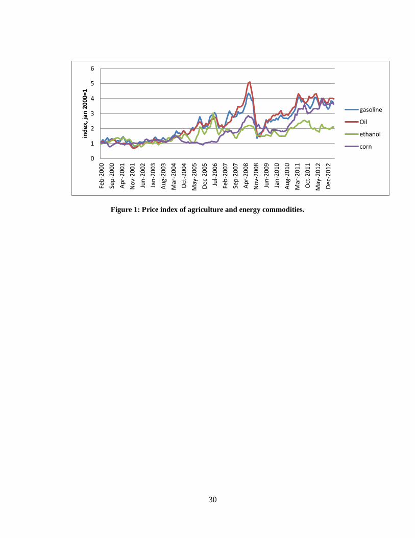
Figure 1 shows the indices of corn, crude oil, ethanol, and gasoline prices since 2000

based on data from energy information administration (EIA) and USDA. The main point

of this graph is commodity prices have moved together for the most part. As we can see

before 2007 corn price and crude oil price show small responses to each other’s

movement, but after this time they show a stronger relationship. The same is true for corn

and gasoline. Gasoline’s price has not increased as much as crude oil’s price since 2007,

the reason could be that crude oil is not the only cost factor in gasoline production.

In recent years, drop in gasoline usage in US and market limitations to future growth

in the blending of biofuel have resulted in fall of ethanol consumption (Westcott and

McPhail 2013). This fall even leads to unsatisfaction of RFS requirements and that cause

some uncertainty on EPA implementation of RFS for 2014 and beyond and penalties to

parties who are not able to encounter the requirements (Westcott and McPhail 2013).

Brief literature review

Birur, Hertel and Tyner (2009) examined the effect of the ethanol boom on the price

of other agricultural commodities. They indicated that the rapid growth of corn price in

2006-07 affected the price of soybeans as well, since there were substantial shifts of

soybeans acreage to corn. Corn is used primarily as an animal feed. Poultry, meat and

eggs faced largest shock as two-thirds of poultry feed consists of corn. As a consequence,

the total cost of producing poultry meat and eggs has increased by about 15 percent over

this period. Alexander and Hurt (2007) suggest that in the long run, food will be able to

6

compete successfully with the use of crops for fuel, but probably with somewhat higher

food prices and greater costs of food to consumers.

The literature does address the interactions of ethanol production and the energy

market. For instance, Du and Hayes (2009) calculated the average impact of ethanol

production on the gasoline price. Estimation results indicate that, on average, over the

whole sample period (2000-2010) the growth in ethanol production reduced wholesale

gasoline prices by $0.25/gallon. Also changes in the price of crude oil were found to have

effects on the biofuel’s production and prices. The FAO 2010 explains when crude oil

prices increase; two main factors affect agricultural commodity markets. First, the

production costs for the crop increase so this leads to a reduction in supply and therefore

raises commodity prices. Second, the increase in oil-based fuel prices provides an

incentive to biofuel producers to expand production, which in turn expands demand for

agricultural feedstock crops causing prices to increase more. The expansion in biofuel

supply may also decreases because of the rise in commodity prices. The net impact on

commodity markets will depend on the degree of increase in biofuel prices relative to the

increase in total crop production cost.

Bryant and Outlaw (2006) also studied the effect of absence, existence and different

combinations of government policies (RFS and exemption of tax credits) on ethanol

production and price by 2012. They conclude that due to powerful market-based

incentives the increases in levels of ethanol production would be likely in coming years,

even in the absence of government programs. Carter, Rausser and Smith (2012) also

estimate that corn prices were about 30 percent greater, on average, between 2006 and

7

2010 than they would have been if ethanol production had remained at 2005 levels with

no RFS. Tyner (2010) studied links between agriculture and energy markets and found

strong correlation between crude oil and corn prices in 2006-2008 and little link between

ethanol and corn prices. But in 2009, when there was ethanol surplus in the market the

link between ethanol and corn price was strongest.

Empirical methods

Vector Autoregression model

In this study, we use Vector autoregression (VAR) model for our analysis.

Considering regularities of world without imposing any prior restriction is an advantage

of VAR (Greene 2003). A VAR can be expressed as:

Where a (mx1) vector of variables and m is is the number of series. is a (qx1)

vector of strictly exogenous variables. and C are appropriately dimensioned matrices

of coefficients. The integers k and t are the number of lags and time indexes, respectively.

is the innovation term and it is assumed to be white noise, means E ( ) = 0.. The

innovations and are independent for s≠t. Although serially uncorrelated,

contemporaneous correlation among the elements of is possible, ∑= E is an

(mxm) positive definite matrix.

Contemporaneously correlated innovations could mislead the information one gleans

from the vector autoregression (by confounding innovation accounting results). A

Choleski factorization is one way to address this issue. In this method, we need to pre

multiply the system by lower triangular matrix , such that ∑ . The

8

problem with this method is that it imposes an ordering through Choleski factorization.

Our theory is sometimes not rich enough to suggest which series are exogenous. A

Bernanke factorization is another option which allows more general causal flows.

Following (Bernanke 1986) one can write the innovations as a linear function of

orthogonal innovations:

Multiplying matrix A to non-orthogonal innovations, gives orthogonal innovations

provides the identified structural VAR. The transformed VAR will thus look as follows:

If and = , then we can also write the equation in moving average form

as follows:

There exist some rules in the literature on number of free parameters to maintain

identification (Doan 1993). Compare to Choleski decomposition which imposed a just

identified structure, Bernanke allows more flexible identification method based on

theory. In this study we will use algorithms of inductive causation (Pearl 2000) with

acyclic graphical representations to hold identifying restrictions on matrix A (Awokuse

and Bessler 2003).

Directed Acyclic Graphs

The graphical approach to recognize the causal ordering among the variables is

directed acyclic graphs which is based on graph theory. This method pictures the causal

9

flow among the variables by using arrows and vertices (Pearl 2000) and statistically

inferred information about the probability distribution of the estimated residuals. In

another word, it consists of a set of variables and the directed or undirected edges

between some of the variables (Pearl 1995). A causal model such as A → B is a directed

graph, which means A causes B. It means one can change the value of B by changing the

value of A. A directed acyclic graph is a directed graph that contains no directed cyclic

paths (Spirtes, Glymour and Scheines 2000). For instance A→B→C→A is a cyclic

graph, since we return to the same variable as we start with.

Directed acyclic graphs show the conditional independencies as implied by the

recursive product decomposition (Awokuse and Bessler 2003):

Here Pr is the probability of the variables and is the minimum

subset of variables that comes before in causal sense.

Pearl (1995) also suggests the concept of D-separation as a method in DAGS to verify

the causal ordering. A variable d-separates two variable when it blocks the information

flow between them. One basic pattern of causal relationship is the causal chain

(A→B→C). In this chain A and C are dependent unless we condition on B. The other

pattern is causal fork (A← B→C), in which A and C are dependent until we condition on

B. Also the last pattern is a causal collider (A→B←C), in this case A and C are

independent but are dependent when we condition on B. DAGs realize the causal

direction first by testing the correlation between the variables and then by conditional

correlation on the third variables and following the above rules of causal ordering.

10

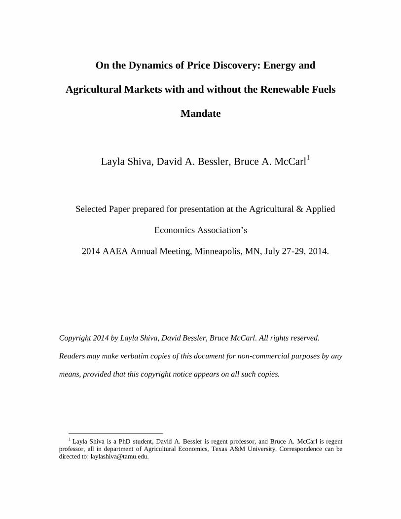
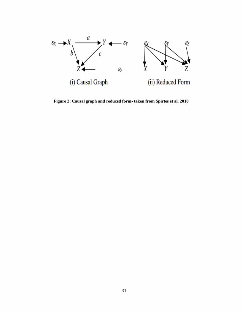
Figure 2 depicted the Lingam (Linear Non-Gaussian Acyclic Model) algorithm

(Shimizu et al. 2006) which is used in this study to figure out the causal ordering among

the variables. This method is appropriate when at most one of the variable’s noises may

be Gaussian. Spirtes et al. (2010) explain this method as a system such as:

1)

2)

3)

Where a, b and c are the coefficients and , , are independent noises. If we

write these equations in reduced forms, we will have:

4)

5)

6)

LiNGAM algorithm can find the correct matching of coefficients in the Independent

Component Analysis (ICA) matrix (Hyvärinen and Oja 2000) and prune away any

insignificant coefficients using statistical criteria (Spirtes et al. 2010). A unique DAG will

be constructed, since the coefficients are determined for each variable. The required

assumptions are: 1) no unmeasured common causes; 2) dependent variable could be

explained by a linear equation; 3) relation among variables are not deterministic; 4) i.i.d

sampling; 5) Markov condition, which is probability distribution explain one variable is

only condition on the variables of direct cause (Spirtes et al. 2010).

11

Forecasting and conditional forecasting

In the literature, using conditional forecasting is an approach to evaluate a policy. It is

of interest sometimes to consider the forecast of some variables in the system conditional

on some knowledge of the future path of other variables in the system. (Sims, Goldfeld

and Sachs (1982) address important issues on how to conduct a formal policy analysis.

We can use Vector Autoregression to do policy analysis. Assuming a policy

instrument is exogenous; one can view a VAR model’s forecasts conditional on different

hypothetical values of instrument as capturing the effect of alternative instrument settings

on the endogenous variables (Cooley and LeRoy 1985). If we force some values on

future path of one variable, this will result in restrictions on the other variables of the

system as well. In general forecasting our best guess of future disturbances could be zero,

but in conditional forecasting by forcing a value on some variables we cannot assume

zero disturbances on other variables. The disturbance is not zero to adapt real values to

the required (policy) values.

If we wish to forecast one period ahead conditional on a specific policy, we know the

future of policy variable and also the model at the current time. Here is the setup:

This equation is shows at time t we are predicting for t+1. Since we know the current

and past states (history), so we will have:

Identification of this system depends on the structure imbedded in the matrix . This

structure on , will communicate the implied path on other variables, in addition to the

12

policy variable whoes future values the governmental authority sets. Therefore for this

model to be identified, we need sufficient restrictions on matrix. For VAR in N

variables if we leave more than N(N-1)/2 parameters free (to be estimated) the model is

not identified. The restrictions on , come from theory or inductive causation. We can

use the algorithms of inductive causation (communicated through the DAG structure) on

the VAR innovations derive the restriction on in contemporaneous time.

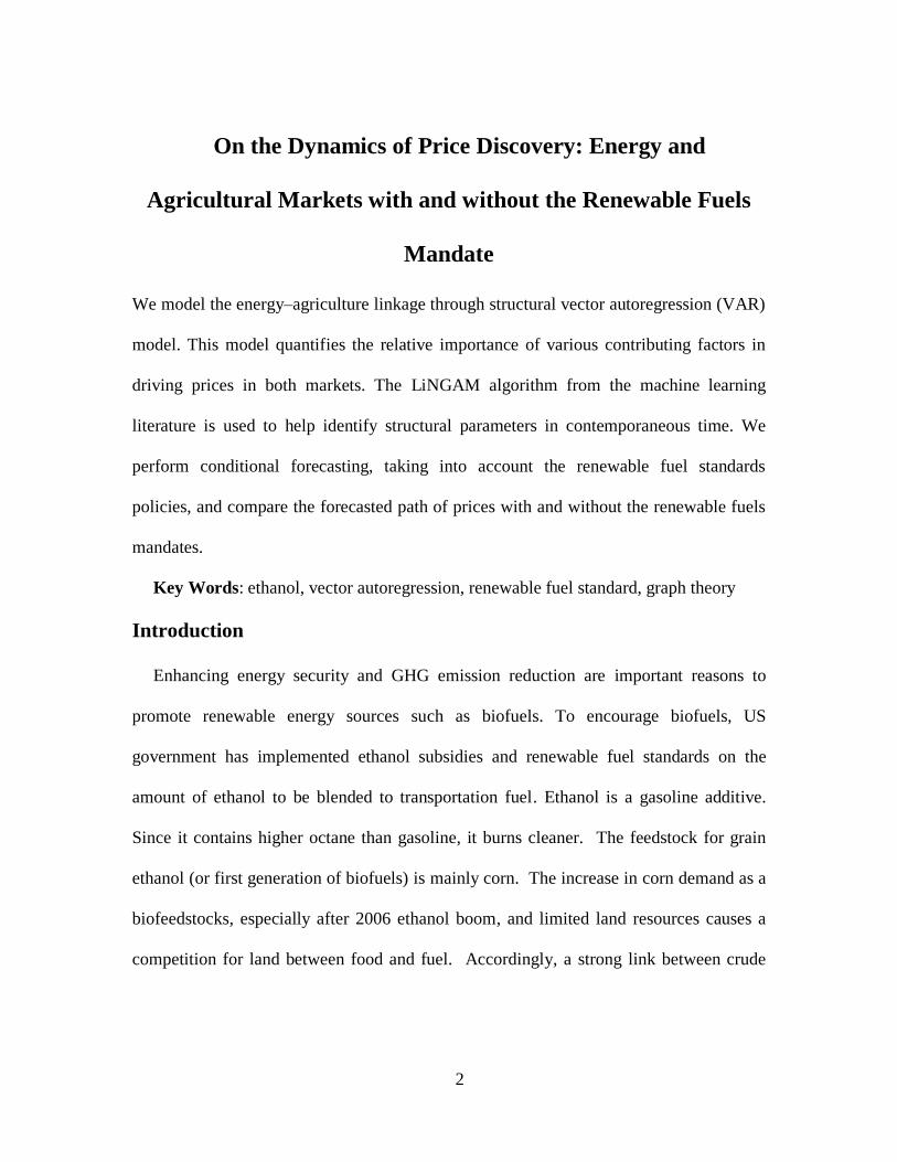
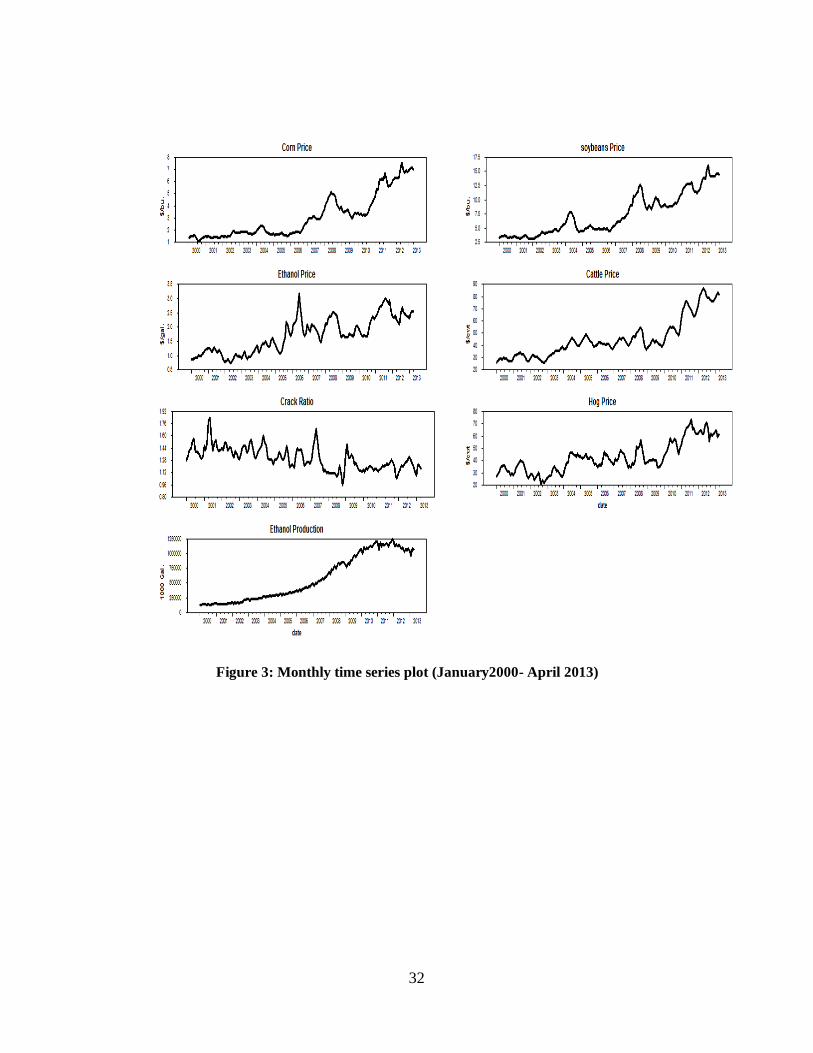
Data

The data of this study are monthly data, starting from January 2000 to April 2013 for

total observations of 160. We decide to choose data generated after 2000, since most

ethanol production increases over the post 2000 period. Our data includes corn price,

ethanol price (ethp), ethanol production (eprod) and also soybean price, cattle price and

hog price (soyp, cattp, hogp) are representatives to show the effects on agricultural

market. In addition we study the Crack ratio (crkr), to show effects of energy market

following Du and Hayes (2009) and Knittel and Smith (2012). The crack ratio is a

measure of the refining margin. Du and Hayes (2009) define it as the price of gasoline

divided by the price of oil. The gasoline price variable is the “total gasoline

wholesale/resale price by refiners”, which excludes taxes and reflects primarily gasoline

prior to blending with ethanol. The crude oil price is the “national average refiner

acquisition cost of crude oil”. These data and also Ethanol production are obtained from

the U.S. Energy Information Administration (EIA) website. The agricultural products

prices are from the USDA website. The ethanol price data source is Hart's Oxy-Fuel

News. The Data are deflated by the consumer price index (CPI). To get the real prices,

13

each price is divided by, CPI in each month/CPI in April 2013. CPI index is from U.S.

Bureau of Labor Statistics website. Plots of the price series for each market are provided

in Figure 3.

Empirical results

Stationarity

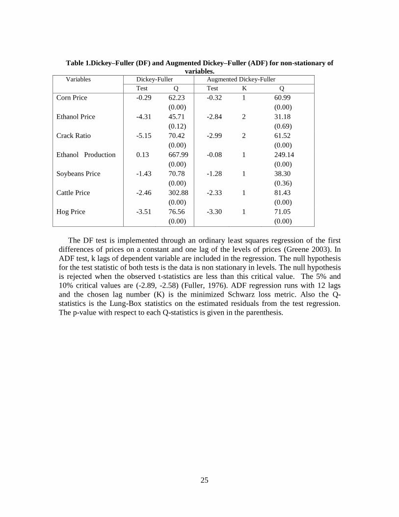
We have performed two test of stationarity of the variables, Dickey–Fuller (DF) and

Augmented Dickey–Fuller (ADF). DF and ADF test results are given in Table 1. DF

results show that at both critical value ethanol price, crack ratio and hog price are

stationary and the rest of variables are non-stationary. The ADF test also presents that the

crack ratio and hog price variables with 2 and 1 lag respectively, are stationary at 5%

critical value and at 10% critical value, ethanol price with 2 lags is also stationary. The

rest of variables are showing non stationary.

Optimal lag length

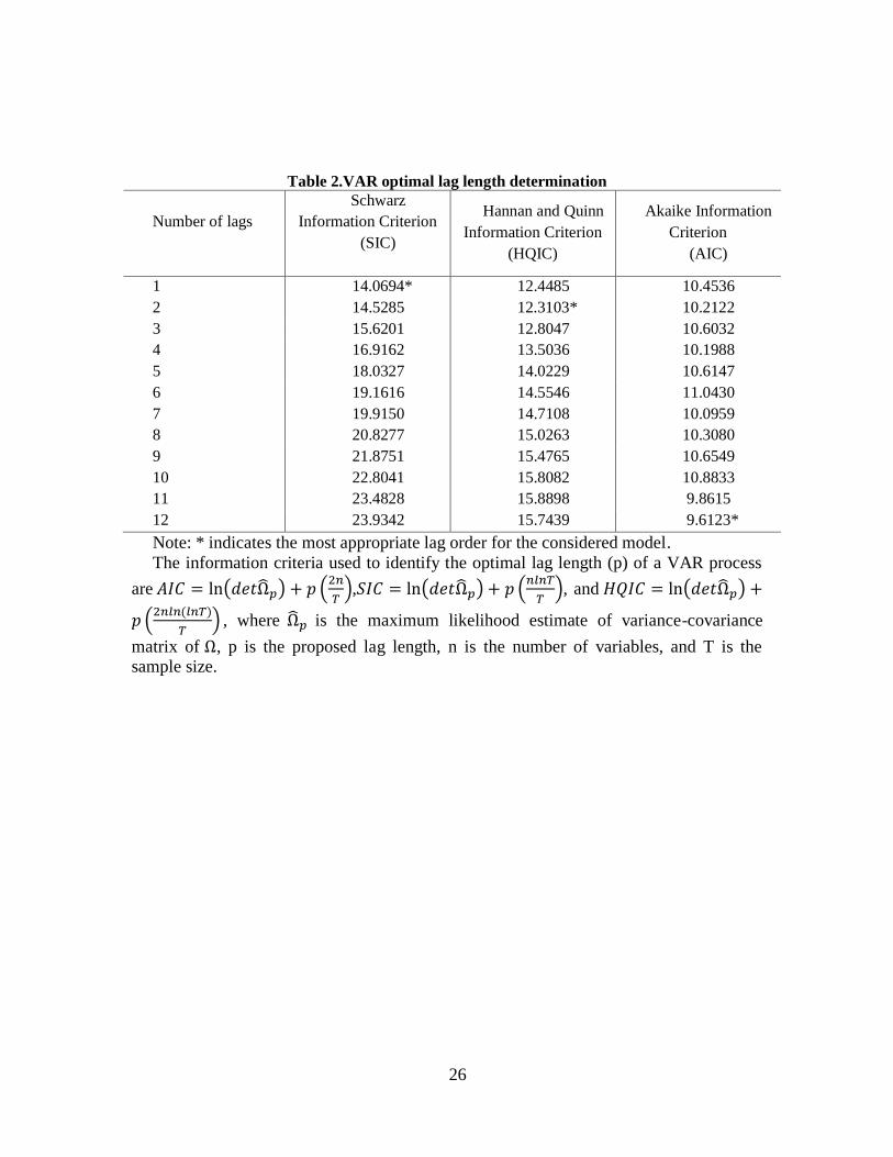
We use Schwarz loss, Akaike loss, Hannan and Quinn’s phi measures to determine the

optimal length of lags for the VAR model (Table 2). To find the optimal lag we tried

these tests for different set of regressions with seasonality, break and lags. We implement

the Bai-Parron break test and we choose ethanol production’s break at 2009:02. The

optimal lag length results shows smaller numbers with only seasonality and lags and not

break included. As one can see in this table, Schwarz loss, Hannan and Quinn’s phi

measures and Akaike loss are minimized at 1, 2 and 10 lags respectively. Smaller lag

length seems to be more reasonable for our study, so we need to choose between Schwarz

loss or Hannan and Quinn’s phi measures. We will use a two-lag VAR model suggested

14

by Hannan and Quinn’s phi measure since the Schwarz loss metric may have a tendency

to over-penalize additional regressors compared to the other metrics (Geweke and Meese

1981).

Estimation results of two-lag VAR

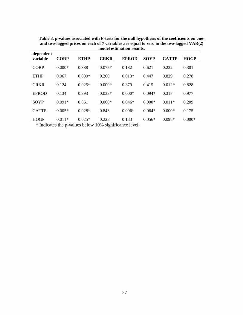
The p-values of F-test associated with the null hypothesis of both coefficients of one

and two-lagged prices jointly equal to zero at 10% level of statistical significance are

given in Table 3. As one can see in the table, all the variables have at least one other

significant coefficient in their equation, except for hog equation. Corn price coefficient is

significant in both ethanol price and ethanol production. Also corn price and ethanol

production are significant in crack ratio along with soybeans price coefficient. Soybeans,

Cattle and hog price coefficients are significant in five equations out of total of seven.

Ethanol price is only significant in ethanol production equation.

Identifying contemporaneous structure

We use LiNGAM algorithm to identify the causal structure of the variables in the

model. This algorithm is appropriate to use when at most one variable is Gaussian.

Therefore, the Normality test has been applied before using LiNGAM in this study. A

Jarque- Bera test has been applied to the data to determine whether they follow the

skewness and kurtosis matching a normal distribution or not. The test statistic is as

follows:

15

Where n is the number of observation, S is the sample skewness, and K is the sample

kurtosis. The results of the normality test are that we reject the null hypothesis of

normality for all the variables except for ethanol price.

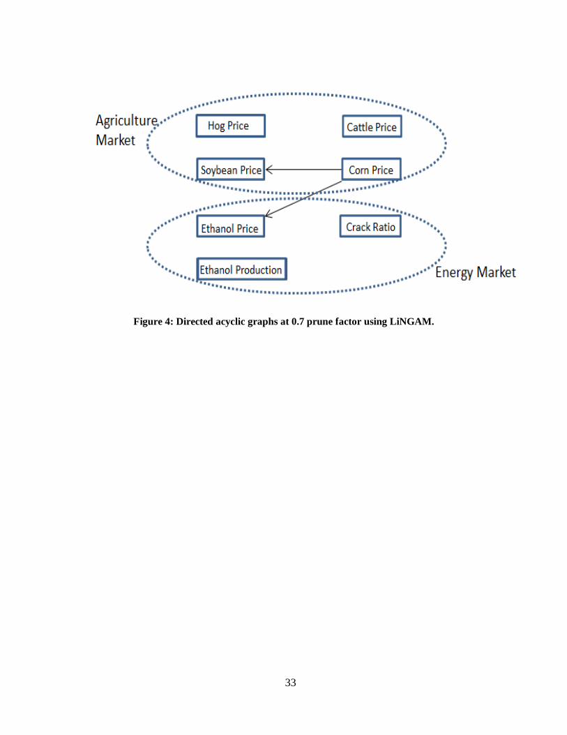
Using TETRAD (Scheines and Spirtes 1994) we implement LiNGAM algorithm with

prune factor 0.7 to figure out the contemporaneous structure among the seven variables.

Figure 4 represents causal structure among the variables of our model. As one can see in

this figure, energy and agriculture markets are connected through the edges between corn

price and ethanol price. The information flow is Corn price causes soybeans price and

also ethanol price.

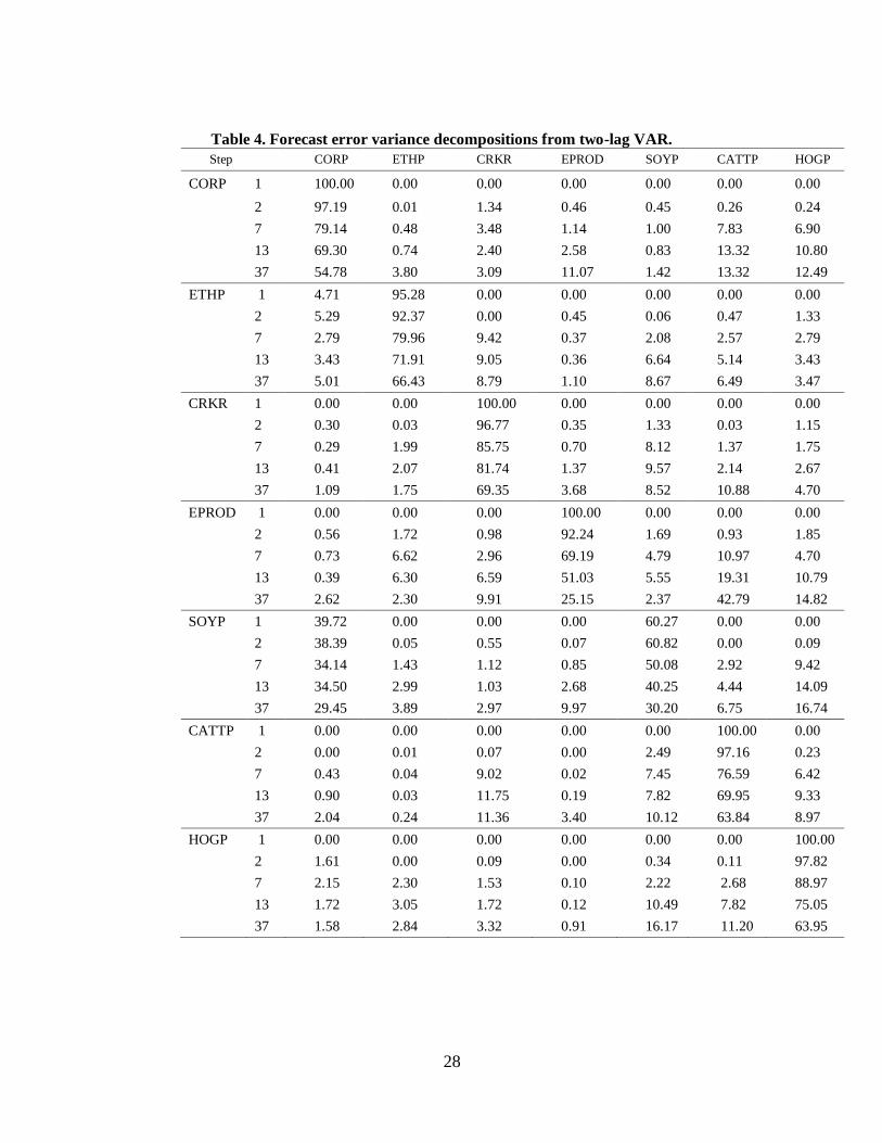
Forecast error variance decomposition

The results of forecast error variance decomposition are reported in table 4. The time

horizon of decompositions is zero (contemporaneous time), 1 month (short horizon), 6

months, 1 year and 3 years ahead (long term). The forecast error variance decomposition

suggests that that in contemporaneous time agriculture market prices are all exogenous,

except for soybeans which its variation is explained by innovations from corn (39.72%).

Variation of corn price in long horizon is explained mainly by ethanol production and

cattle price (11% and 13.3% respectively) and together with other variables they explain

50% of variation in corn price. In short run, the variations in cattle and hog prices are

accounted only by corn and soybeans price innovations and soybeans share is higher than

corn. But then in long term ethanol price and production and also crack ratio play role in

explaining cattle and hog prices. For instance, crack ratio and ethanol production explain

around 11% and 3.4% of cattle price respectively.

16

In energy market, crack ratio is showing exogeneity in contemporaneous time and the

variations in ethanol price are explained by itself mainly and also by corn price (4.7%).In

6 months horizon, Variations in ethanol price are explained by crack ratio for about 10%,

but this amount decreases in long run (3 years) to about 8.7%. we can see overall, share

of crack ratio in explaining ethanol price is higher than corn price in the longer term. And

the immediate effect of corn price on ethanol price is higher than crack ratio.

Moreover, although in short run the variables of the model only explain about 9% of

the variation in ethanol production but in long term (3years) this number increases to

about 75%. The main variables which describe ethanol production variation in long term

are crack ratio, cattle and hog prices.

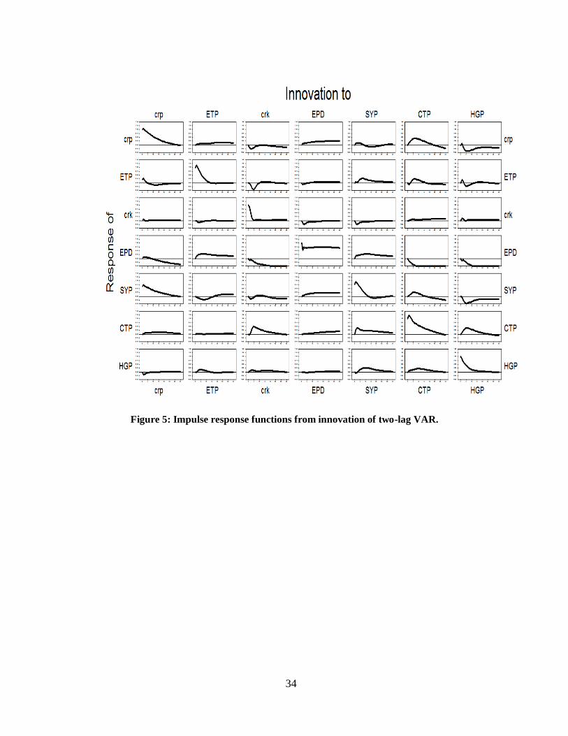
Innovation Accounting

We present impulse response functions to analyze the effects of a one-time only shock

of one of the series on the other series. One can see impulse response functions

represented in graph 5. Horizontal axes on the sub-graphs represent the horizon or

number of months after shock, which is 36 months in our study. Vertical axes show the

standardized response to the one time shock in each market. The variable’s names are

labeled at top of the columns.

As one can see in the graph 5, a shock in ethanol production transferred as a positive

and long lasting impulse to almost all of the agriculture market commodities’ prices

(corn, soybeans and cattle). Also in the energy market, a shock in ethanol production has

a negative influence on crack ratio, which dampens to zero in the long run. This means

increase in ethanol production decrease the gasoline refining margin and so gasoline price

17

relative to crude oil price. Also a shock in ethanol price will lead to a negative short term

impulse in crack ratio, which dampens to zero in longer term. Moreover the effects of a

shock to crack ratio on ethanol price is the same. The reason could be explained as when

the price of ethanol increases, demand of blended fuel will decrease and so do demand

and price of gasoline. Therefore ethanol price and gasoline price in short run are acting as

complementary goods. This also explains a negative response of corn price to one time

shock in crack ratio in short run. Increase in blended fuel price will lead to decrease in

demand of ethanol and also decrees in ethanol price and therefore corn price. Also as one

can see in the graph, the ethanol production will respond negatively to a shock in crack

ratio, which persists over the long term.

A positive shock of ethanol price also leads to a positive short impulse in hog

price. Part of this raise might be due to the long lasting increase of corn price, when

ethanol price shock happens. When ethanol price increases there might be more

incentives to allocate land to biofeedstocks instead of other crops which could be used as

food for livestock. This concept can also be seen as an increase in soybeans price after a

shock to ethanol production.

We note also a one-time shock in corn price will lead to short positive impulse to

ethanol price, since the ethanol production cost will increase. Also a shock to corn price

will lead to positive response of soybeans price. Since soybeans is an important grain for

animal feed, it could be a good substitute when price of corn increase. This excess

demand will affect the soybeans price to increase, and it gradually dampens to zero.

18

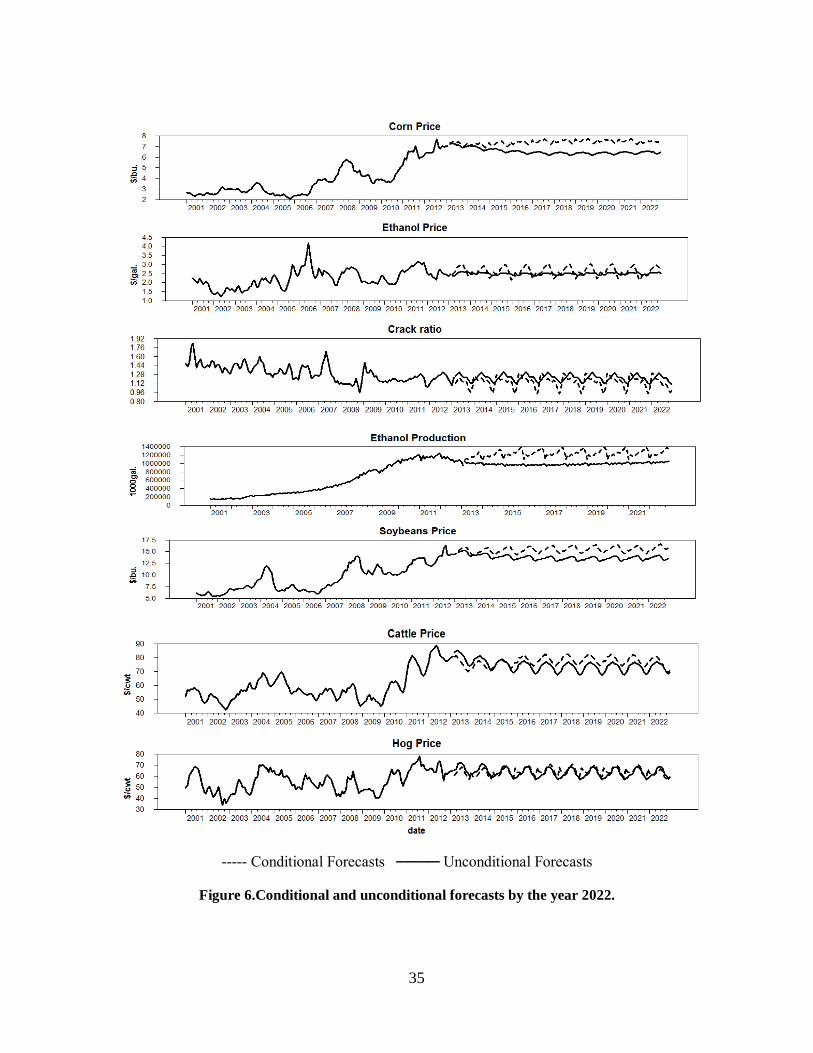
Forecasting and conditional forecasting

Forecasting exercises for prices has been performed by the year 2022. In our

forecasting we took in to account the Renewable Fuel Standards (RFS2) annual amount

of ethanol content in blended fuel with gasoline. RFS2 sets forth 13.8 and 14 billion

gallons of corn ethanol by 2013 and 2014 respectively. This amount will be fixed at 15

billion gallons from 2015 to 2022 to promote advanced biofuels, such as cellulosic

ethanol from switchgrass. The required amount of ethanol blended into fuel is declared

yearly, so we have calculated the required monthly amount by calculating the monthly

weights of ethanol production. Taking this mandatory amount of ethanol from RFS2 in

our model, we construct a conditional forecasting.

Comparing conditional and unconditional forecasts, one can see that all agricultural

commodities prices and ethanol price will be higher when we take into account for RFS

requirements in our model, except for hog prices and crack ratio. One can see the

forecasting results in the Error! Reference source not found.6. The solid line after Jan

2013 to the end of 2022 is the unconditional forecast and the dotted line is the forecast

conditional on RFS policies. Conditional forecasting gives us a corn price which is 15%

higher than unconditional forecast for the price average of 2022. This difference is 5%

for ethanol price and also 14% and 3.5% for soybeans and cattle prices. By contrast, the

conditional forecasts regarding RFS requirements leads to almost 6% lower gasoline

price than when there are no RFS requirements in the model.

In 2013, the blend wall limits ethanol consumption in E10 (motor gasoline contains

10%ethanol) to about 13.3 billion gallons (April 2013 short term Energy Outlook). For

19

this reason and also constant gasoline consumption of 138 billion gallons as in

predictions, ethanol falling short of required amount in the mandate (Coyle 2013;

Westcott and McPhail 2013). This extra amount of RFS was substituted by blending

advanced biofuels in excess of advanced RFS or by using accumulated credits (RINs)

(Irwin and Good 2013a). There are two ways to meet EPA requirement and expand the

blend wall: 1) increase in domestic gasoline consumption, 2) consumption of E15 or E85

instead of E10 (Irwin and Good 2013b). For this last one to happen we need a lower

ethanol price compare to gasoline price since a same amount of ethanol contains 25% less

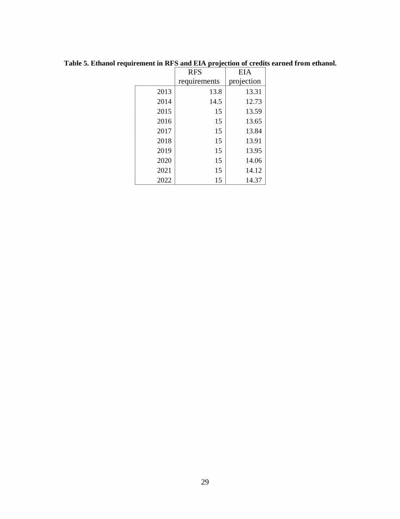
energy (Irwin and Good 2013a). At May 7th

2014, Energy Information Administration

had released a projection on (Irwin and Good 2013b)(Irwin and Good 2013b)(Irwin and

Good 2013b)(Irwin and Good 2013b)the amount of ethanol accredited to RFS (Annual

energy outlook 2014). One can compare the projection amount with RFS requirement in

table 5. We performed conditional forecasting on prices regarding EIA projection of

ethanol amount as well.

The average ethanol price for the year 2022 shows 4.8, 0.8, 2.8 percent decrease in corn,

ethanol and cattle price compare to the forecast conditional on RFS requirements. This

number is also showing 1% increase for crack ratio which together with ethanol price

decrease could make E85 more economically feasible.

20

Discussion

This study shows a significant linkage between agriculture and energy market through

corn. The results of directed acyclic graphs suggest that at contemporaneous time corn

causes soybeans price and ethanol price. Renewable fuel standards requirements and rise

in ethanol for demand affect the agriculture market.

Diversion of land to produce biofeedstocks and reduction in supply of other products

are some other issues regarding biofuels policies. Innovation accounting methods are

employed to summarize the integration between agriculture and energy markets.

Forecast error variance decomposition suggests that ethanol production explains about

10% of corn and soybeans prices in our model in longer term. These products count as a

feed for livestock as well, so their price rise has effects on livestock prices as well. Corn

price and soybeans price together count for about 12 and 18 percent of change in cattle

and hog prices.

Moreover crack ratio explains about 8.7% of ethanol price changes. Immediately after

a given positive shock to ethanol production the crack ratio will decrease. This could be

explained by the higher demand for ethanol. A rise in ethanol price will lead to higher

blended fuel price. The rise in blended fuel price then will lead to decrease in its demand.

This will also cause gasoline price to decrease. Impulse response results confirm that a

positive shock to ethanol price will decrease the crack ratio right after the shock, though

it dampens to zero, shortly after the pulse in ethanol price.

21

Finally we study conditional price forecasts taking RFS policies into account. Results

are showing higher prices for almost all the model’s commodities, and a lower crack

ratio, compare to no RFS restrictions forecasts by 2022.

Today Corn ethanol covers 10% of finished motor gasoline in US (E10). E85 (with

70-85% ethanol content) is consumed in limited volumes, and the infrastructure is not

prepared to increase this volume. One concern of today’s ethanol industry is that we have

reached a blending limit known as blending wall. That means reaching the RFS targets

for corn ethanol by 2022 will require raising the E10 blend standard for regular vehicles.

We have also performed a forecasting exercise regarding EIA projection of ethanol

accredited for RFS by 2022. The results indicate a smaller increase in ethanol price and a

larger decrease in gasoline price (both around 1%) compare to the forecasts conditioning

on RFS requirements.

22

References

Abbott, P.C., C. Hurt, and W.E. Tyner "What’s driving food prices in 2011?" (2011):

Alexander, C., and C. Hurt Biofuels and their impact on food pricesPurdue University

Cooperative Extension Service, 2007.

Awokuse, T.O., and D.A. Bessler "VECTOR AUTOREGRESSIONS, POLICY

ANALYSIS, AND DIRECTED ACYCLIC GRAPHS: AN APPLICATION TO THE US

ECONOMY." Journal of Applied Economics 6 (2003):

Bernanke, B. "Alternative explanations of the money-income correlation." Carnegie-

Rochester Conference Series on Public Policy no. 25, North-Holland, Amsterdam (1986):

Birur, D.K., T.W. Hertel, and W.E. Tyner "The biofuels boom: implications for world

food markets." The Food Economy Global Issues and Challenges.Wageningen:

Wageningen Academic Publishers (2009):61-75.

———"The biofuels boom: implications for world food markets." The Food Economy

Global Issues and Challenges.Wageningen: Wageningen Academic Publishers

(2009):61-75.

Bryant, H., and J. Outlaw "US Ethanol Production and Use Under Alternative Policy

Scenarios ." AFPC Research Report 06-1 (2006):

Carter, C., G. Rausser, and A. Smith "The effect of the US ethanol mandate on corn

prices." Unpublished manuscript (2012):

Cooley, T.F., and S.F. LeRoy "Atheoretical macroeconometrics: a critique." Journal

of Monetary Economics 16 (1985):283-308.

Coyle, W.T. "USDA Economic Research Service-Next-Generation Biofuels: Near-

Term Challenges and Implications for Agriculture." (2013):

Du, X., and D.J. Hayes "The impact of ethanol production on US and regional

gasoline markets." Energy Policy 37 (2009):3227-34.

Geweke, J., and R. Meese "Estimating regression models of finite but unknown

order." Journal of Econometrics 16 (1981):162.

Greene, W.H. Econometric analysisPearson Education India, 2003.

Hyvärinen, A., and E. Oja "Independent component analysis: algorithms and

applications." Neural Networks 13 (2000):411-30.

23

Irwin, S., and D. Good "The Ethanol Blend Wall, Biodiesel Production Capacity, and

the RFS...Something Has to Give." (2013a):

———"Expanding the Ethanol Blend Wall - a Role for E85?" (2013b):

Knittel, C., and A. Smith, "Ethanol production and gasoline prices: a spurious

correlation." (2012):

Pearl, J. "Causal diagrams for empirical research." Biometrika 82 (1995):669-88.

———Causality: models, reasoning and inferenceCambridge Univ Press, 2000.

Renewable Fuel Association "Renewable Fuel Standard."

http://www.ethanolrfa.org/pages/renewable-fuel-standard

Scheines, R., and P. Spirtes Tetrad II: Tools for Causal Modeling: User's Manual and

SoftwareLawrence Erlbaum Ass, 1994.

Shimizu, S., P.O. Hoyer, A. Hyvärinen, and A. Kerminen "A linear non-Gaussian

acyclic model for causal discovery." The Journal of Machine Learning Research 7

(2006):2003-30.

Sims, C.A., S.M. Goldfeld, and J.D. Sachs "Policy analysis with econometric models."

Brookings Papers on Economic Activity (1982):107-64.

Spirtes, P., C.N. Glymour, and R. Scheines Causation, prediction, and searchMIT

press, 2000.

Spirtes, P., C. Glymour, R. Scheines, and R. Tillman "Automated search for causal

relations: Theory and practice." (2010):

Tyner, W., F. Dooley, C. Hurt, and J. Quear "Ethanol pricing issues for 2008."

Industrial Fuels and Power 1 (2008):50-7.

Tyner, W.E. "The integration of energy and agricultural markets." Agricultural

Economics 41 (2010):193-201.

Tyner, W., and F. Taheripour "Biofuels, policy options, and their implications:

Analyses using partial and general equilibrium approaches." Journal of Agricultural &

Food Industrial Organization 6 (2008):

Westcott, P., and L. McPhail "USDA Economic Research Service-High RIN Prices

Suggest Market Factors Likely To Constrain Future US Ethanol Expansion." (2013):

24

———"USDA Economic Research Service-High RIN Prices Suggest Market Factors

Likely To Constrain Future US Ethanol Expansion." (2013):

Wisner, R. "Corn, ethanol and crude oil relationships implication for biofuels

industry." AgMRC Renewable Energy Newsletter (2009):

25

Table 1.Dickey–Fuller (DF) and Augmented Dickey–Fuller (ADF) for non-stationary of

variables.

The DF test is implemented through an ordinary least squares regression of the first

differences of prices on a constant and one lag of the levels of prices (Greene 2003). In

ADF test, k lags of dependent variable are included in the regression. The null hypothesis

for the test statistic of both tests is the data is non stationary in levels. The null hypothesis

is rejected when the observed t-statistics are less than this critical value. The 5% and

10% critical values are (-2.89, -2.58) (Fuller, 1976). ADF regression runs with 12 lags

and the chosen lag number (K) is the minimized Schwarz loss metric. Also the Q-

statistics is the Lung-Box statistics on the estimated residuals from the test regression.

The p-value with respect to each Q-statistics is given in the parenthesis.

Variables Dickey-Fuller Augmented Dickey-Fuller

Test Q Test K Q

Corn Price -0.29 62.23

(0.00)

-0.32 1 60.99

(0.00)

Ethanol Price -4.31 45.71

(0.12)

-2.84 2 31.18

(0.69)

Crack Ratio -5.15 70.42

(0.00)

-2.99 2 61.52

(0.00)

Ethanol Production 0.13 667.99

(0.00)

-0.08 1 249.14

(0.00)

Soybeans Price -1.43 70.78

(0.00)

-1.28 1 38.30

(0.36)

Cattle Price -2.46 302.88

(0.00)

-2.33 1 81.43

(0.00)

Hog Price -3.51 76.56

(0.00)

-3.30 1 71.05

(0.00)

26

Table 2.VAR optimal lag length determination

Number of lags

Schwarz

Information Criterion

(SIC)

Hannan and Quinn

Information Criterion

(HQIC)

Akaike Information

Criterion

(AIC)

1 14.0694* 12.4485 10.4536

2 14.5285 12.3103* 10.2122

3 15.6201 12.8047 10.6032

4 16.9162 13.5036 10.1988

5 18.0327 14.0229 10.6147

6 19.1616 14.5546 11.0430

7 19.9150 14.7108 10.0959

8 20.8277 15.0263 10.3080

9 21.8751 15.4765 10.6549

10 22.8041 15.8082 10.8833

11 23.4828 15.8898 9.8615

12 23.9342 15.7439 9.6123*

Note: * indicates the most appropriate lag order for the considered model.

The information criteria used to identify the optimal lag length (p) of a VAR process

are

,

, and

, where is the maximum likelihood estimate of variance-covariance

matrix of , p is the proposed lag length, n is the number of variables, and T is the sample size.

27

Table 3. p-values associated with F-tests for the null hypothesis of the coefficients on one-

and two-lagged prices on each of 7 variables are equal to zero in the two-lagged VAR(2)

model estimation results.

dependent

variable CORP ETHP CRKR EPROD SOYP CATTP HOGP

CORP 0.000* 0.388 0.075* 0.182 0.621 0.232 0.301

ETHP 0.967 0.000* 0.260 0.013* 0.447 0.829 0.278

CRKR 0.124 0.025* 0.000* 0.379 0.415 0.012* 0.828

EPROD 0.134 0.393 0.033* 0.000* 0.094* 0.317 0.977

SOYP 0.091* 0.861 0.060* 0.046* 0.000* 0.011* 0.209

CATTP 0.005* 0.028* 0.843 0.006* 0.064* 0.000* 0.175

HOGP 0.011* 0.025* 0.223 0.183 0.056* 0.098* 0.000*

* Indicates the p-values below 10% significance level.

28

Table 4. Forecast error variance decompositions from two-lag VAR.

Step CORP ETHP CRKR EPROD SOYP CATTP HOGP

CORP 1 100.00 0.00 0.00 0.00 0.00 0.00 0.00

2 97.19 0.01 1.34 0.46 0.45 0.26 0.24

7 79.14 0.48 3.48 1.14 1.00 7.83 6.90

13 69.30 0.74 2.40 2.58 0.83 13.32 10.80

37 54.78 3.80 3.09 11.07 1.42 13.32 12.49

ETHP 1 4.71 95.28 0.00 0.00 0.00 0.00 0.00

2 5.29 92.37 0.00 0.45 0.06 0.47 1.33

7 2.79 79.96 9.42 0.37 2.08 2.57 2.79

13 3.43 71.91 9.05 0.36 6.64 5.14 3.43

37 5.01 66.43 8.79 1.10 8.67 6.49 3.47

CRKR 1 0.00 0.00 100.00 0.00 0.00 0.00 0.00

2 0.30 0.03 96.77 0.35 1.33 0.03 1.15

7 0.29 1.99 85.75 0.70 8.12 1.37 1.75

13 0.41 2.07 81.74 1.37 9.57 2.14 2.67

37 1.09 1.75 69.35 3.68 8.52 10.88 4.70

EPROD 1 0.00 0.00 0.00 100.00 0.00 0.00 0.00

2 0.56 1.72 0.98 92.24 1.69 0.93 1.85

7 0.73 6.62 2.96 69.19 4.79 10.97 4.70

13 0.39 6.30 6.59 51.03 5.55 19.31 10.79

37 2.62 2.30 9.91 25.15 2.37 42.79 14.82

SOYP 1 39.72 0.00 0.00 0.00 60.27 0.00 0.00

2 38.39 0.05 0.55 0.07 60.82 0.00 0.09

7 34.14 1.43 1.12 0.85 50.08 2.92 9.42

13 34.50 2.99 1.03 2.68 40.25 4.44 14.09

37 29.45 3.89 2.97 9.97 30.20 6.75 16.74

CATTP 1 0.00 0.00 0.00 0.00 0.00 100.00 0.00

2 0.00 0.01 0.07 0.00 2.49 97.16 0.23

7 0.43 0.04 9.02 0.02 7.45 76.59 6.42

13 0.90 0.03 11.75 0.19 7.82 69.95 9.33

37 2.04 0.24 11.36 3.40 10.12 63.84 8.97

HOGP 1 0.00 0.00 0.00 0.00 0.00 0.00 100.00

2 1.61 0.00 0.09 0.00 0.34 0.11 97.82

7 2.15 2.30 1.53 0.10 2.22 2.68 88.97

13 1.72 3.05 1.72 0.12 10.49 7.82 75.05

37 1.58 2.84 3.32 0.91 16.17 11.20 63.95

29

Table 5. Ethanol requirement in RFS and EIA projection of credits earned from ethanol.

RFS

requirements

EIA

projection

2013 13.8 13.31

2014 14.5 12.73

2015 15 13.59

2016 15 13.65

2017 15 13.84

2018 15 13.91

2019 15 13.95

2020 15 14.06

2021 15 14.12

2022 15 14.37

30

Figure 1: Price index of agriculture and energy commodities.

0

1

2

3

4

5

6

Feb

-200

0

Sep

-200

0

Ap

r-20

01

No

v-20

01

Jun

-200

2

Jan

-200

3

Au

g-20

03

Mar

-200

4

Oct

-200

4

May

-200

5

Dec

-200

5

Jul-

2006

Feb

-200

7

Sep

-200

7

Ap

r-20

08

No

v-20

08

Jun

-200

9

Jan

-201

0

Au

g-20

10

Mar

-201

1

Oct

-201

1

May

-201

2

Dec

-201

2

ind

ex, j

an 2

000=

1

gasoline

Oil

ethanol

corn

31

Figure 2: Causal graph and reduced form- taken from Spirtes et al. 2010

32

Figure 3: Monthly time series plot (January2000- April 2013)

33

Figure 4: Directed acyclic graphs at 0.7 prune factor using LiNGAM.

34

Figure 5: Impulse response functions from innovation of two-lag VAR.

35

----- Conditional Forecasts ──── Unconditional Forecasts

Figure 6.Conditional and unconditional forecasts by the year 2022.