On the Dynamics of the Southern Senegal Upwelling Center

On the Dynamics of the Southern Senegal Upwelling Center: ObservedVariability from Synoptic to Superinertial Scales

XAVIER CAPET,a PHILIPPE ESTRADE,b ERIC MACHU,b,c SINY NDOYE,b,a JACQUES GRELET,d

ALBAN LAZAR,a LOUIS MARIÉ,c DENIS DAUSSE,a AND PATRICE BREHMERe,f

aLOCEAN Laboratory, CNRS-IRD-Sorbonne Universités, UPMC, MNHN, Paris, FrancebLaboratoire de Physique de l’Atmosphère et de l’Ocean Siméon Fongang, ESP/UCAD, Dakar, SenegalcLaboratoire d’Océanographie Physique et Spatiale, IRD-CNRS-IFREMER-UBO, Plouzané, France

d Institut de Recherche pour le Développement, US 191 IMAGO, Plouzané, Francee Institut Sénégalais de Recherche Agronomique, Centre de Recherche Océographique Dakar-Thiaroye,

Dakar, SenegalfLaboratoire des Sciences de l’Environnement Marin (UMR 195 LEMAR; IRD-CNRS-UBO-Ifremer),

Dakar, Senegal

(Manuscript received 2 December 2015, in final form 31 August 2016)

ABSTRACT

Upwelling off southern Senegal and Gambia takes place over a wide shelf with a large area where depths

are shallower than 20m. This results in typical upwelling patterns that are distinct (e.g., more persistent in

time and aligned alongshore) from those of other better known systems, including Oregon and Peru where

inner shelves are comparatively narrow. Synoptic to superinertial variability of this upwelling center is cap-

tured through a 4-week intensive field campaign, representing the most comprehensive measurements of this

region to date. The influence of mesoscale activity extends across the shelf break and far over the shelf where

it impacts the midshelf upwelling (e.g., strength of the upwelling front and circulation), possibly in concert

with wind fluctuations. Internal tides and solitary waves of large amplitude are ubiquitous over the shelf. The

observations suggest that these and possibly other sources of mixing play a major role in the overall system

dynamics through their impact upon the general shelf thermohaline structure, in particular in the vicinity of

the upwelling zone. Systematic alongshore variability in thermohaline properties highlights important limi-

tations of the 2D idealization framework that is frequently used in coastal upwelling studies.

1. Introduction

Coastal upwelling systems have received widespread

attention for several decades owing to their importance

for human society. Although the primary driving

mechanism is generic, important differences exist be-

tween systems and also between sectors of each given

system. Stratification, shelf/slope topographic shapes,

coastline irregularities, and subtleties in the wind spatial/

temporal structure have a major impact on upwelling

water pathways and overall dynamical, hydrological,

biogeochemical (Messié and Chavez 2015), and eco-

logical (Pitcher et al. 2010) characteristics of upwelling

regions. Over the past decade processes associated with

short time scales (daily and higher) have progressively

been incorporated into our knowledge base, adding

further complexity as we account for local specifics.

These advances have to a large extent taken place in

the California Current System (Woodson et al. 2007,

2009; Ryan et al. 2010; Kudela et al. 2008; Lucas et al.

2011a) and to a lesser extent in the Benguela system

(Lucas et al. 2014). Conversely, our understanding of

West African upwellings remains to a large extent su-

perficial (i.e., guided by satellite and sometimes surface

in situ measurements; Roy 1998; Demarcq and Faure

2000; Lathuilière et al. 2008), low frequency, and rela-

tively large scale. A notable exception is Schafstall et al.

(2010) with an estimation of diapycnal nutrient fluxes due

to internal wave dissipation over the Mauritanian shelf.

The large-scale dynamics and hydrology of the southern

end of the Canary system has, on the other hand, been

known for a long time (Barton 1998). Between the

Cape Verde frontal zone [which runs approximatelyCorresponding author e-mail: Xavier Capet, xclod@locean-ipsl.

upmc.fr

JANUARY 2017 CAPET ET AL . 155

DOI: 10.1175/JPO-D-15-0247.1

� 2017 American Meteorological SocietyUnauthenticated | Downloaded 04/09/22 02:04 PM UTC

mailto:[email protected]

mailto:[email protected]

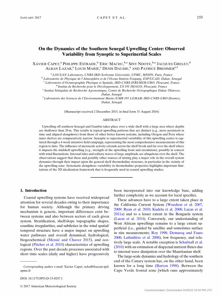
between Cape Blanc (;218N, Mauritania) and the

Cape Verde Archipelago (see Fig. 1)] and Cape

Roxo (128200N), the wind regime is responsible for

quasi-permanent Ekman pumping and winter/spring

coastal upwelling. The former extends hundreds of

kilometers offshore and drives a large-scale cyclonic cir-

culation whose manifestation includes the Mauritanian

Current (MC hereinafter; see Fig. 1). The MC differs

from poleward undercurrents typical of many upwelling

systems in that it is generally intensified at or close to the

surface (Peña-Izquierdo et al. 2012;Barton 1989), reflectingthe strength of the forcing. In the south, the MC connects

with the complex equatorial current system, and the con-

nection involves a quasi-stationary cyclonic feature: the

Guinea Dome [more details can be found in Barton (1998)

andAristegui et al. (2009)]. Figure 1 is suggestive of the role

of theMC inmaintaining a relatively warm environment in

the immediate vicinity of the shelf break over the latitude

band 128–178N, despite sustained coastal upwelling.

Seasonality of hydrology and circulation of the coastal

ocean off this part of West Africa are tightly controlled

by the displacements of the intertropical convergence

zone (Citeau et al. 1989). During the monsoon season

(July–October) weak westerly winds (interrupted by

the passage of occasional storms and easterly waves)

dominate and the region receives the overwhelming

fraction of its annual precipitation. From approxi-

mately November to May the ITCZ is located to the

south and upwelling-favorable trade winds dominate.

Their peak intensity is in February–April, our period of

interest, during which precipitation and river runoff is

insignificant.

Two coastal sectors can be distinguished in this region,

based on distinctions between their atmospheric forcings,

influence of the surrounding ocean, and shelf/slope

morphology. North of the Cape Verde Peninsula the

shelf is relatively narrow (up to the Banc d’Arguin at

;208N) and, because this is the northern limit of the

ITCZmigration, the upwelling season here is longest.

This study reports and analyzes observations carried

out in the southern sector offshore of southern Senegal

(between the Cape Verde Peninsula and;138400N; see

Fig. 1) during two consecutive field experiments

(amounting to 25 days at sea) carried out in February–

March 2013, that is, the core of the upwelling season.

The general strategy was to cover a relatively limited area

of;18 by 18 (Fig. 1) multiple times, taking measurements

of physical, biogeochemical, and ecological parameters.

We herein focus on the physics, but the role of this coastal

region as fishing ground and small pelagic fish nursery is an

important motivation for this work.

During the upwelling season, the southern sector

acts as an upwelling center referred to as southern

Senegal upwelling center (SSUC) below. The termi-

nology ‘‘upwelling center’’ refers to the existence of a

well-identified and persistent focal point where up-

welling is enhanced and from which a cold tongue

originates, as vividly revealed by SST images (Fig. 1). In

upwelling systems with intense mesoscale turbulence,

cold upwelling tongues take the form of filaments that

are predominantly directed toward the slope and open

ocean (Strub et al. 1991) and thus strongly contribute

to cross-shore exchanges. Mesoscale activity is not

particularly intense in the Canary system (Capet et al.

2008b; Marchesiello and Estrade 2009). In addition, the

SSUC is mostly characterized by a wide shelf. South of

148300N, the shelf break, roughly defined by the 100-m

isobath, is 50 km away from shore or more, while water

depth is less than 30m over 1/3 to 1/2 of the shelf area

(e.g., see Fig. 3). Thus, coastal upwelling in the SSUC is

partly sheltered from the mesoscale influence taking

place over the continental slope and open ocean. This

has several related implications: the general orientation

of the cold upwelling tongue is north to south and,

judging from SST images, it preserves its coherence over

long distances (up to 300–400km in some circumstances;

FIG. 1. Averaged Operational SST and Sea Ice Analysis (OSTIA)

composite SST over the northeastern tropical Atlantic for the

period 21 Feb–18 Mar 2013 corresponding to the UPSEN2–

ECOAO field experiments. The image was produced by averag-

ing daily fields downloaded online (from ftp://data.nodc.noaa.gov/

pub/data.nodc/ghrsst/L4/GLOB/UKMO/OSTIA). Superimposed

is a schematic representation of themain circulation features of the

region including the North Equatorial Countercurrent (NECC)

and the Cape Verde frontal zone (CVF, thick gray). Our study

area, the SSUC (black box), stands out as the southern tip of the

coastal upwelling system.White zonal lines indicate the location of

our three main hydrological transects.

156 JOURNAL OF PHYS ICAL OCEANOGRAPHY VOLUME 47

Unauthenticated | Downloaded 04/09/22 02:04 PM UTC

ftp://data.nodc.noaa.gov/pub/data.nodc/ghrsst/L4/GLOB/UKMO/OSTIA

ftp://data.nodc.noaa.gov/pub/data.nodc/ghrsst/L4/GLOB/UKMO/OSTIA

Ndoye et al. 2014);1 temporal stability of the tongue is

also noticeable over periods of many days to weeks; and

export from the shelf to the open ocean is retarded.

This being said, the degree of insulation between shelf

upwelling dynamics and offshore turbulent activity

needs to be qualified. South of 148300N, the upwelling

tongue is frequently found 50 km or more away from the

coast. Its offshore edge, generally referred to as the

upwelling front, is then within the range of influence of

large slope/shelfbreak eddies and meanders whose sur-

face expressions are frequently seen impinging on the

outer shelf (Ndoye et al. 2014). Such situations occur

preferentially between February and April and pre-

vailed during our observational period.2

The process underlying the offshore migration of the

upwelling tongue is present and well understood in 2D

across-shore/vertical (2DV) models. The key dynamical

feature of 2DV models subjected to upwelling-favorable

winds is the upwelling front.Under such idealizations, the

upwelling front possesses several defining characteristics

(Allen et al. 1995; Austin and Lentz 2002; Estrade et al.

2008): it is the physical barrier between offshore non-

upwelling and cold upwelling waters, that is, it is the place

of maximum surface density gradient (this can also be

true for other tracers); it is the place of maximum equa-

torward alongshore velocity; it coincides with the main

pycnocline outcrop (Austin and Barth 2002); and low/

vanishing stratification should be found on its inshore

flank, that is, the upwelling zone where cold interior

waters are incorporated into the surface layer.

Coalescence between the surface and bottom bound-

ary layers has traditionally been invoked as the main

explanation for the displacement of the upwelling front

away from the shoreline (Estrade et al. 2008; Austin and

Lentz 2002). In the alongshore momentum balance the

maintenance of well-mixed, inner-shelf waters implies a

compensation between wind and bottom friction with

little or no offshore Ekman transport needed. Therefore,

coastal divergence is expected to take place where water

is deep enough for the two boundary layers to separate,

typically 15 to 40m depending in part on wind intensity

(stronger winds lead to both thicker surface boundary

layers and thicker bottom boundary layers because they

tend to increase the strength of the upwelling jet (UJ) as

confirmed by the observations described below). In the

SSUC the migration of the upwelling tongue on seasonal

scales (very close to shore in the early season, farthest

offshore in March when upwelling winds are strongest,

and retreating back inshore in April–May) is consistent

with the cycle of upwelling wind intensity (Ndoye et al.

2014). On the other hand, analysis of SSUC SST also

shows cold upwelling tongue behavior (in terms of zonal

position and displacements) that is suggestive of other

processes being at play. Farther north, over a wide con-

tinental shelf resembling the SSUC, Barton et al. (1977)

observe an upwelling front that migrates offshore during

two consecutive upwelling events without any evident

relation to changes in wind intensity. Similar behavior

will be described below for the SSUC. Overall, the con-

nection between cross-shore migration of the upwelling

zone and wind intensity is unclear, at least on synoptic

time scales.

The purpose of this study is to better understand the

dynamics underlying upwelling front evolutions and,

more generally, shed light on the dynamics of the SSUC.

As we will see, other aspects of the 2DV conceptual

model that have traditionally been used to investigate the

SSUC dynamics need serious reconsideration in the light

of the Upwelling du Sénégal 2 (UPSEN2)–Écosystèmes

de l’Afrique de l’Ouest (ECOAO) observations. Identi-

fication of the upwelling front during these experiments is

frequently ambiguous, and, when possible, the upwelling

front rarely satisfies all of the characteristics laid out

above. Also, limited sampling of the inshore edge of the

upwelling tongue suggests that warmer coastal waters

were overwhelmingly stratified during the experiments;

hence, the 2DV view of the offshore migration of the

upwelling tongue does not seem to be relevant.

On the other hand, our observations provide multiple

pieces of evidence pointing to the importance of

complex-scale interactions in the SSUC. Shelfbreak/

open-ocean mesoscale disturbances and superinertial

dynamics (e.g., internal gravity waves) exert a funda-

mental influence on the SSUC dynamics, thermohaline

structure, and, in particular, on the position and shape of

the upwelling tongue.

The manuscript is organized as follows: Section 2

presents the data and methods. Section 3 describes the

synoptic evolution of the SSUC state and circulation

1Note, however, that incorporation of subsurface water in the

tongue tens to hundreds of kilometers from its northern origin near

Dakar cannot be ruled out. In other words the concept of a wake,

within which upwelled water in a confined northern area would

simply be advected southward, may not be applicable. In that re-

spect, the cold tongue may be distinct from upwelling filaments

present in other upwelling sectors in which the key dynamical

process is subduction of recently upwelled water as it flows offshore

past the shelf break.2 The seaward displacement of the cold tongue is accompanied

by the establishment of a nearshore, warm-water strip south of

;148200N that has historically attracted much attention because it

is, intuitively, favorable to the retention of eggs and larvae of

marine species (Demarcq and Faure 2000). The shallow and poorly

charted area where this warm strip is found was considered unsafe

for the R/V Antéa. Therefore, just a small number of observations

were made at the edge of this strip, which does not allow us to

properly analyze its dynamics.



during the field experiments. Emphasis is placed on the

midshelf area where moored instruments allow us to

better characterize the dynamics. The flow regime and

submesoscale activity are also briefly examined. In section

4, a set of observations is presented from ship echosounders

and moored instruments that suggests the dynamical im-

portance of the SSUC internal wave field. The final section

summarizes and elaborates on our findings and their

consequences.

2. Data and methods

a. Moored instruments

A string of instruments (hereinafter referred to as

M28) was deployed in about 28-m water depth at 148N,

178060W on 23 February (0800 UTC) and recovered on

12 March (1500 UTC). It consisted of 8 temperature T

sensors and 10 temperature, salinity S, and pressure sen-

sors with a 1-min sampling interval. Measurements made

by the 18T sensors are used to obtain a temperature time–

depth gridded field (described in sections 3 and 4). This is

achieved through objective analysis (Bretherton et al.

1976), using 1m and 2min for the vertical and time res-

olution of the grid and 1m and 4min for the decorrelation

depth and time scale. The decorrelation time scale is

chosen so that internal wave signals with periods of

;10min or more are preserved.

Three upward-looking ADCP moorings were also

deployed 0.5nmwest and east (RDI 300kHz respectively

referred to as RDIW and RDIE) and south [Aquadopp

400kHz (AQDS)] of the thermistor line. Mean water

depth at the moorings ranged from approximately 29

(RDIW) to 26.5m (RDIE). One additional ADCP

Aquadopp 600kHz (AQDI) was moored a few miles to

the east in 23-m depth. Deployment of the ADCPs took

place on 22 February between 1020 and 1210 UTC. Re-

covery took place on 12 (RDIW) or 15 March. RDI

(Aquadopp) ADCPs sampled every 2min (5min) with

vertical resolution of 1m. Accounting for the depth at

which the instrument’s head was located (’0.5m above

ground) and a 1-m blanking distance, the lowest valid

measurement is centered at 2m above the bottom. Be-

cause of sidelobe reflection from the air–sea interface, the

shallowest useable bin is centered at 5-m depth. The

barotropic component of measured currents was detided

using the software T_Tide (Pawlowicz et al. 2002). M2 is

by far the dominant constituent (not shown).

b. Hydrographic measurements

Zonal (approximately across shore) CTD transects

were repeated at 148, 148300, and 138400N during the

surveys and additional yoyo CTD stations were also

performed. Data were acquired using a SBE9111, re-

dundantly measuring pressure, temperature, and con-

ductivity at 24Hz and fluorescence and oxygen at 2Hz.

Data postprocessing was performed using the SeaBird

SBE processing software and follows standard practices

as described in many studies (see, e.g., Morison et al.

1994). Only the downcast profiles are used for analysis;

during the upcast sensors are in the wake of the package

and CTD frame (Alford and Pinkel 2000). Raw pressure

is filtered using a 15-point triangle window. This is

enough to eliminate all pressure reversals despite the

relatively low drop speed we chose to increase vertical

resolution (0.5m s21). We attribute this to CTD opera-

tion through a moon pool located toward the center of

R/V Antéa, which limits heave effects. Sea states were

also favorable with limited swell in the area. A 5-point

median filter is applied to temperature and salinity. A

correction for the conductivity cell thermal mass

(Morison et al. 1994) is also applied, requiring the

knowledge of two parameters a (initial amplitude) and t

(time scale) that characterize conductivity measurement

error when instantaneously applying a 18C step in tem-

perature. SBE default values were checked and slightly

modified using a series of profiles exhibiting abrupt T

jumps at the interface of a well-mixed, 20–30-m-thick

bottom layer (not shown). The salinity profile closest

to a step was obtained for a 5 0.025 and t 5 7 s, and

these values are used for all CTD profiles. For most

purposes including the construction of hydrological

transects, depth averaging is performed over 1-m bins.

Bin size is reduced to 0.15m to construct yoyo CTD

profiles used to estimate dissipation and mixing in-

tensity, through the computation of Thorpe scales

(section 4). This roughly corresponds to seven scans at

the drop speed of 0.5m s21.

Alongtrack surface temperature and salinity are

available from the SBE21 ship thermosalinometer (TSG

data hereinafter).

c. Ancillary measurements

R/VAntéa is equippedwith a four-frequency scientificechosounder SIMRADEK60 (38, 70, 120, and 200 kHz).

The ping rate is 1Hz, which yields a 3.5-m native reso-

lution for the echograms when the ship steams at 8 knots

(kt; 1 kt 5 0.51ms21).

The weather station onboard R/VAntéa (Batos 1.1D)

provides wind speed and direction measured at ap-

proximately 20-m height. To minimize the effect of

airflow distortion by the ship superstructure, measure-

ments corresponding to aft wind conditions are sys-

tematically discarded. Hourly wind at the Yoff weather

station at Dakar Airport, Senegal (148440N, 178300W,

27m above ground; hereinafter DWS) are obtained



online (from http://www.ogimet.com/metars.phtml.en).

ASCAT scatterometers onboard Meteorological Oper-

ational (MetOp)-A and MetOp-B provide 2D wind

measurements between zero and three times a day,

around 1030 and/or 2230 UTC. We use the 12.5-km L2

products from NASA and present these observations

after spatial averaging over different subdomains of

the SSUC.

We use L2 Moderate Resolution Imaging Spectror-

adiometer (MODIS) onboard the Terra and Aqua sat-

ellites distributed by NASA (http://oceancolor.gsfc.

nasa.gov). The metric ground resolution varies de-

pending on view angle but remains close to the nominal

1-km value. Cloud masking produces numerous false

positives in upwelling regions, and we instead rely on

visual examination over the SSUC to keep or discard

images.

3. Subinertial SSUC dynamics

Several types of observations, presented below, give

complementary perspectives on the physical situation

during the campaigns and, particularly, on the sequence

of synoptic events.

a. Synoptic variability

DWS is generally quite representative of synoptic

wind conditions over the SSUC, especially in situations

where northwesterlies dominate (Ndoye et al. 2014), as

during UPSEN2–ECOAO. Analysis of DWS wind re-

cords (Fig. 2a) suggest three coherent subperiods:

a moderate relaxation periodRL1 from the beginning of

the cruise (22 February) to 27 February when the wind

over the previous inertial period is back to above 5ms21;

28 February to 12 March (UP1) during which the wind

intensity remains essentially between 5 and 7ms21; and

from 12 March to 17–18 March during which another

relaxation period RL2 takes place that, beside a more

rapid initiation and a longer duration (;5 days vs

3–4 days), resembles the earlier one RL1. The short

upwelling event that took place around 20–21 February

just before UPSEN2 is referred to as UP0.

This description of DWS winds is broadly consistent

with ship weather station observations made within

50km of M28 reported in Fig. 2d. For example, the

weakest (strongest) ship winds are found on 25 February

and 15 March (28 February and 8 March). This being

said, limited coverage at M28 and significant intradaily

variability tend to overshadow the synoptic signal and

curtail a detailed comparison. In particular, daily wind

cycles differ at M28 and DWS. During most of the ex-

periment, upwelling wind intensity at M28 peaks in the

evening or early at night and is at minimum around

midday (Fig. 2e). Also note that upwelling events seem

to manifest themselves through increased maximum

wind intensities at M28, while morning winds remain

generally weak. The daily wind cycle has a much lower

amplitude at DWS and maximum wind intensity occurs

around 1400 UTC (see Ndoye et al. 2014).

In Fig. 2b, we show the zonal minimum temperature

over the shelf averaged over the latitudinal range

148–148300N, computed for all cloud-free MODIS SST

images (a subset of these images is presented in Fig. 3).

The upwelling event finished around the beginning

ofUPSEN2UP0; the short relaxation periodRL1, central

upwelling event UP1, and final relaxation RL2 are

clearly identifiable as SST fluctuations of ;28–38C. Thetermination date of RL1 cannot be determined precisely

in SST because no MODIS SST is available on 25 and

26 February, but declining temperatures on 27–28 Feb-

ruary approximately coincide with the increase in up-

welling wind intensity. As for the SST warming during

the late part of the observation period, its initiation

around 8 March precedes the marked wind drop on 12–

13 March by around 4 days. We will come back to this

discrepancy when presenting midshelf variability. In

SST RL2 is most marked on 17 March, that is, upon the

return of more favorable upwelling wind conditions.

Overall, the storylines based on DWS winds or

synoptic evolution of the system SST are in good

agreement, considering the sampling limitations and

complexity of the ocean response to wind changes.

b. SSUC mesoscale variability

With over 50 nearly cloud-free images over the du-

ration of the experiment, MODIS provides invaluable

information on the state and synoptic variability of the

SSUC at scales of a few kilometers and larger.

Most images exhibit the patterns typical of the SSUC

during the upwelling season, namely, the presence of a

tongue of cold water whose source is situated just south

of Dakar (where the coldest waters are found) and ex-

tends southward over the shelf, with some warmer wa-

ters being found offshore but also inshore of the tongue

south of 148300N. Southward attenuation of the cold

signal strongly varies with time.

During the entire experiment, the frontal zone be-

tween the cold upwelling water and warmer offshore

water is distorted and forms filaments and meanders of

typical size ;20–100km, some of which acquire quasi-

circular shapes (Fig. 3). As demonstrated for other up-

welling systems these mesoscale structures must be the

manifestation of baroclinic–barotropic instability

(Marchesiello et al. 2003). The tendency of filaments to

orient themselves along a northwest–southeast axis

(Figs. 3e–h) reflects the intense lateral shear (partly



http://www.ogimet.com/metars.phtml.en

http://oceancolor.gsfc.nasa.gov

http://oceancolor.gsfc.nasa.gov

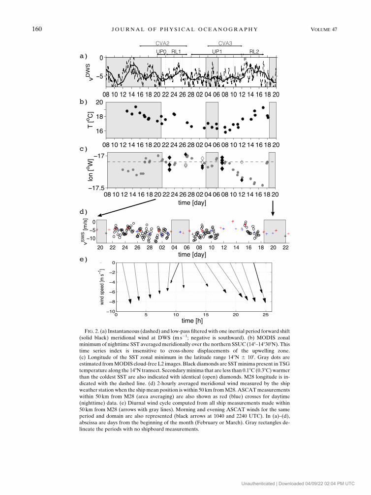
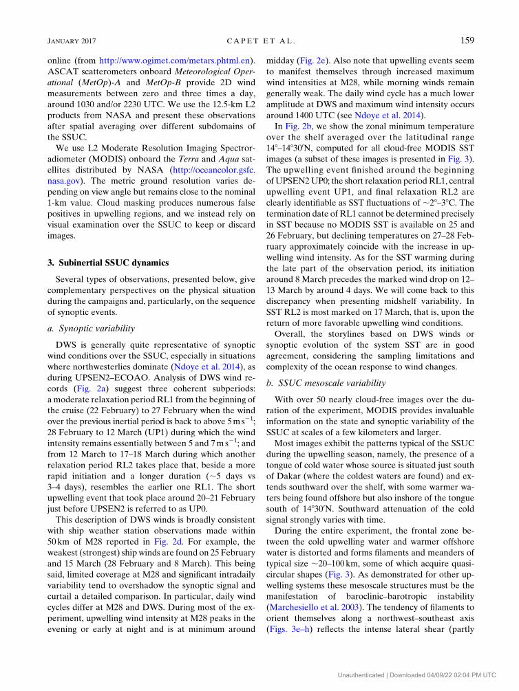
FIG. 2. (a) Instantaneous (dashed) and low-pass filteredwith one inertial period forward shift

(solid black) meridional wind at DWS (m s21; negative is southward). (b) MODIS zonal

minimumof nighttime SST averagedmeridionally over the northern SSUC (148–148300N). This

time series index is insensitive to cross-shore displacements of the upwelling zone.

(c) Longitude of the SST zonal minimum in the latitude range 148N 6 100. Gray dots are

estimated fromMODIS cloud-free L2 images. Black diamonds are SSTminima present in TSG

temperature along the 148N transect. Secondaryminima that are less than 0.18C (0.38C)warmer

than the coldest SST are also indicated with identical (open) diamonds. M28 longitude is in-

dicated with the dashed line. (d) 2-hourly averaged meridional wind measured by the ship

weather station when the shipmean position is within 50 km fromM28. ASCATmeasurements

within 50 km from M28 (area averaging) are also shown as red (blue) crosses for daytime

(nighttime) data. (e) Diurnal wind cycle computed from all ship measurements made within

50 km from M28 (arrows with gray lines). Morning and evening ASCAT winds for the same

period and domain are also represented (black arrows at 1040 and 2240 UTC). In (a)–(d),

abscissa are days from the beginning of the month (February or March). Gray rectangles de-

lineate the periods with no shipboard measurements.



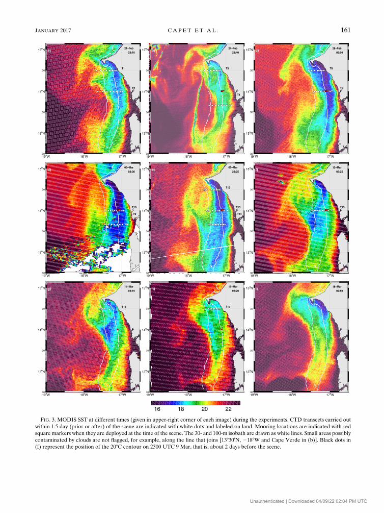
FIG. 3. MODIS SST at different times (given in upper-right corner of each image) during the experiments. CTD transects carried out

within 1.5 day (prior or after) of the scene are indicated with white dots and labeled on land. Mooring locations are indicated with red

square markers when they are deployed at the time of the scene. The 30- and 100-m isobath are drawn as white lines. Small areas possibly

contaminated by clouds are not flagged, for example, along the line that joins [138300N, 2188W and Cape Verde in (b)]. Black dots in

(f) represent the position of the 208C contour on 2300 UTC 9 Mar, that is, about 2 days before the scene.



resolved by our across-shore sections; see below) be-

tween the poleward Mauritanian Current and the in-

shore equatorward upwelling flow.

In their analysis of the MODIS SST database, Ndoye

et al. (2014) identify a recurrent mesoscale situation

when a 30–100-km anticyclone [referred to as the Cape

Verde anticyclone (CVA) structure] hugs the Cape

Verde headland. In February–March 2013 three differ-

ent CVAs consecutively occupy the northern SSUC

following a sequence of events involving 1) northward

propagation anddeformation/amplificationof aMauritanian

Current meander initially situated farther south; 2)

phase locking or reduced propagation of the meander,

which remains in the immediate vicinity of the Cape

Verde headland for several days while taking a more cir-

cular shape; and 3) weakening/shrinking of the structure

in a fashion that suggests mixing between warm waters in

the CVA core and colder waters.

At the beginning of UPSEN2 (21–23 February) the

remains of a small CVA (CVA-2) more easily identified

at earlier times (18 February, not shown) are still visible

50 km to the south-southwest of Cape Verde (Fig. 3a).

On 27 February (Fig. 4), the SST signal of CVA-2 has

mostly faded. The SST scene for 28 February (Fig. 3c)

captures the transient situation when ;188C water oc-

cupies the vicinity of Cape Verde and warmer water is

located;30km farther offshore. It also reveals the final

stage of the evacuation of CVA-2, which has been stir-

red beyond recognition in the deformation region near

148450N, 178450W, and the northward progression of

the frontal edge oriented northwest–southeast that

separates a warm MC meander from upwelling water

between 138400N and 148500N (cf. Figs. 3b and 3c). This

frontal zone had remained quasi stationary from 21 to

24–25 February. By 3 March, it has shifted considerably

farther north (Fig. 3d). It is then located partly north of

and in close contact with Cape Verde. The northern and

southern parts of the front evolve somewhat indepen-

dently thereafter. North of Cape Verde, the front

progresses northward and forms a barrier to cold upw-

elled water (Fig. 3e), even right at the coast where SSTs

are systematically warmer than 208C during UP1. South

of Cape Verde the front combines with a ;208C water

filament located at 178450–188W to form the quasi-

circular edge of a mesoscale structure (CVA-3) be-

tween 5 and 10–12 March (Figs. 3e,f).

The SST signature of CVA-3 is progressively eroded,

particularly at its eastern side as seen on 12 March

(Fig. 3f). On 14 March (Fig. 3g), the remains of CVA-3

are barely visible as a bulge of ;208C water near

148300N, 178450W. Later on, during RL2 (Figs. 3h,i), SST

images reveal a major reorganization of the flow struc-

ture in the vicinity of the Cape Verde Peninsula. The

upwelling signature on SST is confined to the northern

SSUC (note that the maintenance of some upwelling is

consistent with DWS and ship wind records; see Fig. 2).

The orientation of the wake of waters upwelled at the

Cape Verde Peninsula suggests that the surface flow is

directed offshore on 18 March in the region between

the coast and a subsequent warmmeander still situated

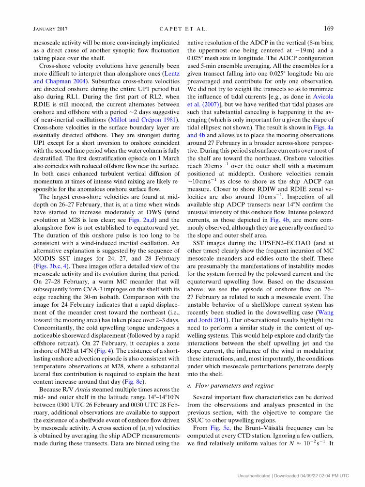
FIG. 4. (top) MODIS SST and (middle) ship ADCP velocities

(across shore u, alongshore y) around 27 Feb during an episode of

intense onshore flow. (bottom)The number of individual transects

contributing to every binned velocity data is also indicated.



approximately 50km offshore to the southwest (Fig. 3i).

VIIRS ocean color images available for 17 and 18 March

further support the onset of an offshore surface flow

in the northern SSUC toward the end of RL2 (not

shown).

The mesoscale features described above are typically

located over the continental slope, but they also fre-

quently extend onto the shelf as described below using

in situ observations. Their evolution is tied to that of the

SSUC cold tongue over the shelf, for example, through

upwelling filaments. Pending modeling sensitivity ana-

lyses, our conceptual view of the SSUC dynamics is that

offshore and shelf dynamics are coupled through the

instabilities of the shelf/shelfbreak/slope current system.

Synoptic variabilities of the MC transport and of the

wind-induced shelf circulation are a priori important

sources of modulation for these instabilities.

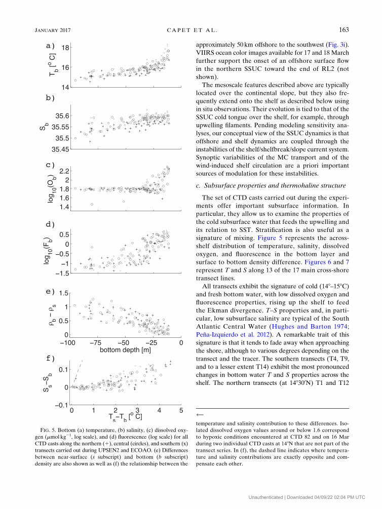
c. Subsurface properties and thermohaline structure

The set of CTD casts carried out during the experi-

ments offer important subsurface information. In

particular, they allow us to examine the properties of

the cold subsurface water that feeds the upwelling and

its relation to SST. Stratification is also useful as a

signature of mixing. Figure 5 represents the across-

shelf distribution of temperature, salinity, dissolved

oxygen, and fluorescence in the bottom layer and

surface to bottom density difference. Figures 6 and 7

represent T and S along 13 of the 17 main cross-shore

transect lines.

All transects exhibit the signature of cold (148–158C)and fresh bottom water, with low dissolved oxygen and

fluorescence properties, rising up the shelf to feed

the Ekman divergence. T–S properties and, in parti-

cular, low subsurface salinity are typical of the South

Atlantic Central Water (Hughes and Barton 1974;

Peña-Izquierdo et al. 2012). A remarkable trait of this

signature is that it tends to fade away when approaching

the shore, although to various degrees depending on the

transect and the tracer. The southern transects (T4, T9,

and to a lesser extent T14) exhibit the most pronounced

changes in bottom water T and S properties across the

shelf. The northern transects (at 148300N) T1 and T12

FIG. 5. Bottom (a) temperature, (b) salinity, (c) dissolved oxy-

gen (mmol kg21, log scale), and (d) fluorescence (log scale) for all

CTD casts along the northern (1), central (circles), and southern (x)

transects carried out during UPSEN2 and ECOAO. (e) Differences

between near-surface (s subscript) and bottom (b subscript)

density are also shown as well as (f) the relationship between the

temperature and salinity contribution to these differences. Iso-

lated dissolved oxygen values around or below 1.6 correspond

to hypoxic conditions encountered at CTD 82 and on 16 Mar

during two individual CTD casts at 148N that are not part of the

transect series. In (f), the dashed line indicates where tempera-

ture and salinity contributions are exactly opposite and com-

pensate each other.



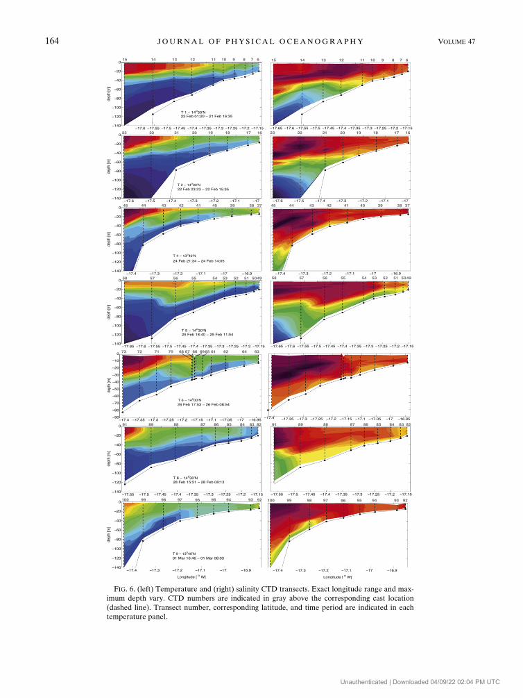
FIG. 6. (left) Temperature and (right) salinity CTD transects. Exact longitude range and max-

imum depth vary. CTD numbers are indicated in gray above the corresponding cast location

(dashed line). Transect number, corresponding latitude, and time period are indicated in each

temperature panel.



are those where bottomwater T and S properties are best

preserved. Although this does not apply to T8 it confirms

the visual impression from the SST images that the shelf is

preferentially fed with slope waters in the northern

SSUC. Many studies document the effect of capes and

changes in shelf width on upwelling pathways and

strength, which adds support to the visual impression

(Gan and Allen 2002; Pringle 2002; Pringle and Dever

2009; Gan et al. 2009; Crépon et al. 1984). Ongoing

modeling work specific to the area is also supportive of

this (Ndoye 2016).

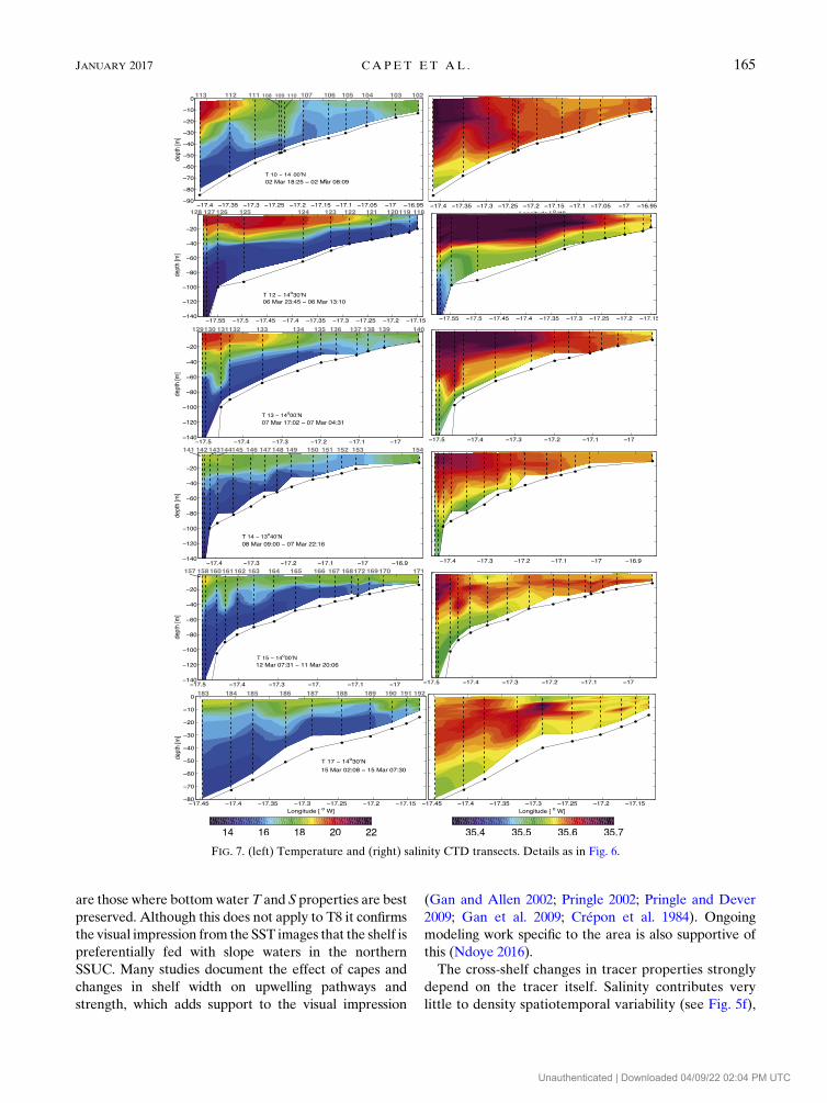
The cross-shelf changes in tracer properties strongly

depend on the tracer itself. Salinity contributes very

little to density spatiotemporal variability (see Fig. 5f),

FIG. 7. (left) Temperature and (right) salinity CTD transects. Details as in Fig. 6.



but its fluctuations over the shelf are nonetheless mea-

surable and provide useful indications on mixing. Sa-

linity and temperature experience marked relative

changes between the shelf break and the 15-m isobath.

The changes are most pronounced over the outer shelf

for salinity with a tendency to saturation at about

35.6 psu for depths shallower than 40–50m (Fig. 5b).

The cross-shore structure is reversed for temperature

with the most significant changes occurring at depths

shallower than 30m. However, the warming trend from

deep to shallow parts of the shelf is ubiquitous. For

dissolved oxygen, changes are very limited at depths

greater than ;30m and generally consist in a slight re-

duction from offshore to nearshore. For shallower

depths, a large variability is found, particularly at the

central and southern transects. Changes in fluorescence

resemble those for oxygen, although they are less con-

centrated to the shallowest depths; for example, the

outer shelf variability is much more pronounced.

Modification of bottom water biogeochemical prop-

erties when getting closer to shore goes in pair with a

reduction in surface to bottom stratification (Figs. 5e,f),

which occasionally vanishes inshore of the 30-m isobath.

This points to the importance of vertical mixing as a

process controlling the distribution of water column

properties. Other processes shape the mean tracer dis-

tribution and in particular sources and sinks. We pre-

sume that biological activity is able to maintain sharp

vertical contrasts in oxygen and fluorescence between

the upper 20–40m and the layer below and prevent

mixing from significantly affecting the vertical distribu-

tion of these two tracers. For example, ventilation

through mixing is unable to prevent hypoxia from de-

veloping toward the end of ECOAO during the re-

laxation period (see the three low dissolved oxygen

outliers in Fig. 5c). This and other synoptic anoxic/

hypoxic events are under investigation, similar to what is

being done in other upwelling regions (Adams et al.

2013). Conversely, the absence of interior source/sink

for temperature and salinity allows vertical mixing to

have a significant impact on these fields.

Other aspects of the SSUC thermohaline structure

suggest the importance of mixing. As mentioned in the

introduction, the key dynamical feature of idealized

upwelling models is their well-identifiable upwelling

front, located where the main pycnocline outcrops and

separates upwelling and nonupwelling waters. The

complexity of the SSUC upwelling structure leads to

equivocal situations regarding the definition/localization

of the upwelling front and zone. In particular, the sur-

face temperature and salinity across-shore gradients

are frequently weak and diffuse, for example, 28Cover 25 km for T1, from CTD6 to CTD12. A notable

exception is found during T6 (148N) where a 1.48Cchange was observed over a horizontal distance of

250m. Other exceptions are described in detail below as

part of a submesoscale activity analysis.

More importantly, choosing a density/temperature

value characteristic of the offshore pycnocline and fol-

lowing it toward the coast to its outcropping position

does not reliably help define the location of the up-

welling front, in contrast to, for example, what happens

over the Oregon shelf (Austin and Barth 2002). The

main reason for this is that considerable changes in

stratification and thermohaline structure occur across

the shelf, not just in the bottom layer as described above

but also at middepth. Manifestations of intense mixing

of thermocline waters include the presence of bulges

of water in temperature classes that are almost un-

represented offshore (CTD43 in T4, CTD55–56 in T5,

CTD70 in T6, CTD108–111 in T10, and CTD163

in T15).

In other words, except at the northern transects T1,

T8, and T12 [which exhibit clear upwelling frontal

structures as found, e.g., offshore of Oregon in Huyer

et al. (2005)] and at the southern T14 [which resembles

the idealized 2DV upwelling in Estrade et al. (2008) and

Austin and Lentz (2002)], the exact location where up-

welling is taking place is difficult to identify precisely.

For example, T6 has a strong surface temperature gra-

dient and an almost well-mixed water column at

178100W near CTD 66–69, but a significant amount of

cold bottom water resides inshore of that location. A

more dramatic example is obtained for T15 at the end of

upwelling event UP1. On 12 March the upwelling front

location at 148N, determined as the place of zonal min-

imum SST (from MODIS SST in Fig. 2c or TSG data,

not shown), sits around 178250W in 75-m water depth

near CTD 163. On the other hand, a secondary SST

minimum (see Fig. 2c) is found much closer to shore

near M28, and the cold bottom water resides over most

of the shelf, including at mooring M28 (see Fig. 8).

We attribute this complexity of the shelf thermoha-line structure properties to intense vertical mixing.Although bottom friction may be also implicated, wepresent evidence that internal gravity waves breakingshould play an important role as a source of mixing insection 4.

d. Midshelf dynamics

The description above can be complemented by and

contrasted with the continuous current and temperature

measurements available at 148N about the 28-m isobath,

although records cover a restricted period from23February

to 12 or 15March. Inwhat follows, heat content is defined asÐ zszbrCp(T2Tm) dz, where Cp is the heat capacity of water



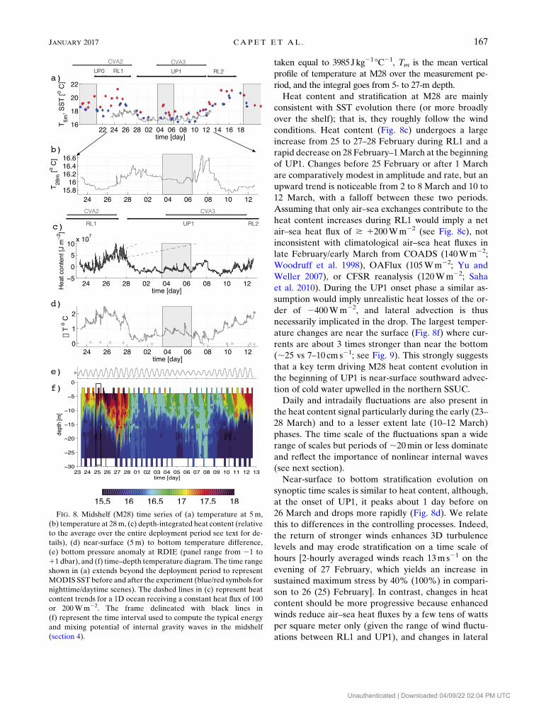
taken equal to 3985Jkg21 8C21, Tm is the mean vertical

profile of temperature at M28 over the measurement pe-

riod, and the integral goes from 5- to 27-m depth.

Heat content and stratification at M28 are mainly

consistent with SST evolution there (or more broadly

over the shelf); that is, they roughly follow the wind

conditions. Heat content (Fig. 8c) undergoes a large

increase from 25 to 27–28 February during RL1 and a

rapid decrease on 28 February–1March at the beginning

of UP1. Changes before 25 February or after 1 March

are comparatively modest in amplitude and rate, but an

upward trend is noticeable from 2 to 8 March and 10 to

12 March, with a falloff between these two periods.

Assuming that only air–sea exchanges contribute to the

heat content increases during RL1 would imply a net

air–sea heat flux of * 1200Wm22 (see Fig. 8c), not

inconsistent with climatological air–sea heat fluxes in

late February/early March from COADS (140Wm22;

Woodruff et al. 1998), OAFlux (105Wm22; Yu and

Weller 2007), or CFSR reanalysis (120Wm22; Saha

et al. 2010). During the UP1 onset phase a similar as-

sumption would imply unrealistic heat losses of the or-

der of 2400Wm22, and lateral advection is thus

necessarily implicated in the drop. The largest temper-

ature changes are near the surface (Fig. 8f) where cur-

rents are about 3 times stronger than near the bottom

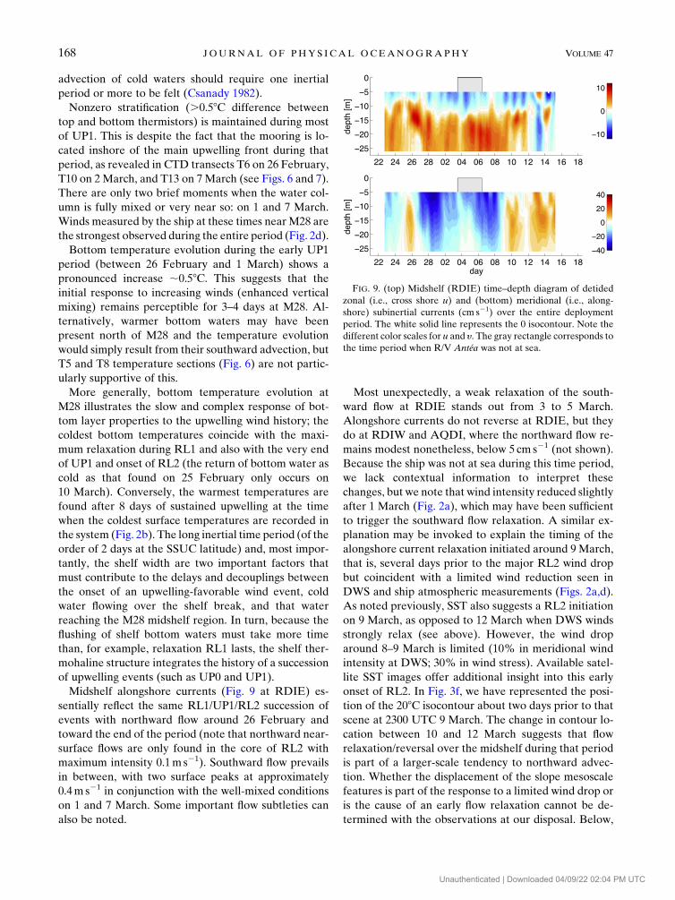
(;25 vs 7–10 cm s21; see Fig. 9). This strongly suggests

that a key term driving M28 heat content evolution in

the beginning of UP1 is near-surface southward advec-

tion of cold water upwelled in the northern SSUC.

Daily and intradaily fluctuations are also present in

the heat content signal particularly during the early (23–

28 March) and to a lesser extent late (10–12 March)

phases. The time scale of the fluctuations span a wide

range of scales but periods of ;20min or less dominate

and reflect the importance of nonlinear internal waves

(see next section).

Near-surface to bottom stratification evolution on

synoptic time scales is similar to heat content, although,

at the onset of UP1, it peaks about 1 day before on

26 March and drops more rapidly (Fig. 8d). We relate

this to differences in the controlling processes. Indeed,

the return of stronger winds enhances 3D turbulence

levels and may erode stratification on a time scale of

hours [2-hourly averaged winds reach 13m s21 on the

evening of 27 February, which yields an increase in

sustained maximum stress by 40% (100%) in compari-

son to 26 (25) February]. In contrast, changes in heat

content should be more progressive because enhanced

winds reduce air–sea heat fluxes by a few tens of watts

per square meter only (given the range of wind fluctu-

ations between RL1 and UP1), and changes in lateral

FIG. 8. Midshelf (M28) time series of (a) temperature at 5m,

(b) temperature at 28m, (c) depth-integrated heat content (relative

to the average over the entire deployment period see text for de-

tails), (d) near-surface (5m) to bottom temperature difference,

(e) bottom pressure anomaly at RDIE (panel range from 21 to

11 dbar), and (f) time–depth temperature diagram. The time range

shown in (a) extends beyond the deployment period to represent

MODIS SST before and after the experiment (blue/red symbols for

nighttime/daytime scenes). The dashed lines in (c) represent heat

content trends for a 1D ocean receiving a constant heat flux of 100

or 200Wm22. The frame delineated with black lines in

(f) represent the time interval used to compute the typical energy

and mixing potential of internal gravity waves in the midshelf

(section 4).



advection of cold waters should require one inertial

period or more to be felt (Csanady 1982).

Nonzero stratification (.0.58C difference between

top and bottom thermistors) is maintained during most

of UP1. This is despite the fact that the mooring is lo-

cated inshore of the main upwelling front during that

period, as revealed in CTD transects T6 on 26 February,

T10 on 2 March, and T13 on 7 March (see Figs. 6 and 7).

There are only two brief moments when the water col-

umn is fully mixed or very near so: on 1 and 7 March.

Winds measured by the ship at these times near M28 are

the strongest observed during the entire period (Fig. 2d).

Bottom temperature evolution during the early UP1

period (between 26 February and 1 March) shows a

pronounced increase ;0.58C. This suggests that the

initial response to increasing winds (enhanced vertical

mixing) remains perceptible for 3–4 days at M28. Al-

ternatively, warmer bottom waters may have been

present north of M28 and the temperature evolution

would simply result from their southward advection, but

T5 and T8 temperature sections (Fig. 6) are not partic-

ularly supportive of this.

More generally, bottom temperature evolution at

M28 illustrates the slow and complex response of bot-

tom layer properties to the upwelling wind history; the

coldest bottom temperatures coincide with the maxi-

mum relaxation during RL1 and also with the very end

of UP1 and onset of RL2 (the return of bottom water as

cold as that found on 25 February only occurs on

10 March). Conversely, the warmest temperatures are

found after 8 days of sustained upwelling at the time

when the coldest surface temperatures are recorded in

the system (Fig. 2b). The long inertial time period (of the

order of 2 days at the SSUC latitude) and, most impor-

tantly, the shelf width are two important factors that

must contribute to the delays and decouplings between

the onset of an upwelling-favorable wind event, cold

water flowing over the shelf break, and that water

reaching the M28 midshelf region. In turn, because the

flushing of shelf bottom waters must take more time

than, for example, relaxation RL1 lasts, the shelf ther-

mohaline structure integrates the history of a succession

of upwelling events (such as UP0 and UP1).

Midshelf alongshore currents (Fig. 9 at RDIE) es-

sentially reflect the same RL1/UP1/RL2 succession of

events with northward flow around 26 February and

toward the end of the period (note that northward near-

surface flows are only found in the core of RL2 with

maximum intensity 0.1m s21). Southward flow prevails

in between, with two surface peaks at approximately

0.4m s21 in conjunction with the well-mixed conditions

on 1 and 7 March. Some important flow subtleties can

also be noted.

Most unexpectedly, a weak relaxation of the south-

ward flow at RDIE stands out from 3 to 5 March.

Alongshore currents do not reverse at RDIE, but they

do at RDIW and AQDI, where the northward flow re-

mains modest nonetheless, below 5 cm s21 (not shown).

Because the ship was not at sea during this time period,

we lack contextual information to interpret these

changes, but we note that wind intensity reduced slightly

after 1 March (Fig. 2a), which may have been sufficient

to trigger the southward flow relaxation. A similar ex-

planation may be invoked to explain the timing of the

alongshore current relaxation initiated around 9 March,

that is, several days prior to the major RL2 wind drop

but coincident with a limited wind reduction seen in

DWS and ship atmospheric measurements (Figs. 2a,d).

As noted previously, SST also suggests a RL2 initiation

on 9 March, as opposed to 12 March when DWS winds

strongly relax (see above). However, the wind drop

around 8–9 March is limited (10% in meridional wind

intensity at DWS; 30% in wind stress). Available satel-

lite SST images offer additional insight into this early

onset of RL2. In Fig. 3f, we have represented the posi-

tion of the 208C isocontour about two days prior to that

scene at 2300 UTC 9 March. The change in contour lo-

cation between 10 and 12 March suggests that flow

relaxation/reversal over the midshelf during that period

is part of a larger-scale tendency to northward advec-

tion. Whether the displacement of the slope mesoscale

features is part of the response to a limited wind drop or

is the cause of an early flow relaxation cannot be de-

termined with the observations at our disposal. Below,

FIG. 9. (top) Midshelf (RDIE) time–depth diagram of detided

zonal (i.e., cross shore u) and (bottom) meridional (i.e., along-

shore) subinertial currents (cm s21) over the entire deployment

period. The white solid line represents the 0 isocontour. Note the

different color scales for u and y. The gray rectangle corresponds to

the time period when R/V Antéa was not at sea.



mesoscale activity will be more convincingly implicated

as a direct cause of another synoptic flow fluctuation

taking place over the shelf.

Cross-shore velocity evolutions have generally been

more difficult to interpret than alongshore ones (Lentz

and Chapman 2004). Subsurface cross-shore velocities

are directed onshore during the entire UP1 period but

also during RL1. During the first part of RL2, when

RDIE is still moored, the current alternates between

onshore and offshore with a period ;2 days suggestive

of near-inertial oscillations (Millot and Crépon 1981).

Cross-shore velocities in the surface boundary layer are

essentially directed offshore. They are strongest during

UP1 except for a short inversion to onshore coincident

with the second time periodwhen thewater column is fully

destratified. The first destratification episode on 1 March

also coincides with reduced offshore flow near the surface.

In both cases enhanced turbulent vertical diffusion of

momentum at times of intense wind mixing are likely re-

sponsible for the anomalous onshore surface flow.

The largest cross-shore velocities are found at mid-

depth on 26–27 February, that is, at a time when winds

have started to increase moderately at DWS (wind

evolution at M28 is less clear; see Figs. 2a,d) and the

alongshore flow is not established to equatorward yet.

The duration of this onshore pulse is too long to be

consistent with a wind-induced inertial oscillation. An

alternative explanation is suggested by the sequence of

MODIS SST images for 24, 27, and 28 February

(Figs. 3b,c, 4). These images offer a detailed view of the

mesoscale activity and its evolution during that period.

On 27–28 February, a warm MC meander that will

subsequently form CVA-3 impinges on the shelf with its

edge reaching the 30-m isobath. Comparison with the

image for 24 February indicates that a rapid displace-

ment of the meander crest toward the northeast (i.e.,

toward the mooring area) has taken place over 2–3 days.

Concomitantly, the cold upwelling tongue undergoes a

noticeable shoreward displacement (followed by a rapid

offshore retreat). On 27 February, it occupies a zone

inshore ofM28 at 148N (Fig. 4). The existence of a short-

lasting onshore advection episode is also consistent with

temperature observations at M28, where a substantial

lateral flux contribution is required to explain the heat

content increase around that day (Fig. 8c).

Because R/VAntéa steamedmultiple times across the

mid- and outer shelf in the latitude range 148–148100Nbetween 0300 UTC 26 February and 0030 UTC 28 Feb-

ruary, additional observations are available to support

the existence of a shelfwide event of onshore flow driven

by mesoscale activity. A cross section of (u, y) velocities

is obtained by averaging the ship ADCP measurements

made during these transects. Data are binned using the

native resolution of the ADCP in the vertical (8-m bins;

the uppermost one being centered at 219m) and a

0.0258 mesh size in longitude. The ADCP configuration

used 5-min ensemble averaging. All the ensembles for a

given transect falling into one 0.0258 longitude bin are

preaveraged and contribute for only one observation.

We did not try to weight the transects so as to minimize

the influence of tidal currents [e.g., as done in Avicola

et al. (2007)], but we have verified that tidal phases are

such that substantial canceling is happening in the av-

eraging (which is only important for u given the shape of

tidal ellipses; not shown). The result is shown in Figs. 4a

and 4b and allows us to place the mooring observations

around 27 February in a broader across-shore perspec-

tive. During this period subsurface currents over most of

the shelf are toward the northeast. Onshore velocities

reach 20 cm s21 over the outer shelf with a maximum

positioned at middepth. Onshore velocities remain

;10 cm s21 as close to shore as the ship ADCP can

measure. Closer to shore RDIW and RDIE zonal ve-

locities are also around 10 cm s21. Inspection of all

available ship ADCP transects near 148N confirm the

unusual intensity of this onshore flow. Intense poleward

currents, as those depicted in Fig. 4b, are more com-

monly observed, although they are generally confined to

the slope and outer shelf area.

SST images during the UPSEN2–ECOAO (and at

other times) clearly show the frequent incursion of MC

mesoscale meanders and eddies onto the shelf. These

are presumably the manifestations of instability modes

for the system formed by the poleward current and the

equatorward upwelling flow. Based on the discussion

above, we see the episode of onshore flow on 26–

27 February as related to such a mesoscale event. The

unstable behavior of a shelf/slope current system has

recently been studied in the downwelling case (Wang

and Jordi 2011). Our observational results highlight the

need to perform a similar study in the context of up-

welling systems. This would help explore and clarify the

interactions between the shelf upwelling jet and the

slope current, the influence of the wind in modulating

these interactions, and, most importantly, the conditions

under which mesoscale perturbations penetrate deeply

into the shelf.

e. Flow parameters and regime

Several important flow characteristics can be derived

from the observations and analyses presented in the

previous section, with the objective to compare the

SSUC to other upwelling regions.

From Fig. 5e, the Brunt–Väisälä frequency can be

computed at every CTD station. Ignoring a few outliers,

we find relatively uniform values for N ’ 1022 s21. It



yields deformation radius values ranging from’8 km at

midshelf to 27 km at the shelf break, that is, on the

higher end of what is typically found in upwellings. This

is mainly because the Coriolis parameter is small ( f 53.63 1025 s21 at 148300N). The topographic slope along

all three transects is also quite uniform a ’ 2 3 1023.

The resulting slopeBurger numberB5 (aN)/f is around

0.5. In a steady 2Dupwelling, theway the return onshore

flow balancing offshore Ekman transport is achieved

depends on B (Lentz and Chapman 2004). A value of B

smaller (greater) than 1 implies that the wind stress is

balanced by bottom friction (nonlinear across-shelf flux

of alongshore momentum), so the return flow is con-

centrated in the bottom boundary layer (distributed in

the water column below the surface boundary layer);

B 5 0.5 suggests the importance of frictional forces in

the alongshore momentum balance but is comparable to

values found offshore of Oregon and northern Cal-

ifornia, where both the topographic slope and Coriolis

frequency are larger (Lentz and Chapman 2004). The

prominence of the cold bottom layer rising up the shelf

in most T–S transects (Figs. 6, 7) is qualitatively con-

sistent with this.

Geostrophy is an important force balance that the

nontidal part of the flow should approximately satisfy.

Tidally filtered RDIE currents at M28 described above

exhibit substantial fluctuations on time scales of 1 day or

less, particularly in the alongshore direction (Fig. 9).

This suggests that deviations from geostrophy are im-

portant, and the subinertial flow is characterized by

Rossby numbers that are not negligibly small compared

to 1. Because wind fluctuations do not conclusively ex-

plain several rapid flow changes, we tend to see this as a

manifestation of the submesoscale dynamics in the

upwelling zone.

Submesoscale turbulence consists of fronts, small

eddies, and filaments with typical horizontal scales& Rd

(where Rd is the first deformation radius) and a strong

tendency to near-surface intensification. Key processes

for submesoscale generation are (Capet et al. 2008d)

(i) straining/frontogenesis by mesoscale structures,

which intensifies preexisting buoyancy contrasts and

leads to fronts whose vertical scale is typically that of the

mesoscale, and (ii) straining/frontogenesis by finescale

parallel flow instabilities, which distorts mesoscale

buoyancy gradients and produces submesoscale flows

whose vertical scale can bemuch smaller than that of the

mesoscale. An archetypal example of point ii is mixed

layer baroclinic instability, which generates sub-

mesoscale flow fluctuations approximately confined into

the mixed layer (Boccaletti et al. 2007; Capet et al.

2008d). In their most extreme manifestations, contrasts

across submesoscale fronts can reach several degrees

over lateral scales of 50–100m. Such contrasts are the

consequence of intense straining in situations where

diffusion is weak.

Upwelling dynamics are well known to induce intense

submesoscale frontal activity, but some precision is in

order to connect with our SSUC study. Submesoscale

fronts are ubiquitous in the offshore coastal transition

zone where cold upwelled and warm offshore waters are

being stirred (Flament et al. 1985; Capet et al. 2008c;

Pallàs-Sanz et al. 2010). Our study is concerned with

shelf dynamics where the interaction between cold up-

welling and warmer offshore waters is strongly con-

strained by topography, friction, and inertia–gravity

wave (IGW) breaking. A numerical investigation of the

northern Argentinian shelf dynamics indicates that the

submesoscale is strongly damped in water depths shal-

lower than ;50m (Capet et al. 2008a) and the same

should apply to the SSUC; hence, we expect limited

submesoscale turbulence over the inner- and midshelf.

On the other hand, the upwelling front is frequently

located over the outer shelf where it can be subjected to

straining by CVAs so it is a priori conducive to the

formation of submesoscale features.

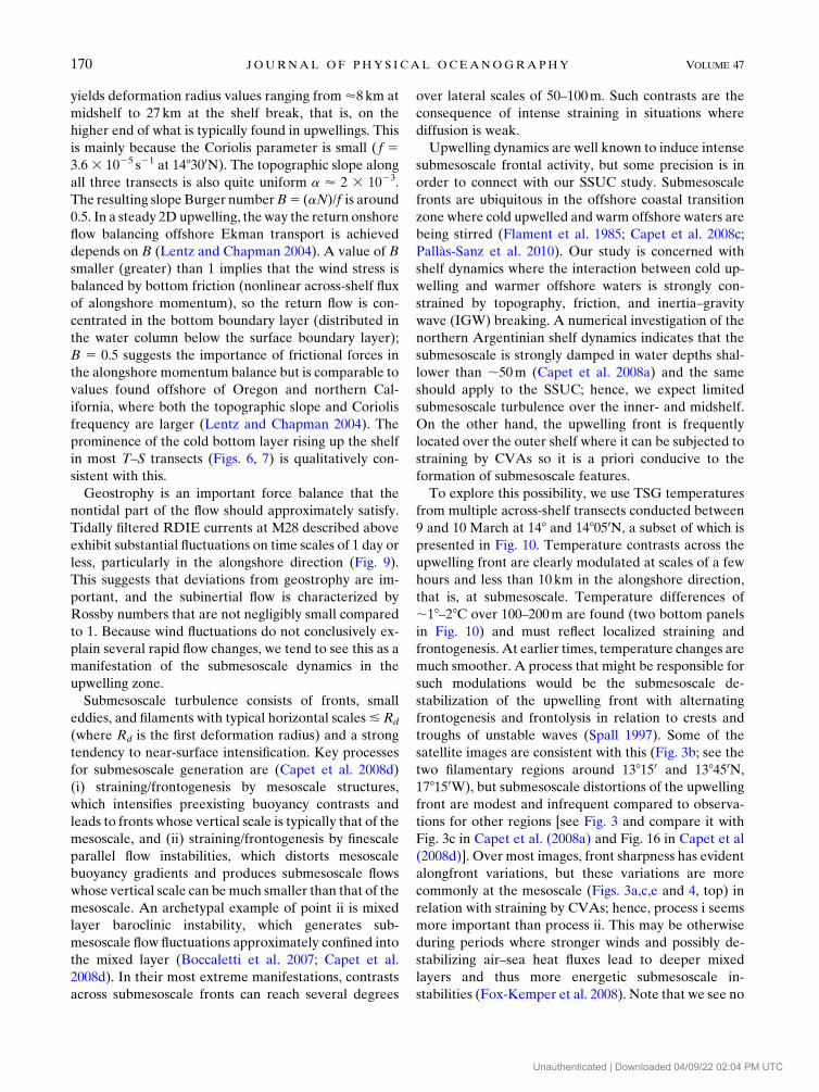
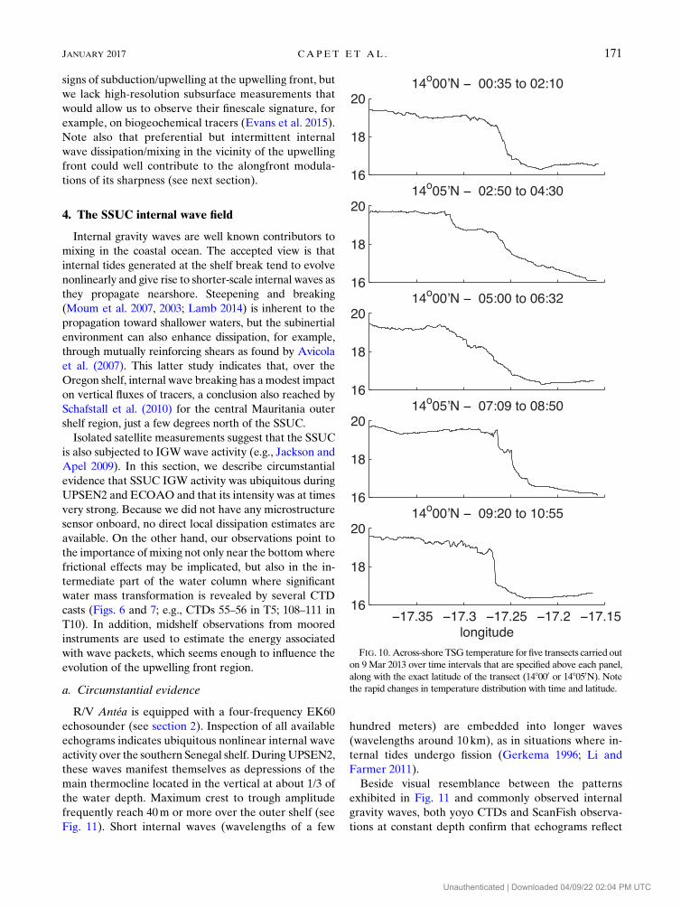
To explore this possibility, we use TSG temperatures

from multiple across-shelf transects conducted between

9 and 10 March at 148 and 148050N, a subset of which is

presented in Fig. 10. Temperature contrasts across the

upwelling front are clearly modulated at scales of a few

hours and less than 10km in the alongshore direction,

that is, at submesoscale. Temperature differences of

;18–28C over 100–200m are found (two bottom panels

in Fig. 10) and must reflect localized straining and

frontogenesis. At earlier times, temperature changes are

much smoother. A process that might be responsible for

such modulations would be the submesoscale de-

stabilization of the upwelling front with alternating

frontogenesis and frontolysis in relation to crests and

troughs of unstable waves (Spall 1997). Some of the

satellite images are consistent with this (Fig. 3b; see the

two filamentary regions around 138150 and 138450N,

178150W), but submesoscale distortions of the upwelling

front are modest and infrequent compared to observa-

tions for other regions [see Fig. 3 and compare it with

Fig. 3c in Capet et al. (2008a) and Fig. 16 in Capet et al

(2008d)]. Over most images, front sharpness has evident

alongfront variations, but these variations are more

commonly at the mesoscale (Figs. 3a,c,e and 4, top) in

relation with straining by CVAs; hence, process i seems

more important than process ii. This may be otherwise

during periods where stronger winds and possibly de-

stabilizing air–sea heat fluxes lead to deeper mixed

layers and thus more energetic submesoscale in-

stabilities (Fox-Kemper et al. 2008). Note that we see no



signs of subduction/upwelling at the upwelling front, but

we lack high-resolution subsurface measurements that

would allow us to observe their finescale signature, for

example, on biogeochemical tracers (Evans et al. 2015).

Note also that preferential but intermittent internal

wave dissipation/mixing in the vicinity of the upwelling

front could well contribute to the alongfront modula-

tions of its sharpness (see next section).

4. The SSUC internal wave field

Internal gravity waves are well known contributors to

mixing in the coastal ocean. The accepted view is that

internal tides generated at the shelf break tend to evolve

nonlinearly and give rise to shorter-scale internal waves as

they propagate nearshore. Steepening and breaking

(Moum et al. 2007, 2003; Lamb 2014) is inherent to the

propagation toward shallower waters, but the subinertial

environment can also enhance dissipation, for example,

through mutually reinforcing shears as found by Avicola

et al. (2007). This latter study indicates that, over the

Oregon shelf, internal wave breaking has amodest impact

on vertical fluxes of tracers, a conclusion also reached by

Schafstall et al. (2010) for the central Mauritania outer

shelf region, just a few degrees north of the SSUC.

Isolated satellite measurements suggest that the SSUC

is also subjected to IGW wave activity (e.g., Jackson and

Apel 2009). In this section, we describe circumstantial

evidence that SSUC IGW activity was ubiquitous during

UPSEN2 and ECOAO and that its intensity was at times

very strong. Because we did not have any microstructure

sensor onboard, no direct local dissipation estimates are

available. On the other hand, our observations point to

the importance of mixing not only near the bottomwhere

frictional effects may be implicated, but also in the in-

termediate part of the water column where significant

water mass transformation is revealed by several CTD

casts (Figs. 6 and 7; e.g., CTDs 55–56 in T5; 108–111 in

T10). In addition, midshelf observations from moored

instruments are used to estimate the energy associated

with wave packets, which seems enough to influence the

evolution of the upwelling front region.

a. Circumstantial evidence

R/V Antéa is equipped with a four-frequency EK60

echosounder (see section 2). Inspection of all available

echograms indicates ubiquitous nonlinear internal wave

activity over the southern Senegal shelf. DuringUPSEN2,

these waves manifest themselves as depressions of the

main thermocline located in the vertical at about 1/3 of

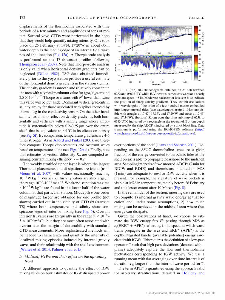
the water depth. Maximum crest to trough amplitude

frequently reach 40m or more over the outer shelf (see

Fig. 11). Short internal waves (wavelengths of a few

hundred meters) are embedded into longer waves

(wavelengths around 10km), as in situations where in-

ternal tides undergo fission (Gerkema 1996; Li and

Farmer 2011).

Beside visual resemblance between the patterns

exhibited in Fig. 11 and commonly observed internal

gravity waves, both yoyo CTDs and ScanFish observa-

tions at constant depth confirm that echograms reflect

FIG. 10. Across-shoreTSG temperature for five transects carried out

on 9 Mar 2013 over time intervals that are specified above each panel,

along with the exact latitude of the transect (148000 or 148050N). Note

the rapid changes in temperature distribution with time and latitude.



displacements of the thermocline associated with time

periods of a few minutes and amplitudes of tens of me-

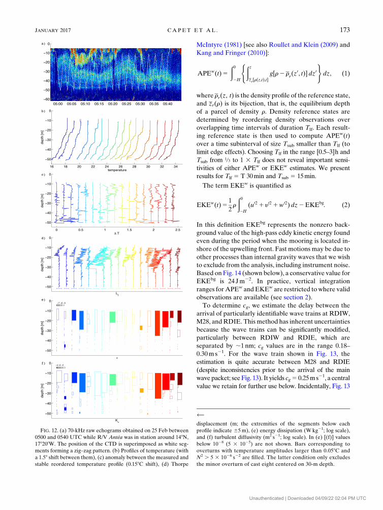
ters. Several yoyo CTDs were performed in the hope

that they would help quantifymixing intensity. One took

place on 25 February at 148N, 178200W in about 60-m

water depth as the leading edge of an internal tidal wave

passed that location (Fig. 12a). A Thorpe-scale analysis

is performed on the 17 downcast profiles, following

Thompson et al. (2007). Note that Thorpe-scale analysis

is only valid when horizontal density gradients can be

neglected (Dillon 1982). TSG data obtained immedi-

ately prior to the yoyo station provide a useful estimate

of the horizontal density gradients in the station vicinity.

The density gradient is smooth and relatively constant in

the areawith a typicalmaximumvalue for (g/r0)›xr around

2.53 1026 s22. Thorpe overturns withN2 lower than twice

this value will be put aside. Dominant vertical gradients in

salinity are by far those associated with spikes induced by

thermal lag in the conductivity sensor. On the other hand,

salinity has a minor effect on density gradients, both hori-

zontally and vertically with a salinity range whose ampli-

tude is systematically below 0.2–0.25 psu over the entire

shelf, that is, equivalent to ;18C in its effects on density

(see Fig. 5f). By comparison, temperature gradients are 4–5

times stronger. As in Alford and Pinkel (2000), we there-

fore compute Thorpe displacements and overturn scales

based on temperature alone (see Figs. 12b–d). Finally, note

that estimates of vertical diffusivity Ky are computed as-

suming constant mixing efficiency g 5 0.2.

The weakly stratified upper layer is where the largest

Thorpe displacements and dissipations are found (as in

Moum et al. 2007) with values occasionally reaching

1025Wkg21. Vertical diffusivity values are also large, in

the range 1023–1022m2 s21.Weaker dissipationmaxima

;1027Wkg21 are found in the lower half of the water

column at that particular station. Middepth « one order

of magnitude larger are obtained for one profile (not

shown) carried out in the vicinity of CTD 89 (transect

T8) where both temperature and salinity show con-

spicuous signs of interior mixing (see Fig. 6). Overall,

interior Ky values are frequently in the range 5 3 1025–

53 1023m2 s21, but they are most often associated with

overturns at the margin of detectability with standard

CTD measurements. More sophisticated methods will

be needed to characterize and quantify the intensity of

localized mixing episodes induced by internal gravity

waves and their relationship with the shelf environment

(Walter et al. 2014; Palmer et al. 2015).

b. Midshelf IGWs and their effect on the upwellingfront

A different approach to quantify the effect of IGW

mixing relies on bulk estimates of IGW dissipated power

over portions of the shelf (Jeans and Sherwin 2001). De-

pending on the SSUC thermohaline structure, a given

fraction of the energy converted to baroclinic tides at the

shelf break is able to propagate nearshore to the midshelf

area. Sampling intervals of twomooredADCPs (2min for

RDIW and RDIE) and thermistors mounted on M28

(1min) are adequate to resolve IGW activity when it is

present. For example, the signature of wave packets is

visible at M28 in temperature, mainly before 28 February

and to a lesser extent after 10 March (Fig. 8).

In the remainder of the section, mooring data are used

to compute 1) internal gravity wave energy at that lo-

cation and, under some assumptions, 2) how much

mixing can be achieved in the midshelf area where that

energy can dissipate.

Given the observations at hand, we choose to esti-

mate the IGW energy flux Fw passing through M28 as

cg(EKEw 1APEw), where cg is the speed at which wave

trains propagate in the area and EKEw (APEw) is the

depth-integrated kinetic (available potential) energy asso-

ciated with IGWs. This requires the definition of a low-pass

operator � such that high-pass deviations (denoted with a

prime) adequately capture the flow and thermohaline

fluctuations corresponding to IGW activity. We use a

running mean with flat averaging over time intervals of

duration Tlf longer than the internal wave period for � .The term APEw is quantified using the approach valid

for arbitrary stratifications detailed in Holliday and

FIG. 11. (top) 70-kHz echograms obtained on 23 Feb between

0222 and 0600 UTC while R/VAntéa steamed eastward at a nearly

constant speed;5 kt. Moderate backscatter levels in blue indicate

the position of sharp density gradients. They exhibit oscillations

with wavelengths of the order of a few hundred meters embedded

into longer internal tides (two wavelengths around 10 km are vis-

ible with troughs at 17.478, 17.378, and 17.298W and crests at 17.458and 17.348W). (bottom) Zoom over the time subinterval 0258 to

0343 UTC indicated by a rectangle in the top panel. Bottom depth

measured by the ship ADCP is indicated by a thick black line. Data

treatment is performed using the ECHOPEN software (http://

www.france-nord.ird.fr/les-ressources/outils-informatiques).



http://www.france-nord.ird.fr/les-ressources/outils-informatiques

http://www.france-nord.ird.fr/les-ressources/outils-informatiques

McIntyre (1981) [see also Roullet and Klein (2009) and

Kang and Fringer (2010)]:

APEw(t)5

ð02H

(ðzzr[r(z,t),t]

g[r2 rr(z0, t)] dz0

)dz, (1)

where rr(z, t) is the density profile of the reference state,

and zr(r) is its bijection, that is, the equilibrium depth

of a parcel of density r. Density reference states are

determined by reordering density observations over

overlapping time intervals of duration Tlf. Each result-

ing reference state is then used to compute APEw(t)

over a time subinterval of size Tsub smaller than Tlf (to

limit edge effects). Choosing Tlf in the range [0.5–3]h and

Tsub from 1/3 to 1 3 Tlf does not reveal important sensi-

tivities of either APEw or EKEw estimates. We present

results for Tlf 5 T 30min and Tsub 5 15min.

The term EKEw is quantified as

EKEw(t)51

2r

ð02H

(u02 1 y02 1w02) dz2EKEbg. (2)

In this definition EKEbg represents the nonzero back-

ground value of the high-pass eddy kinetic energy found

even during the period when the mooring is located in-

shore of the upwelling front. Fast motions may be due to

other processes than internal gravity waves that we wish

to exclude from the analysis, including instrument noise.

Based on Fig. 14 (shown below), a conservative value for

EKEbg is 24 Jm22. In practice, vertical integration

ranges for APEw andEKEw are restricted to where valid

observations are available (see section 2).

To determine cg, we estimate the delay between the

arrival of particularly identifiable wave trains at RDIW,

M28, andRDIE. This method has inherent uncertainties

because the wave trains can be significantly modified,

particularly between RDIW and RDIE, which are

separated by ;1nm; cg values are in the range 0.18–

0.30m s21. For the wave train shown in Fig. 13, the

estimation is quite accurate between M28 and RDIE

(despite inconsistencies prior to the arrival of the main

wave packet; see Fig. 13). It yields cg5 0.25ms21, a central

value we retain for further use below. Incidentally, Fig. 13

FIG. 12. (a) 70-kHz raw echograms obtained on 25 Feb between

0500 and 0540 UTC while R/V Antéa was in station around 148N,

178200W. The position of the CTD is superimposed as white seg-

ments forming a zig–zag pattern. (b) Profiles of temperature (with

a 1.58 shift between them), (c) anomaly between the measured and

stable reordered temperature profile (0.158C shift), (d) Thorpe

displacement (m; the extremities of the segments below each

profile indicate 65m), (e) energy dissipation (Wkg21; log scale),

and (f) turbulent diffusivity (m2 s21; log scale). In (e) [(f)] values

below 1028 (5 3 1025) are not shown. Bars corresponding to

overturns with temperature amplitudes larger than 0.058C and

N2 . 5 3 1026 s22 are filled. The latter condition only excludes

the minor overturn of cast eight centered on 30-m depth.



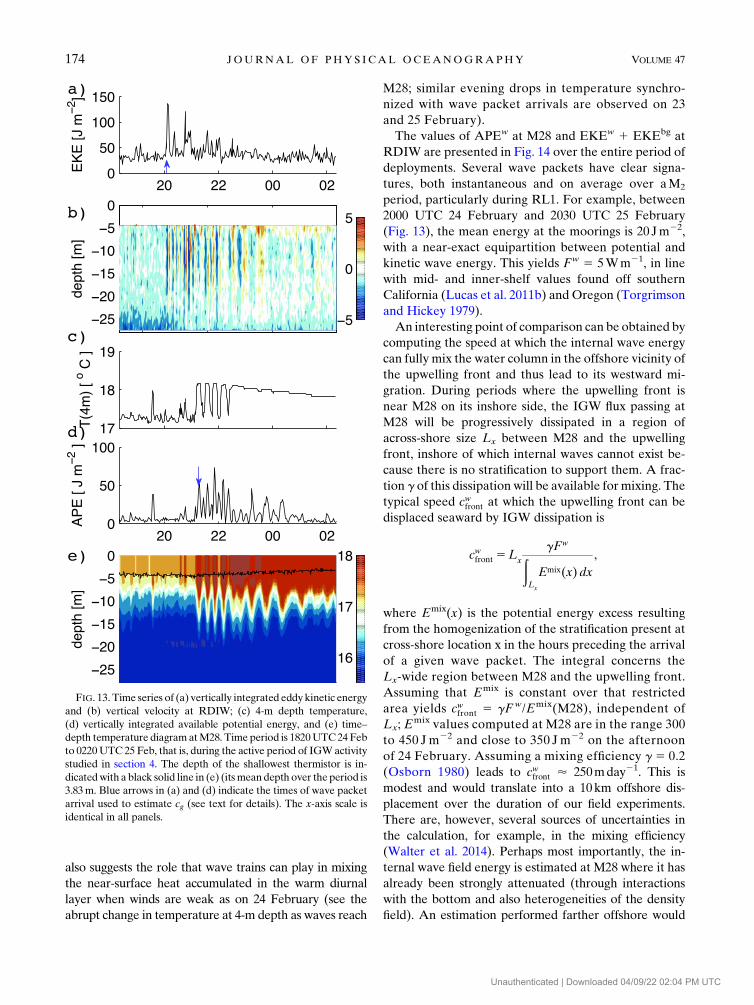
also suggests the role that wave trains can play in mixing

the near-surface heat accumulated in the warm diurnal

layer when winds are weak as on 24 February (see the

abrupt change in temperature at 4-m depth as waves reach

M28; similar evening drops in temperature synchro-

nized with wave packet arrivals are observed on 23

and 25 February).

The values of APEw at M28 and EKEw 1 EKEbg at

RDIW are presented in Fig. 14 over the entire period of

deployments. Several wave packets have clear signa-

tures, both instantaneous and on average over aM2

period, particularly during RL1. For example, between

2000 UTC 24 February and 2030 UTC 25 February

(Fig. 13), the mean energy at the moorings is 20 Jm22,

with a near-exact equipartition between potential and

kinetic wave energy. This yields Fw 5 5Wm21, in line

with mid- and inner-shelf values found off southern

California (Lucas et al. 2011b) and Oregon (Torgrimson

and Hickey 1979).

An interesting point of comparison can be obtained by

computing the speed at which the internal wave energy

can fully mix the water column in the offshore vicinity of

the upwelling front and thus lead to its westward mi-

gration. During periods where the upwelling front is

near M28 on its inshore side, the IGW flux passing at

M28 will be progressively dissipated in a region of

across-shore size Lx between M28 and the upwelling

front, inshore of which internal waves cannot exist be-

cause there is no stratification to support them. A frac-

tion g of this dissipation will be available for mixing. The

typical speed cwfront at which the upwelling front can be

displaced seaward by IGW dissipation is

cwfront 5Lx

gFwðLx

Emix(x) dx

,

where Emix(x) is the potential energy excess resulting

from the homogenization of the stratification present at

cross-shore location x in the hours preceding the arrival

of a given wave packet. The integral concerns the

Lx-wide region between M28 and the upwelling front.

Assuming that Emix is constant over that restricted

area yields cwfront 5 gF w/Emix(M28), independent of

Lx; Emix values computed at M28 are in the range 300

to 450 Jm22 and close to 350 Jm22 on the afternoon

of 24 February. Assuming a mixing efficiency g 5 0.2

(Osborn 1980) leads to cwfront ’ 250mday21. This is

modest and would translate into a 10km offshore dis-

placement over the duration of our field experiments.

There are, however, several sources of uncertainties in

the calculation, for example, in the mixing efficiency

(Walter et al. 2014). Perhaps most importantly, the in-

ternal wave field energy is estimated at M28 where it has

already been strongly attenuated (through interactions

with the bottom and also heterogeneities of the density

field). An estimation performed farther offshore would

FIG. 13. Time series of (a) vertically integrated eddykinetic energy

and (b) vertical velocity at RDIW; (c) 4-m depth temperature,

(d) vertically integrated available potential energy, and (e) time–

depth temperature diagramatM28. Time period is 1820UTC24 Feb

to 0220UTC 25 Feb, that is, during the active period of IGWactivity

studied in section 4. The depth of the shallowest thermistor is in-

dicatedwith a black solid line in (e) (itsmeandepth over the period is

3.83m. Blue arrows in (a) and (d) indicate the times of wave packet

arrival used to estimate cg (see text for details). The x-axis scale is

identical in all panels.



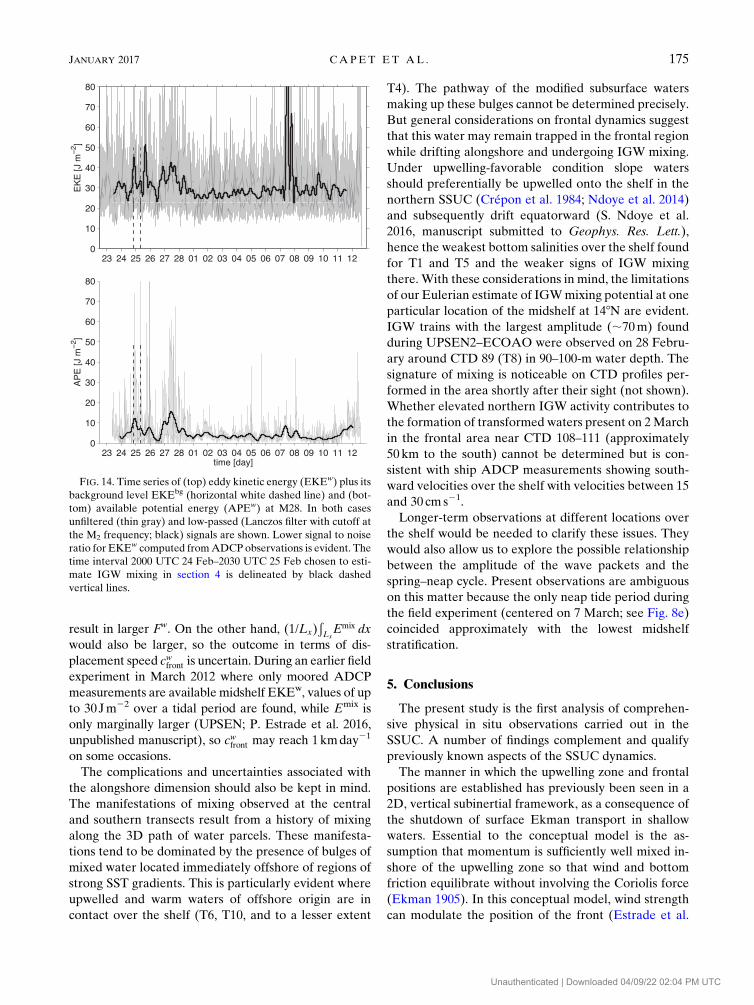
result in larger Fw. On the other hand, (1/Lx)ÐLxEmix dx

would also be larger, so the outcome in terms of dis-

placement speed cwfront is uncertain. During an earlier field

experiment in March 2012 where only moored ADCP

measurements are available midshelf EKEw, values of up

to 30Jm22 over a tidal period are found, while Emix is

only marginally larger (UPSEN; P. Estrade et al. 2016,

unpublished manuscript), so cwfront may reach 1kmday21

on some occasions.

The complications and uncertainties associated with

the alongshore dimension should also be kept in mind.

The manifestations of mixing observed at the central

and southern transects result from a history of mixing

along the 3D path of water parcels. These manifesta-

tions tend to be dominated by the presence of bulges of

mixed water located immediately offshore of regions of

strong SST gradients. This is particularly evident where

upwelled and warm waters of offshore origin are in

contact over the shelf (T6, T10, and to a lesser extent

T4). The pathway of the modified subsurface waters

making up these bulges cannot be determined precisely.

But general considerations on frontal dynamics suggest

that this water may remain trapped in the frontal region

while drifting alongshore and undergoing IGW mixing.

Under upwelling-favorable condition slope waters

should preferentially be upwelled onto the shelf in the

northern SSUC (Crépon et al. 1984; Ndoye et al. 2014)

and subsequently drift equatorward (S. Ndoye et al.

2016, manuscript submitted to Geophys. Res. Lett.),

hence the weakest bottom salinities over the shelf found

for T1 and T5 and the weaker signs of IGW mixing

there. With these considerations in mind, the limitations

of our Eulerian estimate of IGWmixing potential at one

particular location of the midshelf at 148N are evident.

IGW trains with the largest amplitude (;70m) found

during UPSEN2–ECOAO were observed on 28 Febru-

ary around CTD 89 (T8) in 90–100-m water depth. The

signature of mixing is noticeable on CTD profiles per-

formed in the area shortly after their sight (not shown).

Whether elevated northern IGW activity contributes to

the formation of transformed waters present on 2March

in the frontal area near CTD 108–111 (approximately

50 km to the south) cannot be determined but is con-

sistent with ship ADCP measurements showing south-

ward velocities over the shelf with velocities between 15

and 30 cm s21.

Longer-term observations at different locations over

the shelf would be needed to clarify these issues. They

would also allow us to explore the possible relationship

between the amplitude of the wave packets and the

spring–neap cycle. Present observations are ambiguous

on this matter because the only neap tide period during

the field experiment (centered on 7 March; see Fig. 8e)

coincided approximately with the lowest midshelf

stratification.

5. Conclusions

The present study is the first analysis of comprehen-

sive physical in situ observations carried out in the

SSUC. A number of findings complement and qualify

previously known aspects of the SSUC dynamics.

The manner in which the upwelling zone and frontal

positions are established has previously been seen in a

2D, vertical subinertial framework, as a consequence of

the shutdown of surface Ekman transport in shallow

waters. Essential to the conceptual model is the as-

sumption that momentum is sufficiently well mixed in-

shore of the upwelling zone so that wind and bottom

friction equilibrate without involving the Coriolis force

(Ekman 1905). In this conceptual model, wind strength

can modulate the position of the front (Estrade et al.

FIG. 14. Time series of (top) eddy kinetic energy (EKEw) plus its

background level EKEbg (horizontal white dashed line) and (bot-

tom) available potential energy (APEw) at M28. In both cases

unfiltered (thin gray) and low-passed (Lanczos filter with cutoff at

the M2 frequency; black) signals are shown. Lower signal to noise

ratio for EKEw computed fromADCPobservations is evident. The

time interval 2000 UTC 24 Feb–2030 UTC 25 Feb chosen to esti-

mate IGW mixing in section 4 is delineated by black dashed

vertical lines.



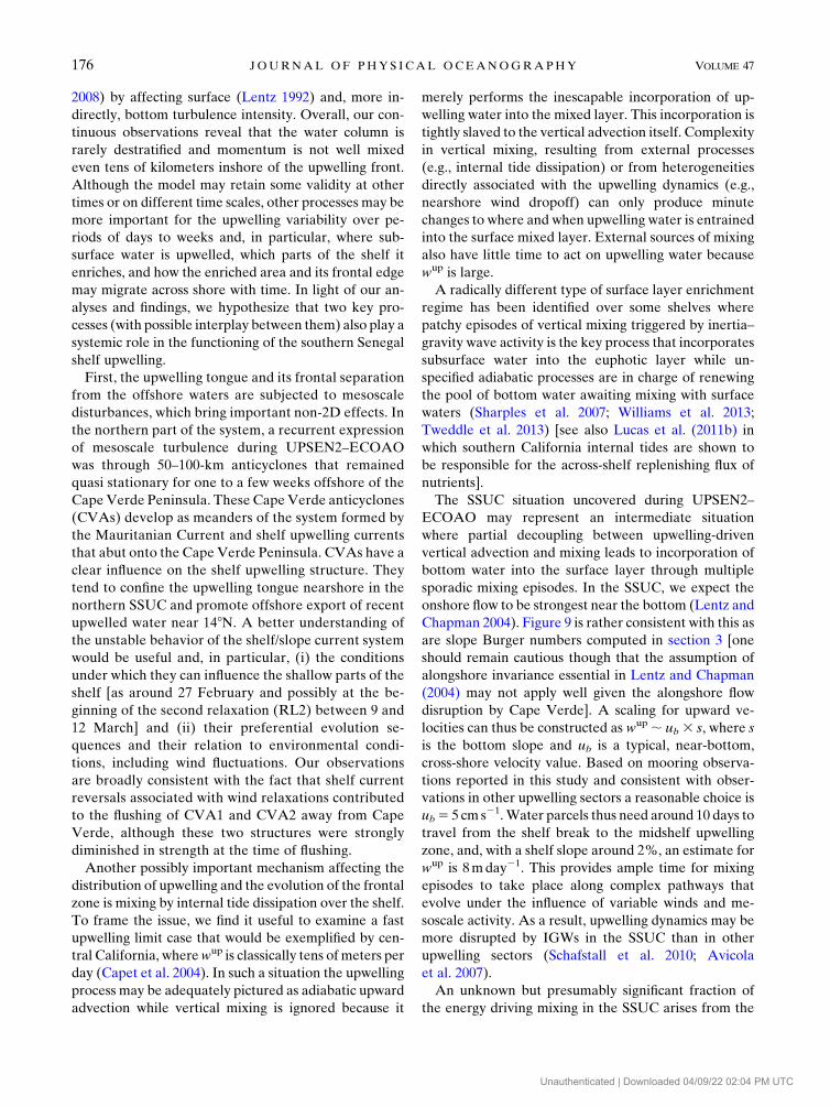
2008) by affecting surface (Lentz 1992) and, more in-

directly, bottom turbulence intensity. Overall, our con-

tinuous observations reveal that the water column is

rarely destratified and momentum is not well mixed

even tens of kilometers inshore of the upwelling front.

Although the model may retain some validity at other

times or on different time scales, other processes may be

more important for the upwelling variability over pe-

riods of days to weeks and, in particular, where sub-

surface water is upwelled, which parts of the shelf it

enriches, and how the enriched area and its frontal edge

may migrate across shore with time. In light of our an-

alyses and findings, we hypothesize that two key pro-

cesses (with possible interplay between them) also play a

systemic role in the functioning of the southern Senegal

shelf upwelling.

First, the upwelling tongue and its frontal separation

from the offshore waters are subjected to mesoscale

disturbances, which bring important non-2D effects. In

the northern part of the system, a recurrent expression

of mesoscale turbulence during UPSEN2–ECOAO

was through 50–100-km anticyclones that remained

quasi stationary for one to a few weeks offshore of the

CapeVerde Peninsula. These CapeVerde anticyclones

(CVAs) develop as meanders of the system formed by

the Mauritanian Current and shelf upwelling currents

that abut onto the Cape Verde Peninsula. CVAs have a

clear influence on the shelf upwelling structure. They

tend to confine the upwelling tongue nearshore in the

northern SSUC and promote offshore export of recent

upwelled water near 148N. A better understanding of

the unstable behavior of the shelf/slope current system

would be useful and, in particular, (i) the conditions

under which they can influence the shallow parts of the

shelf [as around 27 February and possibly at the be-

ginning of the second relaxation (RL2) between 9 and

12 March] and (ii) their preferential evolution se-

quences and their relation to environmental condi-

tions, including wind fluctuations. Our observations

are broadly consistent with the fact that shelf current

reversals associated with wind relaxations contributed

to the flushing of CVA1 and CVA2 away from Cape

Verde, although these two structures were strongly

diminished in strength at the time of flushing.

Another possibly important mechanism affecting the

distribution of upwelling and the evolution of the frontal

zone is mixing by internal tide dissipation over the shelf.

To frame the issue, we find it useful to examine a fast

upwelling limit case that would be exemplified by cen-

tral California, wherewup is classically tens of meters per

day (Capet et al. 2004). In such a situation the upwelling

process may be adequately pictured as adiabatic upward

advection while vertical mixing is ignored because it

merely performs the inescapable incorporation of up-

welling water into the mixed layer. This incorporation is

tightly slaved to the vertical advection itself. Complexity

in vertical mixing, resulting from external processes

(e.g., internal tide dissipation) or from heterogeneities

directly associated with the upwelling dynamics (e.g.,

nearshore wind dropoff) can only produce minute

changes to where and when upwelling water is entrained

into the surface mixed layer. External sources of mixing

also have little time to act on upwelling water because

wup is large.

A radically different type of surface layer enrichment

regime has been identified over some shelves where

patchy episodes of vertical mixing triggered by inertia–

gravity wave activity is the key process that incorporates

subsurface water into the euphotic layer while un-

specified adiabatic processes are in charge of renewing

the pool of bottom water awaiting mixing with surface

waters (Sharples et al. 2007; Williams et al. 2013;

Tweddle et al. 2013) [see also Lucas et al. (2011b) in

which southern California internal tides are shown to

be responsible for the across-shelf replenishing flux of

nutrients].

The SSUC situation uncovered during UPSEN2–

ECOAO may represent an intermediate situation

where partial decoupling between upwelling-driven

vertical advection and mixing leads to incorporation of

bottom water into the surface layer through multiple

sporadic mixing episodes. In the SSUC, we expect the

onshore flow to be strongest near the bottom (Lentz and

Chapman 2004). Figure 9 is rather consistent with this as

are slope Burger numbers computed in section 3 [one

should remain cautious though that the assumption of

alongshore invariance essential in Lentz and Chapman

(2004) may not apply well given the alongshore flow

disruption by Cape Verde]. A scaling for upward ve-

locities can thus be constructed as wup ; ub 3 s, where s

is the bottom slope and ub is a typical, near-bottom,

cross-shore velocity value. Based on mooring observa-

tions reported in this study and consistent with obser-

vations in other upwelling sectors a reasonable choice is

ub5 5 cm s21.Water parcels thus need around 10 days to

travel from the shelf break to the midshelf upwelling

zone, and, with a shelf slope around 2%, an estimate for

wup is 8mday21. This provides ample time for mixing

episodes to take place along complex pathways that

evolve under the influence of variable winds and me-

soscale activity. As a result, upwelling dynamics may be

more disrupted by IGWs in the SSUC than in other

upwelling sectors (Schafstall et al. 2010; Avicola

et al. 2007).

An unknown but presumably significant fraction of

the energy driving mixing in the SSUC arises from the



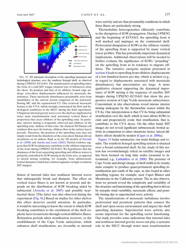
fission of internal tides into nonlinear internal waves

that subsequently break and dissipate. The effect on

vertical tracer fluxes is not known at present and de-

pends on the distribution of IGW breaking aided by

subinertial (Avicola et al. 2007) and possibly near-

inertial shear. [The latter was also observed during the

experiment (Fig. 9).] Based on studies for other shelves

this effect deserves careful attention. In particular,

it would be interesting to know the extent to which IGW

breaking contributes to the enrichment of the shelf eu-

photic layer in nutrients through vertical diffusive fluxes.

Relaxation periods when stratification recovers, or the

establishment of the Cape Verde anticyclone, which

enhances shelf stratification, are favorable to internal

wave activity and are thus presumably conditions in which

these fluxes are particularly strong.

Thermohaline heterogeneities efficiently contribute

to the disruption of IGW propagation. During UPSEN2

and the beginning of ECOAO, the upwelling front is

well marked and impinges on the continental shelf.

Preferential dissipation of IGWs in the offshore vicinity

of the upwelling front is supported by many vertical

tracer profiles. This has potentially important dynamical

implications. Additional observations will be needed to

further evaluate the significance of IGWs ‘‘pounding’’

on the upwelling front in its tendency to migrate off-

shore. The tentative energetic analysis presented in

section 4 leads to upwelling front offshore displacements

of a few hundred meters per day, which is modest (e.g.,

in regard to displacements associated with mesoscale

disturbances), but uncertainties are large. A more

qualitative element supporting the dynamical impor-

tance of IGW mixing is the sequence of satellite SST

images during UPSEN2–ECOAO that show the pro-

gressive erosion of Cape Verde mesoscale anticyclones.

Concomitant in situ observations reveal intense interior

mixing undergone by the thermocline waters within the

CVAs. Our interpretation is that CVAs bring substantial

stratification over the shelf, which in turn allows IGWs to

exist and progressively erode that stratification, that is,

contribute to the CVA decay. On the other hand, SST

images do not reveal significant submesoscale frontal ac-

tivity in comparison to other situations; hence, lateral dif-

fusive effects should be modest (Capet et al. 2008a).

Figure 15 helps summarize our main findings and re-

sults. The southern Senegal upwelling system is situated

over a broad continental shelf. So far, study of this sys-

tem has overwhelmingly relied on satellite images and

has been focused on long time scales (seasonal to in-

terannual; e.g., Lathuilière et al. 2008). The presence of

CapeVerde and abrupt change of shelf width in its vicinity

must conspire to produce quasi-permanent upwelling in-

tensification just south of the cape, as also found in other

upwelling regions, for example, near Capes Blanco and

Mendocino in the California system. The in situ observa-

tions we present reveal the complexity and variability of

the structure and functioning of the upwelling that is driven

by synoptic wind variability, mesoscale effects, and possi-

bly mixing due to superinertial wave activity.

The manifestations of mesoscale turbulence involve

preferential and persistent patterns that connect the

shelf and open-ocean environment and impact the shelf

upwelling dynamics. Superinertial wave activity also

seems important for the upwelling sector functioning.

Our study provides some indications that internal tides

and nonlinear internal gravity waves can play a systemic

role in the SSUC through water mass transformation

FIG. 15. 3D schematic description of the upwelling dynamical and

hydrological structure over the southern Senegal shelf, as observed

during UPSEN2–ECOAO. The manifestation of upwelling takes

the form of a cold SST tongue situated tens of kilometers away

the shore. Its position and that of its offshore frontal edge un-

dergo cross-shore displacements influenced by mesoscale dis-

turbances. These mesoscale disturbances presumably arise from

instabilities of the current system composed of the poleward-

flowing MC and the equatorward UJ. One recurrent mesoscale

feature is the CVA, which strongly constrained the flow and hy-

drological conditions in the SSUC during the field experiment.

Ubiquitous internal gravity waves over the shelf are implicated in

water mass transformation (and associated vertical fluxes of

properties) that occur offshore of the upwelling zone. In partic-

ular, interior mixing is frequently observed just offshore of the

upwelling zone. Inshore of that zone, the classical 2D Ekman cell

(onshore flow near the bottom, offshore flow in the surface layer)

prevails. Therefore, the position of the upwelling zone may not

simply result from the shutdown of the cross-shore Ekman-driven

circulation on its inshore flank as in the 2D models of Estrade

et al. (2008) and Austin and Lentz (2002). Partial evidence sug-

gests that IGWbreakingmay contribute to the offshoremigration

of the front during UPSEN2–ECOAO. We hypothesize that the

sharpness of the front separating upwelling and offshore waters is

primarily controlled by IGWmixing in the front area, as opposed

to lateral mixing resulting, for example, from submesoscale

frontal dynamics (which has a limited signature in high-resolution

SST images).



and vertical flux of properties. In sustained upwelling

conditions, where most of the subsurface water feeding

the coastal divergence enters the shelf area in the

northern SSUC and subsequently flows southward (S.

Ndoye et al. 2016, manuscript submitted to Geophys.

Res. Lett.), we expect the stratification to be increasingly

impacted by IGWs toward the south (i.e., downstream

with respect to the dominant shelf circulation), as we

generally observe during UPSEN2–ECOAO. However,

water residence time scales over the southern Senegal

shelf are comparable to those of synoptic variability.

Water property modifications and biogeochemical

activity thus take place along complex pathways that

integrate the influence of synoptic wind variability and

mesoscale and internal tide activity. How much of that

complexity needs to be accounted for to properly un-

derstand the ecological functioning of the SSUC (e.g.,

as a nursery for small pelagic fish) and its long-term

evolution will be the subject of future research. Most

urgently perhaps, the conditions in which very low

dissolved oxygen levels develop over the shelf, as

during the final part of UPSEN2–ECOAO experi-

ments, need to be clarified.

Acknowledgments.We are grateful to the captain and

crew of R/V Antéa for their dedication and pro-

fessionalism. We acknowledge financial support from

IRD through the AWA and LMI ECLAIRS programs,

from LEFE-INSU FUSE, and from European Union

FP7 PREFACE. S.N. was supported by the Programme

doctoral international modélisation des systèmes com-

plexes UPMC/IRD. Much assistance was provided by

Unité de Service IMAGO (IRD, Plouzané), including on

land support with satellite imagery by D. Dagorne. We

thank B. Le Cann and C. Roy for helpful discussions and

two anonymous reviewers for their insightful and con-

structive comments on the manuscript. Level 2 SST

MODIS and ASCAT data were downloaded fromNASA

(http://oceancolor.gsfc.nasa.gov/). QuikSCAT data were

downloaded online (at ftp://podaac-ftp.jpl.nasa.gov/allData/

ascat/preview/L2/). Wind data from Dakar weather

station were downloaded online (at www.ogimet.com/

metars.phtml.en).

REFERENCES

Adams,K.A., J.A.Barth, andF.Chan, 2013: Temporal variability of

near-bottom dissolved oxygen during upwelling off central

Oregon. J. Geophys. Res. Oceans, 118, 4839–4854, doi:10.1002/

jgrc.20361.

Alford, M. H., and R. Pinkel, 2000: Observations of overturning in

the thermocline: The context of ocean mixing. J. Phys. Oce-

anogr., 30, 805–832, doi:10.1175/1520-0485(2000)030,0805:

OOOITT.2.0.CO;2.

Allen, J., P. Newberger, and J. Federiuk, 1995: Upwelling circula-

tion on the Oregon continental shelf. Part I: Response to

idealized forcing. J. Phys. Oceanogr., 25, 1843–1866, doi:10.1175/

1520-0485(1995)025,1843:UCOTOC.2.0.CO;2.

Aristegui, J., and Coauthors, 2009: Sub-regional ecosystem vari-

ability in the canary current upwelling. Prog. Oceanogr., 83,

33–48, doi:10.1016/j.pocean.2009.07.031.

Austin, J. A., and J. A. Barth, 2002: Variation in the position of the

upwelling front on the Oregon shelf. J. Geophys. Res., 107,

3180, doi:10.1029/2001JC000858.

——, and S. J. Lentz, 2002: The inner shelf response to wind-driven

upwelling and downwelling. J. Phys. Oceanogr., 32, 2171–2193,

doi:10.1175/1520-0485(2002)032,2171:TISRTW.2.0.CO;2.

Avicola, G., J. N. Moum, A. Perlin, and M. D. Levine, 2007: En-

hanced turbulence due to the superposition of internal gravity

waves and a coastal upwelling jet. J. Geophys. Res., 112,

C06024, doi:10.1029/2006JC003831.

Barton, E. D., 1989: The poleward undercurrent on the eastern

boundary of the subtropical North Atlantic. Poleward Flows

Along Eastern Ocean Boundaries, S. J. Neshyba et al., Eds.,

Springer, 82–95.

——, 1998: Eastern boundary of the North Atlantic: Northwest

Africa and Iberia. The Global Coastal Ocean: Regional

Studies and Syntheses, A. R. Robinson and K. H. Brink,

Eds., The Sea—Ideas and Observations on Progress in

the Study of the Seas, Vol. 11, John Wiley and Sons,

633–657.

——, A. Huyer, and R. L. Smith, 1977: Temporal variation ob-

served in the hydrographic regime near Cabo Corveiro in the

northwest African upwelling region, February to April 1974.

Deep-Sea Res., 24, 7–23, doi:10.1016/0146-6291(77)90537-9.

Boccaletti, G., R. Ferrari, and B. Fox-Kemper, 2007: Mixed layer

instabilities and restratification. J. Phys. Oceanogr., 37, 2228–

2250, doi:10.1175/JPO3101.1.

Bretherton, F. P., R. E.Davis, andC. Fandry, 1976: A technique for

objective analysis and design of oceanographic experiments

applied to MODE-73. Deep-Sea Res. Oceanogr. Abstr., 23,

559–582, doi:10.1016/0011-7471(76)90001-2.

Capet, X., P. Marchesiello, and J. C. McWilliams, 2004: Upwelling

response to coastal wind profiles. Geophys. Res. Lett., 31,

L13311, doi:10.1029/2004GL020123.

——, E. J. Campos, and A. M. Paiva, 2008a: Submesoscale activity

over the Argentinian shelf. Geophys. Res. Lett., 35, L15605,

doi:10.1029/2008GL034736.

——, F. Colas, P. Penven, P. Marchesiello, and J. C. McWilliams,

2008b: Eddies in eastern boundary subtropical upwelling sys-

tems. Ocean Modeling in an Eddying Regime, Geophys.

Monogr., Vol. 177, Amer. Geophys. Union, 131–147.

——, J. C. McWilliams, M. J. Molemaker, and A. Shchepetkin,

2008c: Mesoscale to submesoscale transition in the California

Current System. Part I: Flow structure and eddy flux. J. Phys.

Oceanogr., 38, 29–43, doi:10.1175/2007JPO3671.1.

——, ——, ——, and ——, 2008d: Mesoscale to submesoscale tran-

sition in theCalifornia Current System. Part II: Frontal processes.

J. Phys. Oceanogr., 38, 44–64, doi:10.1175/2007JPO3672.1.

Citeau, J., L. Finaud, J. Cammas, and H. Demarcq, 1989:

Questions relative to ITCZ migrations over the tropical

Atlantic Ocean, sea surface temperature and Senegal River

runoff. Meteor. Atmos. Phys., 41, 181–190, doi:10.1007/

BF01026109.

Crépon, M., C. Richez, and M. Chartier, 1984: Effects of coastline

geometry on upwellings. J. Phys. Oceanogr., 14, 1365–1382,

doi:10.1175/1520-0485(1984)014,1365:EOCGOU.2.0.CO;2.



http://oceancolor.gsfc.nasa.gov/

ftp://podaac-ftp.jpl.nasa.gov/allData/ascat/preview/L2/

ftp://podaac-ftp.jpl.nasa.gov/allData/ascat/preview/L2/



http://dx.doi.org/10.1002/jgrc.20361

http://dx.doi.org/10.1002/jgrc.20361

http://dx.doi.org/10.1175/1520-0485(2000)030<0805:OOOITT>2.0.CO;2

http://dx.doi.org/10.1175/1520-0485(2000)030<0805:OOOITT>2.0.CO;2

http://dx.doi.org/10.1175/1520-0485(1995)025<1843:UCOTOC>2.0.CO;2

http://dx.doi.org/10.1175/1520-0485(1995)025<1843:UCOTOC>2.0.CO;2

http://dx.doi.org/10.1016/j.pocean.2009.07.031

http://dx.doi.org/10.1029/2001JC000858

http://dx.doi.org/10.1175/1520-0485(2002)032<2171:TISRTW>2.0.CO;2

http://dx.doi.org/10.1029/2006JC003831

http://dx.doi.org/10.1016/0146-6291(77)90537-9

http://dx.doi.org/10.1175/JPO3101.1

http://dx.doi.org/10.1016/0011-7471(76)90001-2

http://dx.doi.org/10.1029/2004GL020123

http://dx.doi.org/10.1029/2008GL034736

http://dx.doi.org/10.1175/2007JPO3671.1


http://dx.doi.org/10.1007/BF01026109

http://dx.doi.org/10.1007/BF01026109

http://dx.doi.org/10.1175/1520-0485(1984)014<1365:EOCGOU>2.0.CO;2

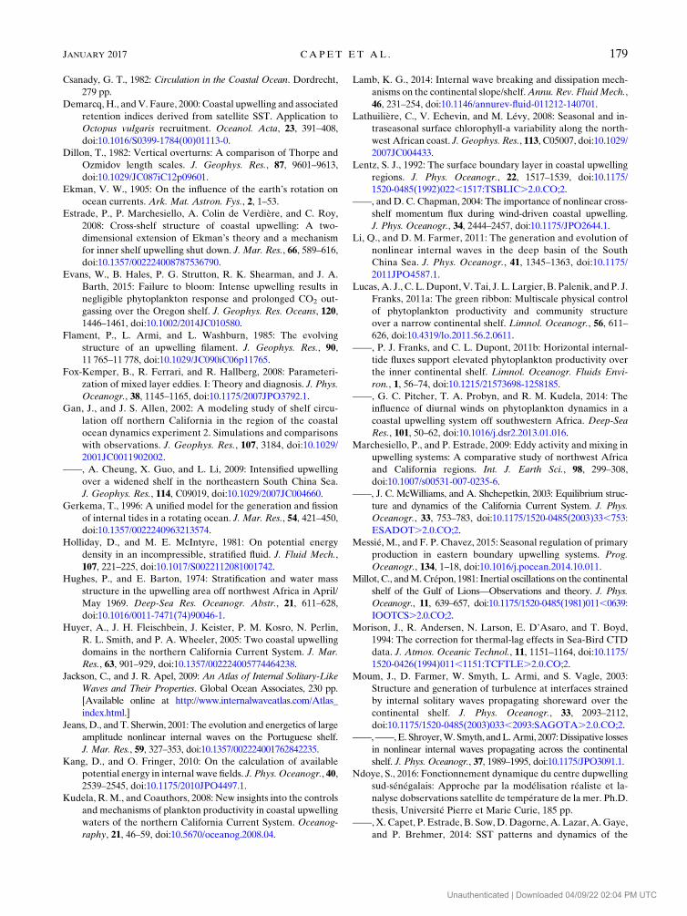
Csanady, G. T., 1982: Circulation in the Coastal Ocean. Dordrecht,

279 pp.

Demarcq, H., andV. Faure, 2000: Coastal upwelling and associated

retention indices derived from satellite SST. Application to

Octopus vulgaris recruitment. Oceanol. Acta, 23, 391–408,

doi:10.1016/S0399-1784(00)01113-0.

Dillon, T., 1982: Vertical overturns: A comparison of Thorpe and

Ozmidov length scales. J. Geophys. Res., 87, 9601–9613,

doi:10.1029/JC087iC12p09601.

Ekman, V. W., 1905: On the influence of the earth’s rotation on

ocean currents. Ark. Mat. Astron. Fys., 2, 1–53.Estrade, P., P. Marchesiello, A. Colin de Verdière, and C. Roy,

2008: Cross-shelf structure of coastal upwelling: A two-

dimensional extension of Ekman’s theory and a mechanism

for inner shelf upwelling shut down. J. Mar. Res., 66, 589–616,

doi:10.1357/002224008787536790.

Evans, W., B. Hales, P. G. Strutton, R. K. Shearman, and J. A.

Barth, 2015: Failure to bloom: Intense upwelling results in

negligible phytoplankton response and prolonged CO2 out-

gassing over the Oregon shelf. J. Geophys. Res. Oceans, 120,

1446–1461, doi:10.1002/2014JC010580.

Flament, P., L. Armi, and L. Washburn, 1985: The evolving

structure of an upwelling filament. J. Geophys. Res., 90,

11 765–11 778, doi:10.1029/JC090iC06p11765.

Fox-Kemper, B., R. Ferrari, and R. Hallberg, 2008: Parameteri-

zation of mixed layer eddies. I: Theory and diagnosis. J. Phys.

Oceanogr., 38, 1145–1165, doi:10.1175/2007JPO3792.1.

Gan, J., and J. S. Allen, 2002: A modeling study of shelf circu-

lation off northern California in the region of the coastal

ocean dynamics experiment 2. Simulations and comparisons

with observations. J. Geophys. Res., 107, 3184, doi:10.1029/

2001JC0011902002.

——, A. Cheung, X. Guo, and L. Li, 2009: Intensified upwelling

over a widened shelf in the northeastern South China Sea.

J. Geophys. Res., 114, C09019, doi:10.1029/2007JC004660.

Gerkema, T., 1996: A unified model for the generation and fission

of internal tides in a rotating ocean. J. Mar. Res., 54, 421–450,

doi:10.1357/0022240963213574.

Holliday, D., and M. E. McIntyre, 1981: On potential energy

density in an incompressible, stratified fluid. J. Fluid Mech.,

107, 221–225, doi:10.1017/S0022112081001742.Hughes, P., and E. Barton, 1974: Stratification and water mass

structure in the upwelling area off northwest Africa in April/

May 1969. Deep-Sea Res. Oceanogr. Abstr., 21, 611–628,

doi:10.1016/0011-7471(74)90046-1.

Huyer, A., J. H. Fleischbein, J. Keister, P. M. Kosro, N. Perlin,

R. L. Smith, and P. A. Wheeler, 2005: Two coastal upwelling

domains in the northern California Current System. J. Mar.

Res., 63, 901–929, doi:10.1357/002224005774464238.

Jackson, C., and J. R. Apel, 2009: An Atlas of Internal Solitary-Like

Waves and Their Properties. Global Ocean Associates, 230 pp.

[Available online at http://www.internalwaveatlas.com/Atlas_

index.html.]

Jeans, D., and T. Sherwin, 2001: The evolution and energetics of large

amplitude nonlinear internal waves on the Portuguese shelf.

J. Mar. Res., 59, 327–353, doi:10.1357/002224001762842235.

Kang, D., and O. Fringer, 2010: On the calculation of available

potential energy in internal wave fields. J. Phys. Oceanogr., 40,

2539–2545, doi:10.1175/2010JPO4497.1.

Kudela, R. M., and Coauthors, 2008: New insights into the controls

and mechanisms of plankton productivity in coastal upwelling

waters of the northern California Current System. Oceanog-

raphy, 21, 46–59, doi:10.5670/oceanog.2008.04.

Lamb, K. G., 2014: Internal wave breaking and dissipation mech-

anisms on the continental slope/shelf.Annu. Rev. FluidMech.,

46, 231–254, doi:10.1146/annurev-fluid-011212-140701.

Lathuilière, C., V. Echevin, and M. Lévy, 2008: Seasonal and in-

traseasonal surface chlorophyll-a variability along the north-

west African coast. J. Geophys. Res., 113, C05007, doi:10.1029/

2007JC004433.

Lentz, S. J., 1992: The surface boundary layer in coastal upwelling

regions. J. Phys. Oceanogr., 22, 1517–1539, doi:10.1175/

1520-0485(1992)022,1517:TSBLIC.2.0.CO;2.

——, and D. C. Chapman, 2004: The importance of nonlinear cross-

shelf momentum flux during wind-driven coastal upwelling.

J. Phys. Oceanogr., 34, 2444–2457, doi:10.1175/JPO2644.1.

Li, Q., and D. M. Farmer, 2011: The generation and evolution of

nonlinear internal waves in the deep basin of the South

China Sea. J. Phys. Oceanogr., 41, 1345–1363, doi:10.1175/

2011JPO4587.1.

Lucas, A. J., C. L.Dupont, V. Tai, J. L. Largier, B. Palenik, and P. J.

Franks, 2011a: The green ribbon: Multiscale physical control

of phytoplankton productivity and community structure

over a narrow continental shelf. Limnol. Oceanogr., 56, 611–

626, doi:10.4319/lo.2011.56.2.0611.

——, P. J. Franks, and C. L. Dupont, 2011b: Horizontal internal-

tide fluxes support elevated phytoplankton productivity over

the inner continental shelf. Limnol. Oceanogr. Fluids Envi-

ron., 1, 56–74, doi:10.1215/21573698-1258185.

——, G. C. Pitcher, T. A. Probyn, and R. M. Kudela, 2014: The

influence of diurnal winds on phytoplankton dynamics in a

coastal upwelling system off southwestern Africa. Deep-Sea

Res., 101, 50–62, doi:10.1016/j.dsr2.2013.01.016.

Marchesiello, P., and P. Estrade, 2009: Eddy activity and mixing in

upwelling systems: A comparative study of northwest Africa

and California regions. Int. J. Earth Sci., 98, 299–308,

doi:10.1007/s00531-007-0235-6.

——, J. C. McWilliams, and A. Shchepetkin, 2003: Equilibrium struc-

ture and dynamics of the California Current System. J. Phys.

Oceanogr., 33, 753–783, doi:10.1175/1520-0485(2003)33,753:

ESADOT.2.0.CO;2.

Messié, M., and F. P. Chavez, 2015: Seasonal regulation of primary

production in eastern boundary upwelling systems. Prog.

Oceanogr., 134, 1–18, doi:10.1016/j.pocean.2014.10.011.

Millot, C., andM.Crépon, 1981: Inertial oscillations on the continentalshelf of the Gulf of Lions—Observations and theory. J. Phys.

Oceanogr., 11, 639–657, doi:10.1175/1520-0485(1981)011,0639:

IOOTCS.2.0.CO;2.

Morison, J., R. Andersen, N. Larson, E. D’Asaro, and T. Boyd,

1994: The correction for thermal-lag effects in Sea-Bird CTD

data. J. Atmos. Oceanic Technol., 11, 1151–1164, doi:10.1175/

1520-0426(1994)011,1151:TCFTLE.2.0.CO;2.

Moum, J., D. Farmer, W. Smyth, L. Armi, and S. Vagle, 2003:

Structure and generation of turbulence at interfaces strained

by internal solitary waves propagating shoreward over the

continental shelf. J. Phys. Oceanogr., 33, 2093–2112,

doi:10.1175/1520-0485(2003)033,2093:SAGOTA.2.0.CO;2.

——,——,E. Shroyer,W. Smyth, andL.Armi, 2007:Dissipative losses

in nonlinear internal waves propagating across the continental

shelf. J. Phys. Oceanogr., 37, 1989–1995, doi:10.1175/JPO3091.1.

Ndoye, S., 2016: Fonctionnement dynamique du centre dupwelling

sud-sénégalais: Approche par la modélisation réaliste et la-

nalyse dobservations satellite de température de la mer. Ph.D.

thesis, Université Pierre et Marie Curie, 185 pp.

——,X. Capet, P. Estrade, B. Sow,D.Dagorne,A. Lazar, A.Gaye,

and P. Brehmer, 2014: SST patterns and dynamics of the



http://dx.doi.org/10.1016/S0399-1784(00)01113-0

http://dx.doi.org/10.1029/JC087iC12p09601

http://dx.doi.org/10.1357/002224008787536790

http://dx.doi.org/10.1002/2014JC010580

http://dx.doi.org/10.1029/JC090iC06p11765


http://dx.doi.org/10.1029/2001JC0011902002

http://dx.doi.org/10.1029/2001JC0011902002

http://dx.doi.org/10.1029/2007JC004660

http://dx.doi.org/10.1357/0022240963213574

http://dx.doi.org/10.1017/S0022112081001742

http://dx.doi.org/10.1016/0011-7471(74)90046-1

http://dx.doi.org/10.1357/002224005774464238

http://www.internalwaveatlas.com/Atlas_index.html

http://www.internalwaveatlas.com/Atlas_index.html

http://dx.doi.org/10.1357/002224001762842235


http://dx.doi.org/10.5670/oceanog.2008.04

http://dx.doi.org/10.1146/annurev-fluid-011212-140701

http://dx.doi.org/10.1029/2007JC004433

http://dx.doi.org/10.1029/2007JC004433

http://dx.doi.org/10.1175/1520-0485(1992)022<1517:TSBLIC>2.0.CO;2

http://dx.doi.org/10.1175/1520-0485(1992)022<1517:TSBLIC>2.0.CO;2




http://dx.doi.org/10.4319/lo.2011.56.2.0611

http://dx.doi.org/10.1215/21573698-1258185

http://dx.doi.org/10.1016/j.dsr2.2013.01.016

http://dx.doi.org/10.1007/s00531-007-0235-6

http://dx.doi.org/10.1175/1520-0485(2003)33<753:ESADOT>2.0.CO;2

http://dx.doi.org/10.1175/1520-0485(2003)33<753:ESADOT>2.0.CO;2


http://dx.doi.org/10.1175/1520-0485(1981)011<0639:IOOTCS>2.0.CO;2

http://dx.doi.org/10.1175/1520-0485(1981)011<0639:IOOTCS>2.0.CO;2

http://dx.doi.org/10.1175/1520-0426(1994)011<1151:TCFTLE>2.0.CO;2

http://dx.doi.org/10.1175/1520-0426(1994)011<1151:TCFTLE>2.0.CO;2

http://dx.doi.org/10.1175/1520-0485(2003)033<2093:SAGOTA>2.0.CO;2


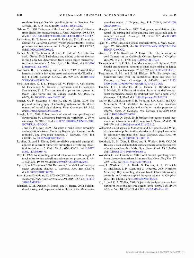
southern Senegal-Gambia upwelling center. J. Geophys. Res.

Oceans, 119, 8315–8335, doi:10.1002/2014JC010242.

Osborn, T., 1980: Estimates of the local rate of vertical diffusion

from dissipation measurements. J. Phys. Oceanogr., 10, 83–89,doi:10.1175/1520-0485(1980)010,0083:EOTLRO.2.0.CO;2.

Pallàs-Sanz, E., T. Johnston, and D. Rudnick, 2010: Frontal dy-

namics in a California Current System shallow front: 1. Frontal

processes and tracer structure. J. Geophys. Res., 115, C12067,doi:10.1029/2009JC006032.

Palmer, M., G. Stephenson, M. Inall, C. Balfour, A. Düsterhus,and J. Green, 2015: Turbulence and mixing by internal waves

in the Celtic Sea determined from ocean glider microstruc-

ture measurements. J. Mar. Syst., 144, 57–69, doi:10.1016/

j.jmarsys.2014.11.005.

Pawlowicz, R., B. Beardsley, and S. Lentz, 2002: Classical tidal

harmonic analysis including error estimates in MATLAB us-

ing T_TIDE. Comput. Geosci., 28, 929–937, doi:10.1016/

S0098-3004(02)00013-4.

Peña-Izquierdo, J., J. L. Pelegrí, M. V. Pastor, P. Castellanos,

M. Emelianov, M. Gasser, J. Salvador, and E. Vázquez-Domínguez, 2012: The continental slope current system be-

tween Cape Verde and the Canary Islands. Sci. Mar., 76,

65–78, doi:10.3989/scimar.03607.18C.

Pitcher, G., F. Figueiras, B. Hickey, and M. Moita, 2010: The

physical oceanography of upwelling systems and the devel-

opment of harmful algal blooms. Prog. Oceanogr., 85, 5–32,doi:10.1016/j.pocean.2010.02.002.

Pringle, J. M., 2002: Enhancement of wind-driven upwelling and

downwelling by alongshore bathymetric variability. J. Phys.

Oceanogr., 32, 3101–3112, doi:10.1175/1520-0485(2002)032,3101:

EOWDUA.2.0.CO;2.

——, and E. P. Dever, 2009: Dynamics of wind-driven upwelling

and relaxation betweenMonterey Bay and point arena: Local-,

regional-, and gyre-scale controls. J. Geophys. Res., 114,C07003, doi:10.1029/2008JC005016.

Roullet, G., and P. Klein, 2009: Available potential energy di-

agnosis in a direct numerical simulation of rotating strati-

fied turbulence. J. Fluid Mech., 624, 45–55, doi:10.1017/

S0022112008004473.

Roy, C., 1998: An upwelling-induced retention area off Senegal: A

mechanism to link upwelling and retention processes. S. Afr.

J. Mar. Sci., 19, 89–98, doi:10.2989/025776198784126881.

Ryan, J., and Coauthors, 2010: Recurrent frontal slicks of a coastal

ocean upwelling shadow. J. Geophys. Res., 115, C12070,

doi:10.1029/2010JC006398.

Saha, S., and Coauthors, 2010: TheNCEPClimate Forecast System

Reanalysis.Bull. Amer.Meteor. Soc., 91, 1015–1057, doi:10.1175/

2010BAMS3001.1.

Schafstall, J., M. Dengler, P. Brandt, and H. Bange, 2010: Tidal-in-

duced mixing and diapycnal nutrient fluxes in the Mauritanian

upwelling region. J. Geophys. Res., 115, C10014, doi:10.1029/

2009JC005940.

Sharples, J., and Coauthors, 2007: Spring-neap modulation of in-

ternal tide mixing and vertical nitrate fluxes at a shelf edge in

summer. Limnol. Oceanogr., 52, 1735–1747, doi:10.4319/

lo.2007.52.5.1735.

Spall, M., 1997: Baroclinic jets in confluent flows. J. Phys. Ocean-

ogr., 27, 1054–1071, doi:10.1175/1520-0485(1997)027,1054:

BJICF.2.0.CO;2.

Strub, P. T., P. M. Kosro, and A. Huyer, 1991: The nature of the

cold filaments in the California Current System. J. Geophys.

Res., 96, 14 743–14 768, doi:10.1029/91JC01024.Thompson, A. F., S. T. Gille, J. A. MacKinnon, and J. Sprintall, 2007:

Spatial and temporal patterns of small-scale mixing in Drake

Passage. J. Phys.Oceanogr., 37, 572–592, doi:10.1175/JPO3021.1.

Torgrimson, G. M., and B. M. Hickey, 1979: Barotropic and

baroclinic tides over the continental slope and shelf off

Oregon. J. Phys. Oceanogr., 9, 945–961, doi:10.1175/

1520-0485(1979)009,0945:BABTOT.2.0.CO;2.

Tweddle, J. F., J. Sharples, M. R. Palmer, K. Davidson, and

S. McNeill, 2013: Enhanced nutrient fluxes at the shelf sea sea-

sonal thermocline caused by stratified flow over a bank. Prog.

Oceanogr., 117, 37–47, doi:10.1016/j.pocean.2013.06.018.Walter, R. K., M. E. Squibb, C. B.Woodson, J. R. Koseff, and S. G.

Monismith, 2014: Stratified turbulence in the nearshore

coastal ocean: Dynamics and evolution in the presence of

internal bores. J. Geophys. Res. Oceans, 119, 8709–8730,

doi:10.1002/2014JC010396.

Wang, D.-P., and A. Jordi, 2011: Surface frontogenesis and ther-

mohaline intrusion in a shelfbreak front. Ocean Modell., 38,161–170, doi:10.1016/j.ocemod.2011.02.012.

Williams, C., J. Sharples, C.Mahaffey, and T. Rippeth, 2013:Wind-

driven nutrient pulses to the subsurface chlorophyll maximum

in seasonally stratified shelf seas. Geophys. Res. Lett., 40,5467–5472, doi:10.1002/2013GL058171.

Woodruff, S., H. Diaz, J. Elms, and S. Worley, 1998: COADS

Release 2 data andmetadata enhancements for improvements

of marine surface flux fields. Phys. Chem. Earth, 23, 517–526,

doi:10.1016/S0079-1946(98)00064-0.

Woodson, C., and Coauthors, 2007: Local diurnal upwelling driven

by sea breezes in northernMonterey Bay.Cont. Shelf Res., 27,2289–2302, doi:10.1016/j.csr.2007.05.014.

——, L. Washburn, J. A. Barth, D. Hoover, A. R. Kirincich,

M. McManus, J. P. Ryan, and J. Tyburczy, 2009: Northern

Monterey Bay upwelling shadow front: Observations of a

coastally and surface-trapped buoyant plume. J. Geophys.

Res., 114, C12013, doi:10.1029/2009JC005623.

Yu, L., and R. A. Weller, 2007: Objectively analyzed air–sea heat

fluxes for the global ice-free oceans (1981–2005). Bull. Amer.

Meteor. Soc., 88, 527–539, doi:10.1175/BAMS-88-4-527.



http://dx.doi.org/10.1002/2014JC010242

http://dx.doi.org/10.1175/1520-0485(1980)010<0083:EOTLRO>2.0.CO;2

http://dx.doi.org/10.1029/2009JC006032

http://dx.doi.org/10.1016/j.jmarsys.2014.11.005

http://dx.doi.org/10.1016/j.jmarsys.2014.11.005

http://dx.doi.org/10.1016/S0098-3004(02)00013-4

http://dx.doi.org/10.1016/S0098-3004(02)00013-4

http://dx.doi.org/10.3989/scimar.03607.18C


http://dx.doi.org/10.1175/1520-0485(2002)032<3101:EOWDUA>2.0.CO;2

http://dx.doi.org/10.1175/1520-0485(2002)032<3101:EOWDUA>2.0.CO;2

http://dx.doi.org/10.1029/2008JC005016

http://dx.doi.org/10.1017/S0022112008004473

http://dx.doi.org/10.1017/S0022112008004473

http://dx.doi.org/10.2989/025776198784126881

http://dx.doi.org/10.1029/2010JC006398

http://dx.doi.org/10.1175/2010BAMS3001.1

http://dx.doi.org/10.1175/2010BAMS3001.1

http://dx.doi.org/10.1029/2009JC005940

http://dx.doi.org/10.1029/2009JC005940

http://dx.doi.org/10.4319/lo.2007.52.5.1735

http://dx.doi.org/10.4319/lo.2007.52.5.1735

http://dx.doi.org/10.1175/1520-0485(1997)027<1054:BJICF>2.0.CO;2

http://dx.doi.org/10.1175/1520-0485(1997)027<1054:BJICF>2.0.CO;2

http://dx.doi.org/10.1029/91JC01024


http://dx.doi.org/10.1175/1520-0485(1979)009<0945:BABTOT>2.0.CO;2

http://dx.doi.org/10.1175/1520-0485(1979)009<0945:BABTOT>2.0.CO;2


http://dx.doi.org/10.1002/2014JC010396

http://dx.doi.org/10.1016/j.ocemod.2011.02.012

http://dx.doi.org/10.1002/2013GL058171

http://dx.doi.org/10.1016/S0079-1946(98)00064-0

http://dx.doi.org/10.1016/j.csr.2007.05.014

http://dx.doi.org/10.1029/2009JC005623

http://dx.doi.org/10.1175/BAMS-88-4-527

Documents

On the Dynamics of the Southern Senegal Upwelling Center