ON THE ERROR OF LINEAR INTERPOLATION AND THE

SIAM J. NUMER. ANAL. c© 2005 Society for Industrial and Applied MathematicsVol. 43, No. 1, pp. 19–40

ON THE ERROR OF LINEAR INTERPOLATION AND THEORIENTATION, ASPECT RATIO, AND INTERNAL ANGLES OF A

TRIANGLE∗

WEIMING CAO†

Abstract. In this paper, we attempt to reveal the precise relation between the error of linearinterpolation on a general triangle and the geometric characters of the triangle. Taking the modelproblem of interpolating quadratic functions, we derive two exact formulas for the H1-seminormand L2-norm of the interpolation error in terms of the area, aspect ratio, orientation, and internalangles of the triangle. These formulas indicate that (1) for highly anisotropic triangular meshesthe H1-seminorm of the interpolation error is almost a monotonically decreasing function of theangle between the orientations of the triangle and the function; (2) maximum angle condition is not

essential if the mesh is aligned with the function and the aspect ratio is of magnitude√

|λ1/λ2| orless, where λ1 and λ2 are the eigenvalues of the Hessian matrix of the function. With these formulaswe identify the optimal triangles, which produce the smallest H1-seminorm of the interpolation error,to be the acute isosceles aligned with the solution and of an aspect ratio about 0.8|λ1

λ2|. The L2-

norm of the interpolation error depends on the orientation and the aspect ratio of the triangle, butnot directly on its maximum or minimum angles. The optimal triangles for the L2-norm are those

aligned with the solution and of an aspect ratio√

|λ1/λ2|. These formulas can be used to formulatemore accurate mesh quality measures and to derive tighter error bounds for interpolations.

Key words. anisotropic mesh, linear interpolation, aspect ratio, mesh alignment, maximumangle condition

AMS subject classifications. 65D05, 65L50, 65N15, 65N50

DOI. 10.1137/S0036142903433492

1. Introduction. It is well known that on quasi-uniform meshes the accuracy ofpiecewise linear interpolation is first order in the H1-norm. More precisely, denote byHm(Ω) the usual Sobolev spaces of order m on a bounded domain Ω ∈ R2. For anyu ∈ H2(Ω), the H1-norm of the error between u and its piecewise linear interpolationuI can be bounded by

‖u− uI‖H1(Ω) ≤ ch|u|H2(Ω),

where h is the diameter of the triangles in the mesh, and c is a constant independentof h and u.

If the mesh is not quasi-uniform, then the error contributed from each triangle Kcan be bounded by

‖u− uI‖H1(K) ≤ ch2

ρ|u|H2(K),

where ρ is the diameter of the largest inscribed circle in K. This error bound guaran-tees the H1-norm of the error converge to 0 as h → 0, as long as h

ρ remains bounded.

This is equivalent to requiring that the minimum angle of K is bounded from 0 [5].

∗Received by the editors August 19, 2003; accepted for publication (in revised form) May 7, 2004;published electronically April 26, 2005. This research was supported in part by the NSF under grantDMS-0209313.

http://www.siam.org/journals/sinum/43-1/43349.html†Department of Applied Mathematics, University of Texas at San Antonio, San Antonio, TX

78249 ([email protected]).

19

20 WEIMING CAO

However, this error estimate is not tight when the triangle has only one small angle.Babuska and Aziz [2] showed that the minimum angle condition is actually not es-sential for the convergence of linear interpolation. They improved the error boundas

‖u− uI‖H1(K) ≤ Γ(α)h|u|H2(K),

where Γ(α) is an increasing function of the maximum angle α of K. Therefore, inorder to guarantee the convergence it is only required that the maximum angle bebounded from π. This is the well-known maximum angle condition. This conditionis necessary and sufficient for the convergence of the linear interpolation process overthe class of functions of H2(K).

In adaptive computation, one often knows a priori or a posteriori some informa-tion of the functions to be approximated. This information can be used to restrictthe set of functions considered and to avoid the divergence case although the trian-gle has a maximum angle close to π. Indeed, long and thin triangles violating themaximum angle condition have been used successfully in engineering, particularly incomputational fluid dynamics [1, 15]. For problems with very different length scalesin different spatial directions, long and thin triangles turn out to be better choicesthan shape regular ones if they are properly used. This motivated an intensive studyon the error analysis for anisotropic meshes in the finite element method (FEM). Forinstance, Apel [1] described an error estimate in terms of the length scales h1 and h2

along the x and y directions, respectively,

|u− uI |Wm,p(K) ≤ c∑

α1+α2=�−m

hα11 hα2

2 | ∂�−mu

∂xα1∂yα2|Wm,p(K), m = 0, 1,

where Wm,p(K) is the Sobolev space of functions whose up to mth order derivativesare Lp-integratable. If u and K are aligned and the maximum angle condition is sat-isfied, this estimate is asymptotically accurate, i.e., both sides of the above inequalityhave the same hi order. But when the maximum angle of K approaches π, the ratioof the error bound over the actual error norm goes to infinity [7]. Formaggia andPerotto [7] presented another type of estimate of the H1-norm for the interpolationerror based on the eigendecomposition of the affine mapping from a standard elementto K. Their estimate is accurate when u and K are aligned and the maximum angleof K is close to π. However, the ratio of their estimate over the actual error normgoes to infinity when two angles of K approach π

2 .More recent error analyses have been based on the overall mesh properties and

the behavior of the approximation functions. For instance, Berzins [4] developed amesh quality indicator measuring the correlation between the anisotropic featuresof the mesh and those of the solutions. Kunert [11] proposed a so-called matchingfunction to quantify how good overall a mesh is for a specific solution. Huang [8]introduced measures for three aspects of the mesh qualities—aspect ratio, alignment,and adaptation—and an overall quality mesh measure based on them. He formulatedthe error bounds in terms of these measures and proposed a variational formulationto optimize the overall mesh quality measure to control the interpolation error. Asimilar idea was used by Huang and Sun [9] in formulating the monitor function invariational mesh adaptation.

Needless to say, the interpolation error depends on the solution and the size andshape of the elements in the mesh. Understanding this relation is crucial for the

LINEAR INTERPOLATION ERROR AND TRIANGLE GEOMETRY 21

generation of efficient and effective meshes for the FEM. However, in all the errorestimates for anisotropic meshes, the relation between the error and the geometriccharacters of a triangle, such as the alignment, aspect ratio, and internal angles,has not been revealed explicitly. In the mesh generation community, this relationis studied more closely for the model problem of interpolating quadratic functions.This model is a reasonable simplification of the cases involving general functions,since quadratic functions are the leading terms in the local expansion of the linearinterpolation errors. For instance, Nadler [12] derived an exact expression for theL2-norm of the linear interpolation error in terms of the three sides �1, �2, and �3 ofthe triangle K,

‖u− uI‖2L2(K)

=|K|180

[(d1 + d2 + d3)2 + d1d2 + d2d3 + d1d3],

where |K| is the area of the triangle, di = �i ·H�i with H being the Hessian matrixof u. Bank and Smith [3] gave a similar formula for the H1-seminorm of the linearinterpolation error; see (8) in section 3. Assuming u = λ1x

2 + λ2y2, D’Azevedo and

Simpson [6] derived the exact formula for the maximum norm of the interpolationerror

‖u− uI‖2L∞(K) =

D12D23D31

16λ1λ2|K|2,

where Dij = �i ·diag(λ1, λ2)�i. Based on the geometric interpretation of this formula,they proved that for a fixed area the optimal triangle, which produces the smallestmaximum interpolation error, is the one obtained by compressing an equilateral tri-angle by factors

√λ1 and

√λ2 along the two eigenvectors of the Hessian matrix of

u. Furthermore, the optimal incidence for a given set of interpolation points is theDelaunay triangulation based on the stretching map (by factors

√λ1 and

√λ2 along

the two eigenvector directions) of the grid points. Rippa [13] showed that the meshobtained this way is also optimal for the Lp-norm of the error for any 1 ≤ p ≤ ∞.

Thought these formulas are exact, they do not describe explicitly the relationbetween the error and the geometric characters of the triangle. In this paper, weattempt to reveal this relation explicitly and precisely. Taking the model problem oflinear interpolation of quadratic functions, we derive two exact expressions for theH1-seminorm and L2-norm of the interpolation error in terms of the area, aspectratio, alignment direction, and internal angles of the triangle. From these formulasthe effects of the geometric characters of a triangle can be clearly identified. Theyindicate that (1) for highly anisotropic triangular meshes the H1-seminorm of theinterpolation error is almost a monotonically decreasing function of the angle betweenthe orientation of the triangle and the orientation of the function; (2) maximum anglecondition is critical if the mesh is not aligned with the function or if the aspect ratiois larger than

√|λ1/λ2|; (3) if the triangles are aligned with the function and the

aspect ratio is about√|λ1/λ2| or less, then the error is not sensitive to the maximum

angle of the triangle. Also, we can easily identify the best triangles which producethe smallest H1- or L2-norm of the interpolation error. It turns out that in the senseof the H1-seminorm, the optimal triangle with a given area is the acute isoscelesaligned with the function and of the aspect ratio about 0.8|λ1

λ2|. The L2-norm of the

interpolation error depends on the alignment and the aspect ratio of the triangle,but not directly on its maximum or minimum angles. The optimal triangles for theL2-norm are those aligned with the solution and of an aspect ratio

√|λ1/λ2|.

22 WEIMING CAO

The organization of this paper is as follows. In section 2 we give a precise defini-tion of the orientation and the aspect ratio of a triangle by using the singular valuedecomposition (SVD) of the affine mapping from a standard element to the triangle.In section 3 we derive the exact formulas for the H1-seminorm and L2-norm of theinterpolation error for the quadratic functions. Then we identify in section 4 a numberof special cases that are of interests to the optimal design of meshes. Optimal choicesof the aspect ratio and the alignment direction are discussed here. In section 5 weelaborate in more detail the effects of various geometric characters of a triangle onthe interpolation error. Finally we demonstrate by an example the accuracy of thelinear interpolation errors on different meshes.

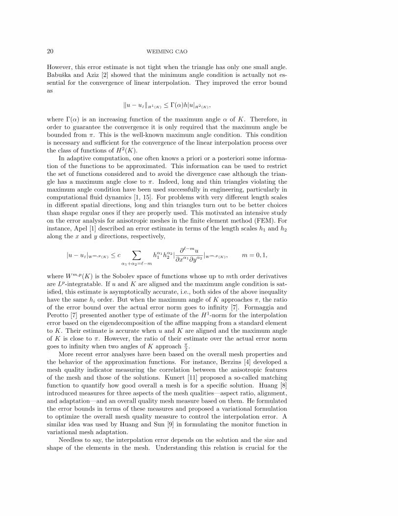
2. Mapping and the geometric characters of a triangle. Let K be a tri-angle in the xy-plane, and let x1,x2, and x3 be the vertices of K. Denote by �ithe vector of the side opposite to xi (in counterclockwise direction). Let K be theequilateral triangle with the vertices

ξ1 =

[01

], ξ2 =

[−

√3

2− 1

2

], ξ3 =

[ √3

2− 1

2

].

The three sides of K are ei =√

3[cos(2(i− 1)π/3), sin(2(i− 1)π/3)]T , i = 1, 2, 3. SeeFigure 1.

ξ1

η

ξ2

ξ3

ξ1

x

y

x2

x3

x1

Fig. 1. Standard element K and physical element K.

Let xc = 13 (x1 + x2 + x3) be the center of K. The affine mapping (which maps

ξi to xi) from K to K can be expressed as x = Mξ + xc with

M =

(1√3(x1 − x3),x2 − xc

).

Denote by M = UΣV ∗ the SVD of the 2 × 2 matrix M . Without loss of generality,we assume Σ = diag(σ1, σ2) with σ1 ≥ σ2 > 0, and

U = Rφu =

[cosφu − sinφu

sinφu cosφu

], V = Rφv =

[cosφv − sinφv

sinφv cosφv

].

Rφu and Rφv represent the linear transform of rotation (counterclockwise) by anglesφu and φv, respectively.

The mapping x = Mξ maps K into a triangle centered at the origin. Its effectcan be understood as the composition of three operations (see, e.g., [16]): (1) rotationclockwise by angle φv; then (2) stretching by factors σ1 and σ2 in ξ and η directions,


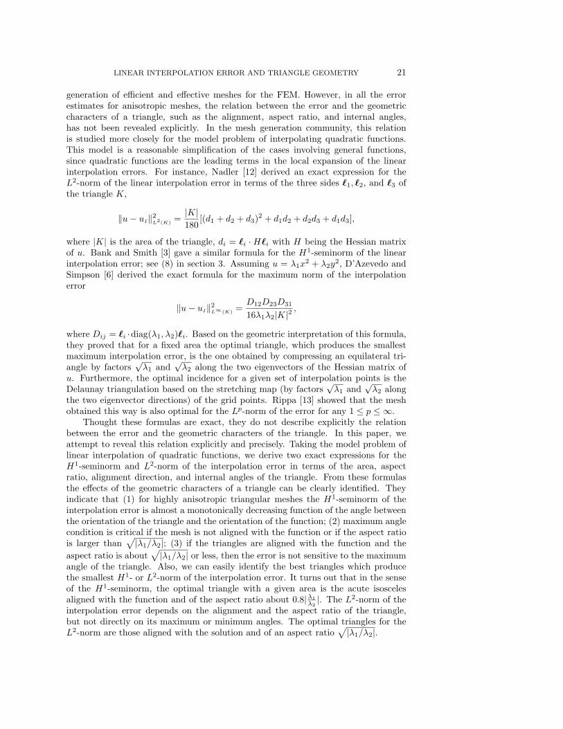
respectively; and finally (3) rotation counterclockwise by angle φu. A circle (centeredat (0,0)) in the ξη-plane will be mapped into an ellipse in the xy-plane with two axesσ1 and σ2, and the longer axis forms an angle φu with the x-axis. See Figure 2.

1 σ1

σ2

ξ1

φv

ξ1

ξ1

φu

Fig. 2. From K to K under the mapping M : R∗φv

K, ΣR∗φv

K, RφuΣR∗φv

K.

We define the aspect ratio of the triangle K as

r12 =σ1

σ2(1)

and define the orientation of K as the direction of angle φu with the x-axis.It can be seen that K is equilateral if and only if σ1 = σ2 and that K is isosceles

if and only if φv = mπ6 with integer m or σ1 = σ2. Together with the aspect ratio,

φv determines the three internal angles of the triangle. For a fixed aspect ratio, themaximum internal angle of K is a periodic even function of φv with period π

3 , andit is decreasing in (0, π

6 ). K is an obtuse isosceles triangle when φv = mπ3 and an

acute isosceles triangle when φv = (2m+1)π6 . If K is an obtuse/acute isosceles, then

its orientation is in parallel/perpendicular to its base. Furthermore, let b and h bethe length of the base and the height over the base of an isosceles triangle; then{

σ1 =√

33 b, σ2 = 2

3h, r12 =√

32

bh , φv = 0 when h ≤

√3

2 b,

σ1 = 23h, σ2 =

√3

3 b, r12 = 2√3hb , φv = π

6 when h >√

32 b.

For general triangles, the aspect ratio r12 can be found as follows. Let

q(K) =1

2

(σ1

σ2+

σ2

σ1

)∈ [1,∞).

This quantity can be calculated from the three sides and the area of K as (see formula(10) below)

q(K) =σ2

1 + σ22

2σ1σ2=

|�1|2 + |�2|2 + |�3|2

4√

3|K|.(2)

Therefore,

r12 = q +√q2 − 1.

Clearly, the closer r12 is to 1, the closer K is to being equilateral. The same istrue for the quantity q(K). Therefore, both r12 and q(K) can be used to measurethe closeness of a triangle to being equilateral. Indeed, the reciprocal of the right-hand-side expression in (2) was used by Bank and Smith [3] as the “shape regularity

24 WEIMING CAO

quantity” of a triangle. q(K) can also be expressed in terms of the matrix M directly.Note that σ1 and σ2 are eigenvalues of (MTM)1/2; it is easy to see that

q(K) =‖M‖2

F

2 det(M),

where ‖ · ‖F stands for the Frobenius norm of a matrix. This formula was used byKnupp, Margolin, and Shashkov [10] in certain functionals characterizing the smooth-ness of the mesh.

There are several other ways to define the aspect ratio and the orientation of atriangular element in the finite element analysis. For instance, the aspect ratio isusually defined as the ratio of the length of the longest side over the perpendiculardistance from it to the opposite vertex, or as the ratio of the diameter of the triangleover the diameter of the largest inscribed circle in the triangle. The orientation canbe defined as the direction of the longest side. It is easy to see that these definitionsare equivalent to (1) up to some bounded constants. However, they are not preciseenough for describing accurately the behavior of the interpolation errors.

3. Formulas for H1- and L2- norms of the interpolation error. Withoutloss of generality, assume K is a triangle with its center at the origin and its orientationbeing the x-axis, i.e., xc = 0, φu = 0. We study the H1- and L2-norms of the error forthe linear interpolation of a quadratic function u over K. Since the first order termsof u have no contribution to the error of linear interpolation, we assume in particularthat u = 1

2x ·Hx, where H is the Hessian of u. Since H is a 2× 2 symmetric matrix,we may decompose it into

H = Rφh

[λ1

λ2

]RT

φh,(3)

where Rφhis the matrix of rotation by an angle φh. We also assume that λ1 ≥ |λ2|.

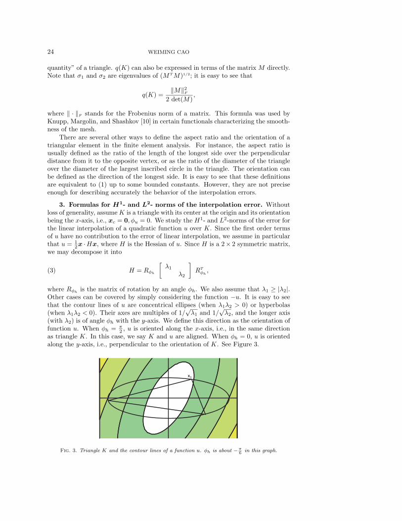
Other cases can be covered by simply considering the function −u. It is easy to seethat the contour lines of u are concentrical ellipses (when λ1λ2 > 0) or hyperbolas(when λ1λ2 < 0). Their axes are multiples of 1/

√λ1 and 1/

√λ2, and the longer axis

(with λ2) is of angle φh with the y-axis. We define this direction as the orientation offunction u. When φh = π

2 , u is oriented along the x-axis, i.e., in the same directionas triangle K. In this case, we say K and u are aligned. When φh = 0, u is orientedalong the y-axis, i.e., perpendicular to the orientation of K. See Figure 3.

x1

Fig. 3. Triangle K and the contour lines of a function u. φh is about −π6

in this graph.


Denote by uI the linear interpolation of u at the three vertices of K. Clearly thenorm of the error u− uI depends on the size and the shape of triangle K, as well asthe magnitude and the orientation of function u. We derive in this section the exactformulas for the H1- and L2-norms of the interpolation error in terms of these factors.

Theorem 3.1. Let K be a triangle oriented along the x-axis. r12 is the aspectratio of K, r21 = 1/r12. Let u be a quadratic function. λ1 and λ2 are the eigenvaluesof the Hessian matrix of u, and the orientation of u is of angle φh with the y-axis;then

‖∇(u− uI)‖2L2(K)

=

√3

36|K|2{

[(r12 + r21)(λ21 + λ2

2) + (r12 − r21)(λ21 − λ2

2) cos(2φh)]

+1

2

[− 4λ1λ2 +

1

4( (λ1 + λ2)(r12 + r21) + (λ1 − λ2)(r12 − r21)(4)

· cos(2φh) )2][(r12 + r21 + (r12 − r21) cos(6φv + 4θ)]

},

where φv is the rotation angle in the mapping from K to K, and

θ =1

2atan

(2(λ1 − λ2) sin(2φh)

(λ1 + λ2)(r12 − r21) + (λ1 − λ2)(r12 + r21) cos(2φh)

).(5)

Proof.

Step 1. We start with a result established by Bank and Smith in [3]. Letci(x, y), i = 1, 2, 3, be the barycentrical coordinates of a point (x, y) in K. The sidebasis functions (taking value 1

4 at a midpoint) are

b1(x, y) = c2(x, y) c3(x, y),b2(x, y) = c3(x, y) c1(x, y),b3(x, y) = c1(x, y) c2(x, y).

It is easy to see that

u− uI = −1

2(v1 b1(x, y) + v2 b2(x, y) + v3 b3(x, y)),(6)

where

vi = �i ·H�i, i = 1, 2, 3.(7)

Let v = [v1, v2, v3]T . It is further established in [3] that∫

K

|∇(u− uI)|2 dxdy =1

4v ·Bv,(8)

where

B =

(∫K

∇bi · ∇bjdxdy

)

= 148|K|

⎡⎣ |�1|2 + |�2|2 + |�3|2 2�1 · �2 2�1 · �3

|�1|2 + |�2|2 + |�3|2 2�2 · �3

symm. |�1|2 + |�2|2 + |�3|2

⎤⎦ .

26 WEIMING CAO

We first derive a formula for the matrix B in terms of the singular values and therotation angle φv of the mapping M . Note that we assume φu = 0; therefore

�i = Mei = ΣR∗φv

ei =√

3

[σ1 cosαi

σ2 sinαi

],

where

αi = 2(i− 1)π/3 − φv, i = 1, 2, 3.(9)

With formula (A.1) in the appendix it is easy to verify that

|�1|2 + |�2|2 + |�3|2 = 3σ21

3∑i=1

cos2 αi + 3σ22

3∑i=1

sin2 αi =9

2(σ2

1 + σ22).(10)

Let

fij =σ2

1

σ21 + σ2

2

cosαi cosαj +σ2

2

σ21 + σ2

2

sinαi sinαj .(11)

Then

�i · �j = 3(σ21 cosαi cosαj + σ2

2 sinαi sinαj) = 3(σ21 + σ2

2)fij , 1 ≤ i, j ≤ 3.

Note that |K| = 3√

34 σ1σ2. We may express B as

B =

√3

24

σ21 + σ2

2

σ1σ2

⎡⎣ 1 4

3f1243f13

1 43f23

symm. 1

⎤⎦ ,

and rewrite the norm of the error as

‖∇(u− uI)‖2L2(K) =

√3

96

σ21 + σ2

2

σ1σ2(12)

·[

3∑i=1

(vi)2 +

8

3(f12 v1v2 + f13 v1v3 + f23 v2v3)

].

Step 2. We next simplify the terms involving vi. Assume the Hessian matrixH = (hij), and denote by

H =

[ σ1

σ2h11 h12

h12σ2

σ1h22

].(13)

Since H is a 2 × 2 symmetric matrix, we may decompose it into

H = Rθ

[μ1

μ2

]RT

θ ,(14)

where Rθ is the matrix for the counterclockwise rotation by an angle θ, and μ1 andμ2 are the eigenvalues of H. By the facts that

vi = �i ·H�i = (R∗φv

ei) · (ΣTHΣ) (R∗φv

ei) = σ1σ2(R∗φv

ei) · H (R∗φv

ei)

= σ1σ2(R∗θR

∗φv

ei) · diag(μ1, μ2) (R∗θR

∗φv

ei)


and that

R∗θR

∗φv

ei =√

3[cos(αi − θ), sin(αi − θ)]T ,

we have

vi = 3σ1σ2[μ1 cos2(αi − θ) + μ2 sin2(αi − θ)]= 3

2σ1σ2[(μ1 + μ2) + (μ1 − μ2) cos 2(αi − θ)].

Therefore it follows from formulas (A.2) and (A.3) that

3∑i=1

(vi)2=

9

4(σ1σ2)

2

[3(μ1 + μ2)

2 +3

2(μ1 − μ2)

2

]

=81

8(σ1σ2)

2

[μ2

1 + μ22 +

2

3μ1μ2

].(15)

Expand vivj as follows:

vivj =9

4(σ1σ2)

2[(μ1 + μ2)2 + (μ2

1 − μ22)(cos 2(αi − θ) + cos 2(αj − θ))(16)

+ (μ1 − μ2)2 cos 2(αi − θ) cos 2(αj − θ)].

Let β = φv + θ. Then αi − θ = 2(i− 1)π/3 − β, and

cos 2(αi − θ) + cos 2(αj − θ) =

⎧⎨⎩

cos(2β + π3 ) for (i, j) = (1, 2),

cos(2β − π3 ) for (i, j) = (1, 3),

cos(2β + π) for (i, j) = (2, 3)

and

cos 2(αi − θ) · cos 2(αj − θ) =

⎧⎪⎨⎪⎩

− 14 − 1

2 cos(4β − π3 ) for (i, j) = (1, 2),

− 14 − 1

2 cos(4β + π3 ) for (i, j) = (1, 3),

− 14 − 1

2 cos(4β + π) for (i, j) = (2, 3).

Substituting the above formulas into (17), we have

f12 v1v2 + f13 v1v3 + f23 v2v3

= 94 (σ1σ2)

2 {[(μ1 + μ2)2 − 1

4 (μ1 − μ2)2] (f12 + f13 + f23)

+ (μ21 − μ2

2) [f12 cos(2β + π3 ) + f13 cos(2β − π

3 ) + f23 cos(2β + π)]

− 12 (μ1 − μ2)

2 [f12 cos(4β − π3 ) + f13 cos(4β + π

3 ) + f23 cos(4β + π)] }.

(17)

By using the definition (11) for fij , we have from formula (A.4) that

f12 + f13 + f23 = −3

4;(18)

from formulas (A.5) and (A.6) that

f12 cos(2β + π3 ) + f13 cos(2β − π

3 ) + f23 cos(2β + π)

= − 34

σ21 − σ2

2

σ21 + σ2

2

cos(2θ);(19)

28 WEIMING CAO

and from formulas (A.7) and (A.8) that

f12 cos(4β − π3 ) + f13 cos(4β + π

3 ) + f23 cos(4β + π)

= − 34

σ21 − σ2

2

σ21 + σ2

2

cos(6φv + 4θ).(20)

Put (17)–(20) into (13); we may express the norm of the error as

‖∇(u− uI)|2L2(K) =3√

3

64(σ2

1 + σ22)σ1σ2

{[μ2

1 + μ22 −

σ21 − σ2

2

σ21 + σ2

2

(μ21 − μ2

2) cos(2θ)

]

+1

2(μ1 − μ2)

2

[1 +

σ21 − σ2

2

σ21 + σ2

2

cos(6φv + 4θ)

]}.(21)

Step 3. Finally we express μ1, μ2, and θ in terms of the eigenvalues of the HessianH and the aspect ratio r12 of K. According to the eigendecomposition (3) of H,

H =

[λ1 cos2 φh + λ2 sin2 φh (λ1 − λ2) sinφh cosφh

(λ1 − λ2) sinφh cosφh λ1 sin2 φh + λ2 cos2 φh

].

Therefore

H = (hij) =

[r12(A + D cos 2φh) D sin 2φh

D sin 2φh r21(A−D cos 2φh)

]

with

A =1

2(λ1 + λ2), D =

1

2(λ1 − λ2).

Recall the eigendecomposition (14), it is not difficult to establish for the eigenvaluesμ1 and μ2 of H that

μ21 + μ2

2 = (h11)2 + (h22)

2 + 2(h12)2

= (A2 + D2 cos2(2φh))(r212 + r2

21) + 2AD(r212 − r2

21) cos(2φh)+ 2D2 sin2(2φh),

(μ21 − μ2

2) cos 2θ = (h11)2 − (h22)

2

= (A2 + D2 cos2(2φh))(r212 − r2

21) + 2AD(r212 + r2

21) cos(2φh),

(μ1 − μ2)2 = (h11 − h22)

2 + 4(h12)2

= 4D2 + A2(r12 − r21)2 + 2AD(r2

12 − r221) cos(2φh)

+D2(r12 − r21)2 cos2(2φh)

= 4(D2 −A2) + A2(r12 + r21)2 + 2AD(r2

12 − r221) cos(2φh)

+D2(r12 − r21)2 cos2(2φh)

= − 4λ1λ2 + [A(r12 + r21) + D(r12 − r21) cos(2φh)]2

and that

tan(2θ) =2h12

h11 − h22

=2D sin 2φh

A(r12 − r21) + D(r12 + r21) cos 2φh.

Substitute the above formulas into the right-hand side of (21) and simplify, and weobtain the formula (5).


We next derive the formula for the L2-norm of the linear interpolation error.Theorem 3.2. Let K be a triangle oriented along the x-axis. r12 is the aspect

ratio of K, r21 = 1/r12. Let u be a quadratic function. λ1 and λ2 are the eigenvaluesof its Hessian, and the orientation of u is of angle φh with the y-axis. Then

‖u− uI‖2L2(K)

=|K|3160

{− 16

9λ1λ2 + [(λ1 + λ2)(r12 + r21)(22)

+ (λ1 − λ2)(r12 − r21) cos(2φh)]2

}.

Proof. It follows from (6) that∫K

|u− uI |2 dxdy =1

4v ·B0v,(23)

where

B0 =

(∫K

bi · bjdxdy).

An elementary calculation of the integrals leads to

B0 =|K|180

⎡⎣ 2 1 1

1 2 11 1 2

⎤⎦ .

Therefore ∫K

|u− uI |2 dxdy =|K|360

(3∑

i=1

(vi)2 + v1v2 + v1v3 + v2v3

),(24)

where v1, v2, and v3 are defined as in (7). We have similar to (17) that

v1v2 + v1v3 + v2v3 =81

16(σ1σ2)

2

(μ2

1 + μ22 +

10

3μ1μ2

),

which, together with (15), yields∫K

|u− uI |2 dxdy =|K|340

((μ1 + μ2)

2 − 4

9μ1μ2

).(25)

Finally, by μ1μ2 = det(H) = det(H) = λ1λ2 and

μ1 + μ2 = h11 + h22 = A(r12 + r21) + D(r12 − r21) cos(2φh),

we prove the conclusion of this theorem.

4. Discussion about some special cases. Denote by T1, T2, and T3 the termsin the square brackets on the right-hand side of (5), i.e.,

T1 = (r12 + r21)(λ21 + λ2

2) + (r12 − r21)(λ21 − λ2

2) cos(2φh),(26)

T2 = −4λ1λ2 +1

4((λ1 + λ2)(r12 + r21) + (λ1 − λ2)(r12 − r21) cos(2φh))

2,(27)

T3 = r12 + r21 + (r12 − r21) cos(6φv + 4θ).(28)

30 WEIMING CAO

Recall that we assume r12 = σ1/σ2 ≥ 1 and λ1 ≥ |λ2|; therefore all the three termsabove are nonnegative, and we may write

‖∇(u− uI)‖2L2(K)

=

√3

36|K|2(T1 +

1

2T2 · T3

).(29)

We may also restrict 0 ≤ φv < π3 and 0 ≤ φh < π. Other cases are covered by the

symmetry and periodicity of the error norms. For a fixed aspect ratio, the extremumvalues of T1, T2, and T3 are

T1=

{min (T1) = 2(r21λ

21 + r12λ

22) when φh = π

2 ,max (T1) = 2(r12λ

21 + r21λ

22) when φh = 0,

(30)

T2=

{min (T2) = (r21λ1 − r12λ2)

2 when φh = π2 ,

max (T2) = (r12λ1 − r21λ2)2 when φh = 0,

(31)

T3=

{min (T3) = 2r21 when 6φv + 4θ = (2m + 1)π,max (T3) = 2r12 when 6φv + 4θ = 2mπ.

(32)

We give more details about these cases.Case 1. φh = π

2 and φv = π6 , i.e., K is an acute isosceles triangle aligned with u.

In this case, θ = 0 by (5). Therefore, T1, T2, and T3 all take their minimum values,which yields

‖∇(u− uI)‖2L2(K)

=

√3

36|K|2 [ 2(r21λ

21 + r12λ

22) + r21(r21λ1 − r12λ2)

2 ].(33)

This is the smallest H1-seminorm of the interpolation error for all the triangles witha fixed aspect ratio and a fixed area.

We may consider the optimal choice of the aspect ratio in this case. Let

f(r) = 2(

1r λ

21 + rλ2

2

)+ 1

r

(1r λ1 − rλ2

)2= 3λ2

2r + 2(2λ21 − 4λ1λ2)

1r + λ2

11r3 .

It can be seen that f is decreasing in [1, r(1)∗ ) and increasing in (r

(1)∗ ,∞), where

r(1)∗ =

√√√√λ1(λ1 − λ2) + λ1

√(λ1 − λ2)2 + 9λ2

2

3λ22

.(34)

Therefore r12 = r(1)∗ is the best aspect ratio. Moreover, since T1, T2, and T3 all take

minimum values in this case, we conclude that the acute isosceles triangle, which is

aligned with u and of the aspect ratio r(1)∗ , is the best one that produces the smallest

H1-seminorm of the interpolation error among all the triangles with the same area!

It is noted that for u with λ1 = λ2 (isotropic u), the best aspect ratio is r(1)∗ = 1

(with isotropic K). For u with λ2 = −λ1, the best aspect ratio is r(1)∗ =

√(2 +

√13)/3

≈ 1.367. When λ1 >> |λ2|, we have

r(1)∗ ≈

√2

3

∣∣∣∣λ1

λ2

∣∣∣∣ ≈ 0.816

∣∣∣∣λ1

λ2

∣∣∣∣ ,


with which the interpolation error is of the smallest possible magnitude

‖∇(u− uI)‖2L2(K)

≈√

2

6|K|2|λ1λ2| ≈ 0.235|K|2|λ1λ2|.(35)

We may also compare the above optimal choice of the aspect ratio with someintuitive choices. For instance, if we choose r12 = 1, then

‖∇(u− uI)‖2L2(K)

≈√

3

36|K|2(3(λ2

1 + λ22) − 2λ1λ2),(36)

which is between 0.128|K|2λ21 and 0.193|K|2λ2

1. If we choose r12 = |λ1λ2

|, then in the

case λ1 >> |λ2|,

‖∇(u− uI)‖2L2(K)

≈ 5√

3

36|K|2|λ1λ2| ≈ 0.240|K|2|λ1λ2|;(37)

if we choose r12 =√|λ1/λ2|, then we have

‖∇(u− uI)‖2L2(K)

=

√3

18|K|2√|λ3

1λ2| ≈ 0.0962|K|2√|λ3

1λ2|.(38)

Note that when u and K are aligned, the inverse mapping ξ = M−1x with r12 =√|λ1/λ2| transforms u(x, y) into const.(ξ2 ± η2) and K into an equilateral triangle.

It was shown by D’Azevedo and Simpson [6] and Rippa [13] that triangles with suchan aspect ratio lead to the smallest maximum-norm and Lp-norm of the interpolationerror among all triangles of the same area. However, this aspect ratio is not theoptimal for the interpolation error in the sense of H1-seminorm.

Case 2. φh = π2 and φv = 0, i.e., K is an obtuse isosceles triangle aligned with u.

We have in this case

‖∇(u− uI)‖2L2(K)

=

√3

36|K|2 [ 2(r21λ

21 + r12λ

22) + r12(r21λ1 − r12λ2)

2 ].(39)

This error formula differs from that of Case 1 only in the coefficient of the secondterm.

To study the optimal choice of the aspect ratio in this case, let

g(r) = 2(

1r λ

21 + rλ2

2

)+ r(

1r λ1 − rλ2

)2= 3λ2

11r + 2(λ2

2 − λ1λ2)r + λ22r

3.

It can be shown that the minimum of g is attained at

r(2)∗ =

√√√√λ2(λ1 − λ2) + |λ2|√

(λ1 − λ2)2 + 9λ22

3λ22

.(40)

When λ1 = λ2, the best aspect ratio is r(2)∗ = 1. When λ2 = −λ2, the best aspect

ratio is r(1)∗ =

√(2 +

√13)/3 ≈ 1.367. When |λ1| >> |λ2|, we have

r(2)∗ ≈

⎧⎪⎪⎨⎪⎪⎩

√√10 + 1

3 |λ1λ2

| ≈ 1.178

√|λ1λ2

| when λ1λ2 > 0,√√10 − 1

3 |λ1λ2

| ≈ 0.849

√|λ1λ2

| when λ1λ2 < 0.

32 WEIMING CAO

With this choice of aspect ratio, the interpolation error is of the magnitude

‖∇(u− uI)‖2L2(K)

≈{

0.0878|K|2√|λ3

1λ2| when λ1λ2 > 0,

0.281|K|2√|λ3

1λ2| when λ1λ2 < 0.(41)

We may compare this case (obtuse isosceles) with the previous one (acute isosce-les). When the triangle is aligned with u and the aspect ratio r12 ≈

√|λ1/λ2|, the

interpolation error is nearly the same for both acute and obtuse triangles if λ1λ2 > 0.For u with λ1λ2 < 0, ‖∇(u − uI)‖L2(K) is about 1.7 times smaller with the acuteisosceles triangle than that with the obtuse one. Furthermore, because for generaltriangles with arbitrary φv, the error norm ‖∇(u−uI)‖L2(K) is between those of Case1 and Case 2, we may conclude that the H1-seminorm of the interpolation error isnot sensitive to the maximum angle of the triangle, as long as the triangle is alignedwith the function u and the aspect ratio r12 ≈

√|λ1/λ2| is used.

Case 3. φh = 0. In this case the orientation of u is perpendicular to the triangle.We have

‖∇(u− uI)‖2L2(K)

=

√3

18|K|2 [2(r12λ

21 + r21λ

22) + (r12λ1 − r21λ2)

2

· (r12 + r21 + (r12 − r21) cos(6φv))](42)

For given |K| and φv, it can be shown the error norm is an increasing function of r12.Therefore, the best aspect ratio is r12 = 1. This is not surprising, since when thetriangle is perpendicular to the orientation of u, increasing the aspect ratio leads tolower resolution in the needy direction and larger interpolation error, no matter whatvalue φv takes.

We should emphasize that in the above discussion on the optimal aspect ratiosthe area and the orientation of the triangle are assumed fixed. In adaptive meshgeneration there may be some other constraints on the triangles in a mesh, e.g., oneside of a triangle or the vertices of the triangles are fixed. Optimal choices of theaspect ratio subject to those constraints can be quite different from the above values.

5. General discussion about orientation, aspect ratio, and angle con-dition. In this section we present a general discussion about the effects of the ori-entation, aspect ratio, and the angle φv. We first study the H1-seminorm of theinterpolation error.

Mesh alignment. Given a triangle K (fixed |K|, r12, and φv), it is commonlybelieved that the interpolation error is the smallest when the triangle is aligned withthe function, i.e., when φh = π

2 . We present a justification of this viewpoint. Weconsider the case where both the solutions and the triangles are highly anisotropic,i.e., we assume λ1 >> |λ2| and r12 >> 1. In this case we have for the three terms(26)–(28) in the error norm ‖∇(u− uI)‖2

L2(K)that

T1 = r12λ21(1 + cos 2φh) + LOT,

T2 = 14 (r12λ1)

2(1 + cos 2φh)2 + LOT,T3 = r12(1 + cos(6φv + 4θ)) + LOT

and for the angle θ in (5) that

tan(2θ) ≈ 2λ1 sin 2φh

λ1r12(1 + cos 2φh)= 2r21 tanφh,


where the lower order terms LOT include r12λ22, r12λ

21, r21λ

22, etc. In this case the

error norm is dominated by

‖∇(u− uI)‖2L2(K)

≈√

336 |K|2 [r12λ

21 + 1

4r312λ

21(1 + cos 2φh)(1 + cos(6φv + 4θ))]

· (1 + cos 2φh) + LOT.

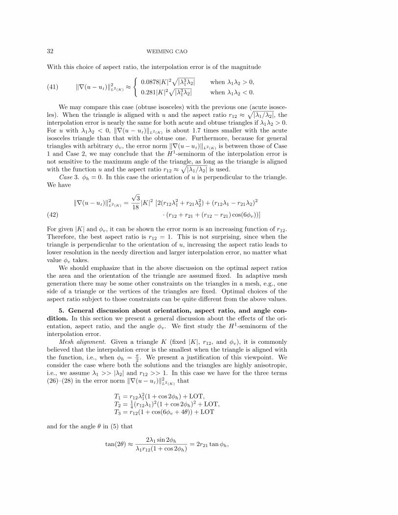
Note that by (5) θ is an increasing function of φh, and cos(2φh) is a decreasingfunction of φh in (0, π

2 ). Therefore, we may conclude that the H1-seminorm of theerror is almost a monotonically decreasing function of the angle φh in (0, π

2 ).We plot in Figure 4 the graph of ‖∇(u − uI)‖2

L2(K)versus φh for various λ1, λ2,

φv and r12. It is observed that for all aspect ratios and φv, the error is smallest whenφh is near π

2 . Also seen in Figure 4 is a small peak of the error norm around φh = π2 .

This is because when φh is very close to π2 , the leading terms in T1 and T2 go to 0

and the lower order terms become the major components in the error.

0 0.2 0.4 0.6 0.8 110

0

101

102

103

104

with λ1=10, λ

2=1, r

12=8

||∇(u

-uL)|

|2 (K)

φv=0

φv=π/8

φv=π/6

0 0.2 0.4 0.6 0.8 110

0

101

102

103

with λ1=10, λ

2=1, r

12=4

||∇(u

-uL)|

|2 (K)

φv=0

φv=π/8

φv=π/6

0 0.2 0.4 0.6 0.8 110

0

105

1010

with λ1=100, λ

2=1, r

12=80

||∇(u

-uL)|

|2 (K)

φv=0

φv=π/8

φv=π/6

0 0.2 0.4 0.6 0.8 110

0

102

104

106

108

with λ1=100, λ

2=1, r

12=40

||∇(u

-u L)|

|2 (K)

φv=0

φv=π/8

φv=π/6

Fig. 4. ‖u− uI‖2L2(K)

versus the alignment angle φh/π with |K| = 3√

34

fixed.

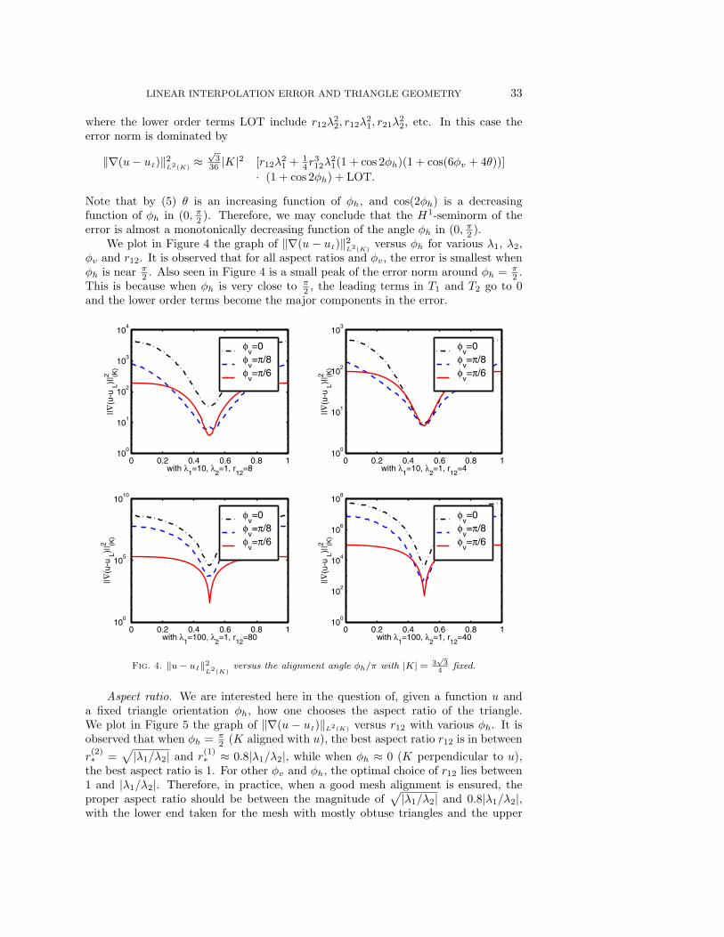
Aspect ratio. We are interested here in the question of, given a function u anda fixed triangle orientation φh, how one chooses the aspect ratio of the triangle.We plot in Figure 5 the graph of ‖∇(u − uI)‖L2(K) versus r12 with various φh. It isobserved that when φh = π

2 (K aligned with u), the best aspect ratio r12 is in between

r(2)∗ =

√|λ1/λ2| and r

(1)∗ ≈ 0.8|λ1/λ2|, while when φh ≈ 0 (K perpendicular to u),

the best aspect ratio is 1. For other φv and φh, the optimal choice of r12 lies between1 and |λ1/λ2|. Therefore, in practice, when a good mesh alignment is ensured, theproper aspect ratio should be between the magnitude of

√|λ1/λ2| and 0.8|λ1/λ2|,

with the lower end taken for the mesh with mostly obtuse triangles and the upper

34 WEIMING CAO

0 10 20 30 4010

0

101

102

103

104

with φh=π/2

||∇(u

-uL)|

|2 (K)

φv=0

φv=π/8

φv=π/6

0 10 20 30 4010

1

102

103

104

105

with φh=π/3

||∇(u

-u L)|

|2 (K)

φv=0

φv=π/8

φv=π/6

0 10 20 30 4010

0

102

104

106

with φh=π/6

||∇(u

-u L)|

|2 (K)

φv=0

φv=π/8

φv=π/6

0 10 20 30 4010

0

102

104

106

with φh=0

||∇(u

-u L)|

|2 (K)

φv=0

φv=π/8

φv=π/6

Fig. 5. ‖∇(u− uI)‖2L2(K)

versus the aspect ratio r12 with λ1 = 10, λ2 = 1, and |K| = 3√

34

.

end taken for the mesh with mostly acute triangles. The less the mesh alignment, thesmaller r12 should be.

Maximum angle condition. It is well known that a good mesh for finite el-ement approximation should respect the so-called maximum angle condition, i.e.,the maximum angles of the triangular elements should be bounded from π. In [2],Babuska and Aziz gave an example showing that when the maximum angle con-dition is violated, the H1-seminorm of the error of linear interpolation can go toinfinity, although the element area approaches 0. Their example is in our nota-

tion the case with λ1 = 1, λ2 = 0, |K| = ε2 , r12 =

√3

2ε , φh = 0, φv = 0, and thus‖∇(u − uI)‖2

L2(K)= 9

256 (ε + 38ε ). We discuss here the impact of the maximum angle

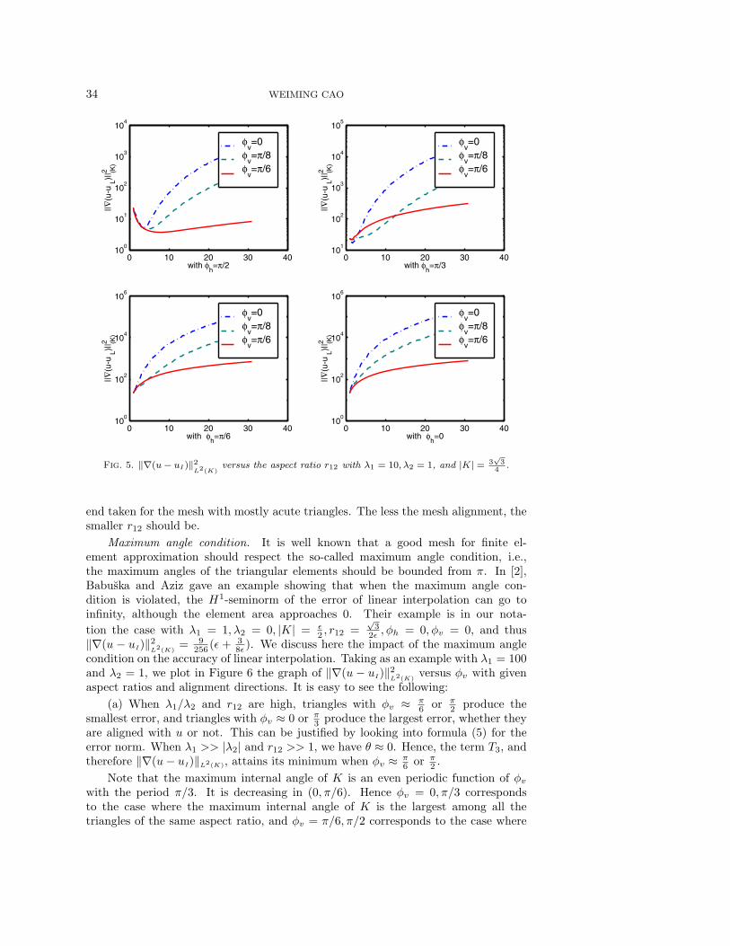
condition on the accuracy of linear interpolation. Taking as an example with λ1 = 100and λ2 = 1, we plot in Figure 6 the graph of ‖∇(u − uI)‖2

L2(K)versus φv with given

aspect ratios and alignment directions. It is easy to see the following:

(a) When λ1/λ2 and r12 are high, triangles with φv ≈ π6 or π

2 produce thesmallest error, and triangles with φv ≈ 0 or π

3 produce the largest error, whether theyare aligned with u or not. This can be justified by looking into formula (5) for theerror norm. When λ1 >> |λ2| and r12 >> 1, we have θ ≈ 0. Hence, the term T3, andtherefore ‖∇(u− uI)‖L2(K), attains its minimum when φv ≈ π

6 or π2 .

Note that the maximum internal angle of K is an even periodic function of φv

with the period π/3. It is decreasing in (0, π/6). Hence φv = 0, π/3 correspondsto the case where the maximum internal angle of K is the largest among all thetriangles of the same aspect ratio, and φv = π/6, π/2 corresponds to the case where


the maximum internal angle is the smallest among all triangles. Therefore, in thiscase it is important to use triangles with smaller maximum internal angles, regardlessof whether or not the mesh alignment is satisfied.

(b) When the triangle is aligned with u and the aspect ratio r12 ≈√|λ1/λ2|, the

error is insensitive to φv and is therefore insensitive to the maximum internal angleof the triangle. In particular, if φh = π

2 , λ1λ2 > 0, and r12 =√

λ1/λ2, then T2 = 0,and by (29) ‖∇(u−uI)‖L2(K) is independent of φv. See the lower left graph of Figure6 and the analysis in Cases 1 and 2 in section 4.

(c) When r12 ≈ 1, the best φv may be different from π6 and π

2 . However, inthis case the difference between the maximum and the minimum of the error is notsignificant.

0 0.2 0.4 0.6 0.8 110

0

105

1010

with λ1=100, λ

2=1, r

12=80

||∇(u

-uL)|

|2 (K)

φh=0

φh=π/6

φh=π/3

φh=π/2

0 0.2 0.4 0.6 0.8 110

0

102

104

106

108

with λ1=100, λ

2=1, r

12=20

||∇(u

-u L)|

|2 (K)

φh=0

φh=π/6

φh=π/3

φh=π/2

0 0.2 0.4 0.6 0.8 110

2

103

104

105

106

with λ1=100, λ

2=1, r

12=10

||∇(u

-u L)|

|2 (K)

φh=0

φh=π/6

φh=π/3

φh=π/2

0 0.2 0.4 0.6 0.8 110

3

104

with λ1=100, λ

2=1, r

12=1.5

||∇(u

-u L)|

|2 (K)

φh=0

φh=π/6

φh=π/3

φh=π/2

Fig. 6. ‖∇(u− uI)‖2L2(K)

versus the angle φv/π with |K| = 3√

34

fixed.

In summary, we conclude that if the triangle is aligned with the function andthe aspect ratio is of an magnitude

√|λ1/λ2| or smaller, then the maximum angle

condition is not essential to the H1-seminorm of the interpolation error. Otherwise,the maximum angle is critical to the magnitude of the error.

L2-norm. From (23) we can conclude the following for the L2-norm of the linearinterpolation error:

(1) ‖u−uI‖L2(K) does not depend on the angle φv. Therefore, for a given function,the L2-norm of its linear interpolation error depends only on the area, aspect ratio,and orientation of the triangle. Maximum/minimum angle conditions are irrelevantto the L2-norm of the interpolation error.

(2) ‖u − uI‖L2(K) is a π-periodic even function of φh. It is decreasing in φh in

36 WEIMING CAO

(0, π2 ). When φh = π

2 (K aligned with u),

‖u− uI‖2L2(K)

=|K|340

[(λ1r21 + λ2r12)

2 − 4

9λ1λ2

]

is the smallest, and when φh = 0 (K perpendicular to u)

‖u− uI‖2L2(K)

=|K|340

[(λ1r12 + λ2r21)

2 − 4

9λ1λ2

]

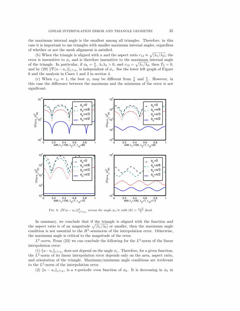
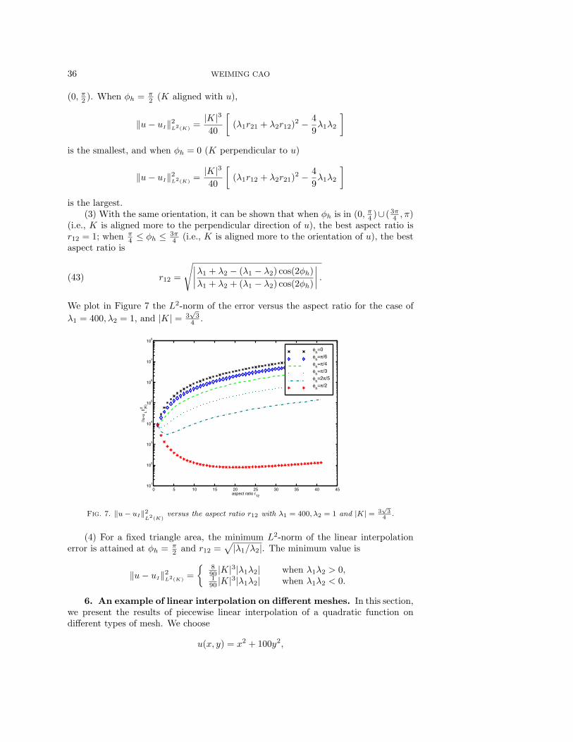
is the largest.(3) With the same orientation, it can be shown that when φh is in (0, π

4 )∪ ( 3π4 , π)

(i.e., K is aligned more to the perpendicular direction of u), the best aspect ratio isr12 = 1; when π

4 ≤ φh ≤ 3π4 (i.e., K is aligned more to the orientation of u), the best

aspect ratio is

r12 =

√∣∣∣∣λ1 + λ2 − (λ1 − λ2) cos(2φh)

λ1 + λ2 + (λ1 − λ2) cos(2φh)

∣∣∣∣ .(43)

We plot in Figure 7 the L2-norm of the error versus the aspect ratio for the case of

λ1 = 400, λ2 = 1, and |K| = 3√

34 .

0 5 10 15 20 25 30 35 40 4510

1

102

103

104

105

106

107

108

aspect ratio r12

||u-u

L||2 (K)

φh=0

φh=π/6

φh=π/4

φh=π/3

φh=2π/5

φh=π/2

Fig. 7. ‖u− uI‖2L2(K)

versus the aspect ratio r12 with λ1 = 400, λ2 = 1 and |K| = 3√

34

.

(4) For a fixed triangle area, the minimum L2-norm of the linear interpolationerror is attained at φh = π

2 and r12 =√|λ1/λ2|. The minimum value is

‖u− uI‖2L2(K)

=

{890 |K|3|λ1λ2| when λ1λ2 > 0,190 |K|3|λ1λ2| when λ1λ2 < 0.

6. An example of linear interpolation on different meshes. In this section,we present the results of piecewise linear interpolation of a quadratic function ondifferent types of mesh. We choose

u(x, y) = x2 + 100y2,


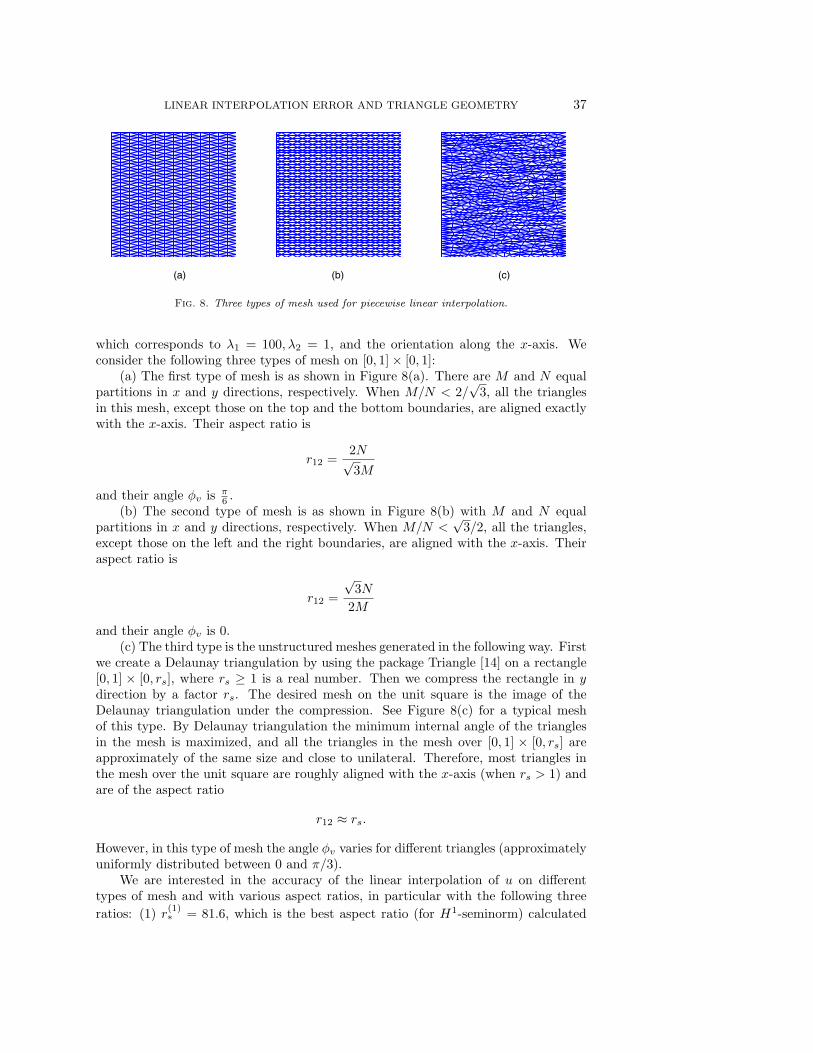
(a) (b) (c)

Fig. 8. Three types of mesh used for piecewise linear interpolation.

which corresponds to λ1 = 100, λ2 = 1, and the orientation along the x-axis. Weconsider the following three types of mesh on [0, 1] × [0, 1]:

(a) The first type of mesh is as shown in Figure 8(a). There are M and N equalpartitions in x and y directions, respectively. When M/N < 2/

√3, all the triangles

in this mesh, except those on the top and the bottom boundaries, are aligned exactlywith the x-axis. Their aspect ratio is

r12 =2N√3M

and their angle φv is π6 .

(b) The second type of mesh is as shown in Figure 8(b) with M and N equalpartitions in x and y directions, respectively. When M/N <

√3/2, all the triangles,

except those on the left and the right boundaries, are aligned with the x-axis. Theiraspect ratio is

r12 =

√3N

2M

and their angle φv is 0.(c) The third type is the unstructured meshes generated in the following way. First

we create a Delaunay triangulation by using the package Triangle [14] on a rectangle[0, 1] × [0, rs], where rs ≥ 1 is a real number. Then we compress the rectangle in ydirection by a factor rs. The desired mesh on the unit square is the image of theDelaunay triangulation under the compression. See Figure 8(c) for a typical meshof this type. By Delaunay triangulation the minimum internal angle of the trianglesin the mesh is maximized, and all the triangles in the mesh over [0, 1] × [0, rs] areapproximately of the same size and close to unilateral. Therefore, most triangles inthe mesh over the unit square are roughly aligned with the x-axis (when rs > 1) andare of the aspect ratio

r12 ≈ rs.

However, in this type of mesh the angle φv varies for different triangles (approximatelyuniformly distributed between 0 and π/3).

We are interested in the accuracy of the linear interpolation of u on differenttypes of mesh and with various aspect ratios, in particular with the following three

ratios: (1) r(1)∗ = 81.6, which is the best aspect ratio (for H1-seminorm) calculated

38 WEIMING CAO

according to (34) for the case of acute isosceles triangles; (2) r(2)∗ = 11.79, which

is the best aspect ratio (in H1-seminorm) calculated according to (40) for the case

of obtuse isosceles triangles; and (3) r(∞)∗ =

√|λ1

λ2| = 10, which is the best aspect

ratio for the Lp-norm, 1 ≤ p ≤ ∞. We also report the results with the aspect ratiosr12 = λ1/λ2 = 10 and r12 = 1.

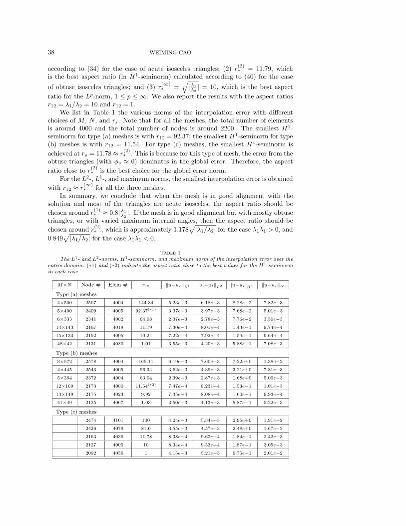
We list in Table 1 the various norms of the interpolation error with differentchoices of M , N , and rs. Note that for all the meshes, the total number of elementsis around 4000 and the total number of nodes is around 2200. The smallest H1-seminorm for type (a) meshes is with r12 = 92.37; the smallest H1-seminorm for type(b) meshes is with r12 = 11.54. For type (c) meshes, the smallest H1-seminorm is

achieved at rs = 11.78 ≈ r(2)∗ . This is because for this type of mesh, the error from the

obtuse triangles (with φv ≈ 0) dominates in the global error. Therefore, the aspect

ratio close to r(2)∗ is the best choice for the global error norm.

For the L2-, L1-, and maximum norms, the smallest interpolation error is obtained

with r12 ≈ r(∞)∗ for all the three meshes.

In summary, we conclude that when the mesh is in good alignment with thesolution and most of the triangles are acute isosceles, the aspect ratio should be

chosen around r(1)∗ ≈ 0.8|λ1

λ2|. If the mesh is in good alignment but with mostly obtuse

triangles, or with varied maximum internal angles, then the aspect ratio should be

chosen around r(2)∗ , which is approximately 1.178

√|λ1/λ2| for the case λ1λ1 > 0, and

0.849√|λ1/λ2| for the case λ1λ1 < 0.

Table 1

The L1- and L2-norms, H1-seminorm, and maximum norm of the interpolation error over theentire domain. (∗1) and (∗2) indicate the aspect ratio close to the best values for the H1 seminormin each case.

M×N Node # Elem # r12 ‖u−uI‖L1 ‖u−uI‖L2 |u−uI |H1 ‖u−uI‖∞

Type (a) meshes

4×500 2507 4004 144.34 5.23e−3 6.18e−3 8.28e−2 7.82e−3

5×400 2409 4005 92.37(∗1) 3.37e−3 3.97e−3 7.68e−2 5.01e−3

6×333 2341 4002 64.08 2.37e−3 2.78e−3 7.76e−2 3.50e−3

14×143 2167 4018 11.79 7.30e−4 8.01e−4 1.43e−1 9.74e−4

15×133 2152 4005 10.24 7.22e−4 7.92e−4 1.54e−1 9.64e−4

48×42 2131 4080 1.01 3.55e−3 4.20e−3 5.88e−1 7.08e−3

Type (b) meshes

3×572 2578 4004 165.11 6.19e−3 7.60e−3 7.22e+0 1.38e−2

4×445 2543 4005 96.34 3.62e−3 4.39e−3 3.21e+0 7.81e−3

5×364 2372 4004 63.04 2.39e−3 2.87e−3 1.68e+0 5.00e−3

12×160 2173 4000 11.54(∗2) 7.47e−4 8.23e−4 1.53e−1 1.01e−3

13×149 2175 4023 9.92 7.35e−4 8.08e−4 1.60e−1 9.93e−4

41×49 2125 4067 1.03 3.50e−3 4.13e−3 5.87e−1 5.22e−3

Type (c) meshes

2474 4101 100 4.24e−3 5.34e−3 2.95e+0 1.91e−2

2426 4079 81.6 3.55e−3 4.57e−3 2.48e+0 1.67e−2

2163 4036 11.78 8.38e−4 9.62e−4 1.84e−1 2.42e−3

2127 4005 10 8.34e−4 9.53e−4 1.87e−1 3.05e−3

2092 4036 1 4.15e−3 5.21e−3 6.75e−1 2.01e−2


Appendix. We list here some basic trigonometric formulas used to derive theresults in the previous sections. Let α be any real number. Denote by αi = 2(i −1)π/3 − α, i = 1, 2, 3.

(A.1) cos2(α1) + cos2(α2) + cos2(α3) =3

2,

(A.2) cos(2α1) + cos(2α2) + cos(2α3) = 0,

(A.3) cos2(2α1) + cos2(2α2) + cos2(2α3) =3

2,

(A.4) cos(α1) cos(α2) + cos(α1) cos(α3) + cos(α2) cos(α3) = −3

4.

Similar relations hold for sine functions, too.

Let θ be any real number, and let β = α + θ. Then

(A.5) cos(α1) cos(α2) cos(2β +

π

3

)+ cos(α1) cos(α3) cos

(2β − π

3

)+ cos(α2) cos(α3) cos(2β + π) = −3

4cos(2θ),

(A.6) sin(α1) sin(α2) cos(2β +

π

3

)+ sin(α1) sin(α3) cos

(2β − π

3

)+ sin(α2) sin(α3) cos(2β + π) =

3

4cos(2θ),

(A.7) cos(α1) cos(α2) cos(4β − π

3

)+ cos(α1) cos(α3) cos

(4β +

π

3

)+ cos(α2) cos(α3) cos(4β + π) = −3

4cos(6α + 4θ),

(A.8) sin(α1) sin(α2) cos(4β − π

3

)+ sin(α1) sin(α3) cos

(4β +

π

3

)+ sin(α2) sin(α3) cos(4β + π) =

3

4cos(6α + 4θ).

REFERENCES

[1] T. Apel, Anisotropic Finite Elements: Local Estimates and Applications, Adv. Numer. Math.,Teubner, Stuttgart, 1999.

[2] I. Babuska and A. K. Aziz, On the angle condition in the finite element method, SIAM J.Numer. Anal., 13 (1976), pp. 214–226.

[3] R. E. Bank and R. K. Smith, Mesh smoothing using a posteriori error estimates, SIAM J.Numer. Anal., 34 (1997), pp. 979–997.

[4] M. Berzins, A solution-based triangular and tetrahedral mesh quality indicator, SIAM J. Sci.Comput., 19 (1998), pp. 2051–2060.

[5] J. Bramble and M. Zlamal, Triangular elements in the finite element method, Math. Comp.,24 (1970), pp. 809–820.

[6] E. F. D’Azevedo and R. B. Simpson, On optimal interpolation triangle incidences, SIAM J.Sci. Statist. Comput., 10 (1989), pp. 1063–1075.

[7] L. Formaggia and S. Perotto, New anisotropic a priori error estimates, Numer. Math., 89(2001), pp. 641–667.

[8] W. Huang, Measuring mesh qualities and application to variational mesh adaptation, SIAMJ. Sci. Comput., 26 (2005), pp. 1643–1666.

[9] W. Huang and W. Sun, Variational mesh adaptation II: Error estimates and monitor func-tions, J. Comput. Phys., 184 (2003), pp. 619–648.

[10] P. Knupp, L. G. Margolin, and M. Shashkov, Reference Jacobian optimization-based rezonestrategies for arbitrary Lagrange Eulerian methods, J. Comput. Phys., 176 (2002), pp. 93–128.

40 WEIMING CAO

[11] G. Kunert, A Posteriori Error Estimation for Anisotropic Tetrahedral and Triangular FiniteElement Meshes, Ph.D. dissertation, TU Chemnitz, Chemnitz, Germany, 1999.

[12] E. J. Nadler, Piecewise Linear Approximation on Triangulations of a Planar Region, Ph.D.thesis, Division of Applied Mathematics, Brown University, Providence, RI, 1985.

[13] S. Rippa, Long and thin triangles can be good for linear interpolation, SIAM J. Numer. Anal.,29 (1992), pp. 257–270.

[14] J. R. Shewchuk, Triangle: Engineering a 2D Quality Mesh Generator and Delaunay Trian-gulator, Technical report, School of Computer Science, Carnegie Mellon University, Pitts-burgh, PA, 1996.

[15] R. B. Simpson, Anisotropic mesh transformations and optimal error control, Appl. Numer.Math., 14 (1994), pp. 183–198.

[16] L. N. Trefethen and D. Bau, Numerical Linear Algebra, SIAM, Philadelphia, 1997.

Documents

ON THE ERROR OF LINEAR INTERPOLATION AND THE