On the Exact Analytical and Numerical Solutions of Nano

Hindawi Publishing CorporationAbstract and Applied AnalysisVolume 2012, Article ID 415431, 22 pagesdoi:10.1155/2012/415431

Research ArticleOn the Exact Analytical and Numerical Solutions ofNano Boundary-Layer Fluid Flows

Emad H. Aly1, 2 and Abdelhalim Ebaid3

1 Department of Mathematics, Faculty of Science, King Abdulaziz University, Jeddah 21589, Saudi Arabia2 Department of Mathematics, Faculty of Education, Ain Shams University, Roxy, Cairo 11757, Egypt3 Department of Mathematics, Faculty of Science, Tabuk University, Tabuk 71491, Saudi Arabia

Correspondence should be addressed to Emad H. Aly, [email protected]

Received 31 May 2012; Revised 24 July 2012; Accepted 25 July 2012

Academic Editor: Svatoslav Stanek

Copyright q 2012 E. H. Aly and A. Ebaid. This is an open access article distributed under theCreative Commons Attribution License, which permits unrestricted use, distribution, andreproduction in any medium, provided the original work is properly cited.

The nonlinear boundary value problem describing the nanoboundary-layer flow with linearNavier boundary condition is investigated theoretically and numerically in this paper. The G′/G-expansion method is applied to search for the all possible exact solutions, and its results are thenvalidated by the Chebyshev pseudospectral differentiation matrix (ChPDM) approach which hasbeen recently introduced and successfully used. This numerical technique is firstly applied and, oncomparing with the other recent work, it is found that the results are very accurate and effectiveto deal with the current problem. It is then used to examine and validate the present analyticalanalysis. Although the G′/G-expansion method has been used widely to solve nonlinear waveequations, its application for nonlinear boundary value problems has not been discussed yet, andthe present paper may be the first to address this point. It is clarified that the exact solutionsobtained via the G′/G-expansion method cannot be obtained by using some of the other methods.In addition, the domain of the physical parameters involved in the current boundary valueproblem is also discussed. Furthermore, the convex, vicinity of zero, and asymptotic solutionsare deduced.

1. Introduction

At nanoscale diameters, it was shown in an interesting paper by He et al. [1] that a fascinatingphenomena arise when the diameter of the electrospun nanofibers is less than 100 nm.The nanoeffect has been demonstrated for unusual strength, high surface energy, surfacereactivity, and high thermal and electric conductivity.

The notion of a boundary layer was first introduced by Prandtl [2] over a hundredyears ago to explain the discrepancies between the theory of inviscid fluid flow and exper-iment. In the classical boundary-layer theory, the condition of no-slip near the solid walls

2 Abstract and Applied Analysis

is usually applied, where the fluid velocity component is assumed to be zero relative tothe solid boundary. However, this is not true for fluid flows at the micro- and nanoscale.Investigations show that the no-slip condition is no longer valid, and instead, a certaindegree of tangential slipmust be allowed [3]. In words, nanoboundary-layer fluid flowsmeannanoscale flows which have many applications in microelectromechanical systems. Becauseof the microscale dimensions of these devices, the fluid flow behavior deviates significantlyfrom the traditional no-slip flow. In recent years, some interest has been given to the studyof this type of flow, and some useful results have been introduced by many authors, see, forexample, [4–12].

In this paper we consider themodel proposed byWang [8] to describe the viscous flowdue to a stretching surface with both surface slip and suction (or injection). He consideredtwo geometries situations, namely, the two-dimensional and axisymmetric of a stretchingsurface. Wang [8] applied a similarity transform to convert the Navier-Stokes equations intoa 3rd-order nonlinear ordinary differential equation given by

f ′′′(η)+mf

(η)f ′′(η

) − [f ′(η)

]2 = 0, (1.1)

where m is a parameter describing the type of stretching, where m = 1 describes the two-dimensional stretching, while m = 2 is for axisymmetric stretching. The flow is subjected tothe following boundary conditions:

f(0) = s, f ′(0) = 1 + λf ′′(0), f ′(∞) = 0, (1.2)

where λ > 0 is a nondimensional slip parameter, and s < 0 when injection from the surfaceoccurs and s > 0 for suction.

During the past two decades, much effort has been spent on searching for exactsolutions of nonlinear equations due to their importance in understanding its phenomena.In order to achieve this goal, various direct methods have been proposed, such as tanh-function [13], Jacobi-elliptic function [14], F-expansion [15], exp-function ([16–20]), thegeneralized exp-function [21], G′/G-expansion ([22, 23]), generalized G′/G-expansion [24],and simplified G′/G-expansion [25]. However, a little attention was devoted for theirapplications to solving nonlinear boundary value problems (BVPs). It should be noted thatthe current work may be the first to indicate the way of applying theG′/G-expansion methodto solve BVPs, where the advantages of the current method over some of the other onesmentioned above are clarified later in this paper.

In order to solve the BVP given by (1.1) and (1.2), Van Gorder et al. [11] applied thehomotopy analysis method. They have also discussed the effects of the slip parameter λ andthe suction parameter s on the fluid velocity and on the tangential stress. As expected, theyfound that for such fluid flows at nanoscales, the shear stress at the wall decreases (in anabsolute sense)with an increase in the slip parameter λ. The existence and uniqueness resultsfor each of the two problems were discussed in [8, 9] along with some numerical results.

It is well known that the exact solutions of nonlinear differential equations are notavailable in most cases, the reason we sometimes resort to implement accurate numericalmethods instead. However, the numerical methods as declared by Rashidi and Erfani [10]gave discontinuous points of a curve, and thus, they are often costly and time consuming toget a complete curve of results. In addition, the stability and convergence of these methods

Abstract and Applied Analysis 3

should be considered to avoid divergence or inappropriate results; the numerical methodshould be therefore chosen carefully.

Chebyshev pseudospectral differentiation matrix (ChPDM) approach has been intro-duced successfully and applied by Aly et al. [26] to analyze the two-dimensional MHDboundary-layer flow over a permeable surface, with a power law stretching velocity, in thepresence of a magnetic field applied normally to the surface. Under certain circumstances, itis shown that the problem has an infinite number of solutions which have been examined bythis technique. Recently, Guedda et al. [27] have applied this method to validate and evidencethe analysis of two-dimensional mixed convection boundary-layer flow over a vertical flatplate embedded in a porous medium saturated with a water at 4◦C (maximum density) andan applied magnetic field. Both cases of the assisting and opposing flows are considered.Multiple similarity solutions are obtained and investigated by ChPDM under the power lawvariable wall temperature, or variable heat flux, or variable heat transfer coefficient. Veryrecently, Aly et al. [28] have investigated the effect of magnetic field on viscoelastic fluidflow in boundary-layer through porous media by applying the ChPDM, where the resultingequations for the similar stream function, velocity, and skin friction coefficient were discussedfor various parameters. It is found that the results were more accurate than those in theliterature.

The motivation of this paper is therefore to extend the applications of both the G′/G-expansion method and the ChPDM to solve nonlinear BVPs with nonclassical boundaryconditions, where the ChPDM is modified to treat both the infinity and the mixed boundaryconditions in a direct manner. With this modification, we are able to obtain very accuratenumerical results as will be shown later. The procedure we followed in this paper is foundeffective in studying the current BVP and may be useful for similar nonlinear problems.The suggested procedure is based first on obtaining all the possible exact solutions togetherwith prescribing the domains of the physical parameters. The second step of the suggestedprocedure is to validate these results numerically to explore the effectiveness and efficiencyof the proposed numerical approach. Besides, comparisons with other published results arealso presented, where a full agreement is observed. Moreover, various types of solutions suchas the convex, vicinity to zero, and asymptotic are also obtained.

2. Previous Results

In this section, we report some previous results obtained for (1.1) and (1.2). At m = 1 ands = λ = 0, Crane [29] gave the exact solution

f(η)= 1 − e−η. (2.1)

At arbitrary values of λ and s, Wang [8] obtained a solution in the following form:

f(η)= γ − (

γ − s)e−γη, (2.2)

where γ is the positive root of the cubic equation

λγ3 + (1 − λs)γ2 − sγ − 1 = 0. (2.3)


When there is no suction, (2.2) reduces to that of Andersson [30]. Moreover, when there is noslip, it reduces to that of P. S. Gupta and A. S. Gupta [31]. Finally, Crane’s solution [29] wasrecovered when both suction and slip are absent.

3. Validation of ChPDM Technique

A new numerical technique, namely, Chebyshev pseudospectral differentiation matrix(ChPDM), introduced byAly et al. [26, 28] andGuedda et al. [27], has been briefly introducedin this section. On supposing that the domain of the problem is [0, η∞], then the followingalgebraic mapping:

z =2ηη∞

− 1 (3.1)

transfers the domain to the Chebyshev one, that is, [−1, 1]. It is known that the Chebyshevpolynomials are usually taken with their associated collocation points in the interval [−1, 1]given by

zj = cos( π

Nj), j = 0, 1, . . . ,N. (3.2)

Therefore, the kth derivative of any function, say F(z), at these collocation points can beapproximated by the equation

F(k) = D(k)F, (3.3)

where D(k)F is the Chebyshev pseudospectral approximation of F(k) where F =[F(z0), F(z1), . . . , F(zN)]T and F(k) = [F(k)(z0), F(k)(z1), . . . , F(k)(zN)]T . The entries of thematrix D(k) are given by

d(k)i,j =

2θjN

N∑

r=k

r−k∑

n=0(n+r−k)even

θrbkn,r(−1)[(rj+ni)/N]zrj−N[rj/N]zni−N[ni/N], (3.4)

where θj = 1, except for θ0 = θN = 1/2 and

bkn,r =2kr

(k − 1)!cn(v − n + k − 1)!(v + k − 1)!

(v)!(v − n)!, (3.5)

where 2v = r + n − k and c0 = 2, cj = 1, j ≥ 1. The elements d(k)0,1 are the major elements

concerning its values. Accordingly, they bear the major error responsibility compared to theother elements. It is shown that the error in d

(1)0,1 is of order O(N2εr), where εr is the machine

precision.


As shown in [26–28], on applying the new ChPDM approach, the derivatives of thefunction f(η) at the points zi are given by

f (k)(zi) =N∑

j=0

d(k)i,j f

(zj), k = 1, 2, 3, i = 1, 2, . . . ,N. (3.6)

Therefore, (1.1) and (1.2) become

N∑

j=0

d(3)i,j f

(zj)+mf(zi)

(η∞2

) N∑

j=0

d(2)i,j f

(zj) −

(η∞2

)⎛

⎝N∑

j=0

d(1)i,j f

(zj)⎞

⎠

2

= 0,

f(zN) = s,(η∞

2

) N∑

j=0

d(1)N,jf

(zj)=(η∞

2

)2+ λ

N∑

j=0

d(2)N,jf

(zj),

N∑

j=0

d(1)0,j f

(zj)= 0,

(3.7)

respectively.Before starting the current analysis, ChPDM approach is therefore applied by using

the system (3.7). Figures 1(a) and 1(b) show the comparison between ChPDM solutionsand homotopy analysis method [11] over the current problem for (a) f(η) and (b) f ′(η) forvarious values of the investigated parameters,m, λ, and s. As shown, these figures are exactlythe same as Figures 1(a) and 1(b) given in [11]. In addition, Figures 2(a) and 2(b) show theresults of applying ChPDM approach at λ = 0.5 and λ = 5, respectively, in injection (s < 0)and suction (s > 0) cases. These figures present exactly the same as Figures 2(c), 3(c), 2(d),and 3(d), respectively, in [11] and as Figures 2(b) and 4(b), respectively, for λ = 0.5, in [10].Hence, without any hesitation, ChPDM technique may be applied with highly trust in thenext sections.

4. The Generalized G′/G-Expansion Method

In the next subsections, we introduce the basic concept of the generalized G′/G-functionmethod. It is then applied to solve the BVP given by (1.1) and (1.2).

4.1. Description of the Method

Consider a given nonlinear ordinary differential equation

N

(

f,df

dη,d2f

dη2,d3f

dη3, . . .

)

= 0. (4.1)


0 1 2 3 4 5 6 70

0.2

0.4

0.6

0.8

1

1.2

1.4

f(η)

η

m = 2, λ = 1, s = 0

m = 2, λ = 0.5, s = 0

m = 1, λ = 1, s = 0

m = 1, λ = 0.5, s = 1

(a)

m = 2, λ = 0.5, s = 0

m = 1, λ = 1, s = 0

m = 2, λ = 1, s = 0

m = 1, λ = 0.5, s = 1

0 1 2 3 40

0.1

0.2

0.3

0.4

0.5

0.6

0.7

η

f′ (η)

(b)

Figure 1: ChPDM solutions (solid line) and homotopy analysis method (circles) [11] for (a) f(η) and (b)f ′(η) for various values of the investigated parameters.

The generalized G′/G-expansion method is then based on the assumption that the exactsolution can be expressed in the following form:

f(η)=

n∑

i=−nai

(G′

G

)i

, (4.2)

where ai /= 0 and G = G(η) satisfy the following second-order linear ODE:

G′′ + σG′ + μG = 0, (4.3)

where σ and μ are constants to be determined. Degree of the polynomial n can be determinedby balancing the highest-order derivative with the highest nonlinear terms. Substituting (4.2)into (4.1), using the second-order linear ODE (4.3), and then equating each coefficient of theresulted polynomial to zero yield a set of algebraic equations with respect to ai, σ, and μ.


0 5 10 15 20 25η

4

2

0

−2

−4

f(η)

s = −3

s = −5

s = −1s = 1

s = 3

s = 5

(a)

4

2

0

−2

−4

f(η)

0 5 10 15 20 25

η

s = −3

s = −5

s = −1

s = 1

s = 3

s = 5

(b)

0 2 4 6 8 100

0.2

0.4

0.6

0.8

f′ (η)

η

s = −1

s = 1

s = −3

s = −5

(c)

0

0.1

0.2

0.3

0.4

0.5

0.6

0.7

f′ (η)

0 2 4 6 8 10

η

s = −5

s = −3

s = −1

s = 1

(d)

Figure 2: ChPDM solutions when m = 2 at (a) λ = 0.5 (exactly same as Figures 2(c) and 3(c) in [11]) and(b) λ = 5 (exactly same as Figures 2(d) and 3(d) in [11]) for various values of s, in injection and suctioncases.

On solving this algebraic system, we may evaluate the values of unknowns. In addition, thesolutions of (4.3) depend on whether σ2 − 4μ(>, < or =)0:

G′

G=

⎧⎪⎪⎪⎪⎪⎪⎪⎪⎪⎪⎪⎪⎪⎪⎪⎪⎪⎪⎪⎪⎪⎪⎪⎪⎪⎪⎪⎪⎪⎪⎪⎨

⎪⎪⎪⎪⎪⎪⎪⎪⎪⎪⎪⎪⎪⎪⎪⎪⎪⎪⎪⎪⎪⎪⎪⎪⎪⎪⎪⎪⎪⎪⎪⎩

√σ2 − 4μ

2tanh

⎛

⎜⎝

√σ2 − 4μ

2η + η0

⎞

⎟⎠ − σ

2, σ2 − 4μ > 0,

∣∣tanh(η0)∣∣ > 1

√σ2 − 4μ

2coth

⎛

⎜⎝

√σ2 − 4μ

2η + η0

⎞

⎟⎠ − σ

2, σ2 − 4μ > 0,

∣∣coth(η0)∣∣ < 1

√4μ − σ2

2cot

⎛

⎜⎝

√4μ − σ2

2η + η0

⎞

⎟⎠ − σ

2, σ2 − 4μ < 0

C2

C1 + C2η− σ

2, σ2 − 4μ = 0

1−1/σ + beσ η

, μ = 0

√μ[C3 cos

(η√μ) − sin

(η√μ)]

cos(η√μ)+ C3 sin

(η√μ) , σ = 0,

(4.4)

where C1, C2, and C3 are constants.


4.2. Application to the Problem

As mentioned before, we discuss here the applicability of the generalized G′/G-expansionmethod to solve (1.1) and (1.2). On using the ansatz (4.2) and considering the homogeneousbalance between f ′′′(η) and f(η)f ′′(η) or [f ′(η)]2 in (1.1), we get n = 1, so the solution can besupposed in the form

f(η)= a0 + a1

(G′

G

)+ a−1

(G′

G

)−1. (4.5)

By substituting (4.5) and (4.3) into (1.1) and collecting all terms with the same power ofG′/Gand G/G′ together, the left-hand side of (4.3) can be converted into another polynomial inG′/G and G/G′. Equating each coefficient of this polynomial to zero, we obtain the followingequations:

a−1[(2m − 1)a−1 + 6μ

]= 0,

μa−1[(3m − 2)σa1 + 2mμa0 + 12μσ

]= 0,

a−1[(m − 1)

(σ2 + 2μ

)a−1 + μ

(2(m + 1)μa1 + 3mσa0 + 8μ + 7σ2

)]= 0,

a−1[8σμ + σ3 + (m − 2)σa−1 +m

(σ2 + 2μ

)a0 + 4(m + 1)σμa1

]= 0,

a−1[mσa0 +

(σ2 + 2μ

)(1 + 2(m + 1)a1)

]− μa1

(σ2 + 2μ −mσa0 + μa1

)− a2

−1 = 0,

a1

[4(m + 1)σa−1 −

(σ2 + 8μ

)σ +m

(σ2 + 2μ

)a0 + (m − 2)σμa1

]= 0,

a1

[2(m + 1)a−1 + (m − 1)

(σ2 + 2μ

)a1 + 3mσa0 − 7σ2 − 8μ

]= 0,

a1[2ma0 + σ((3m − 2)a1 − 12)] = 0,

a1[(2m − 1)a1 − 6] = 0.

(4.6)

Solving the above algebraic equations by usingMATHEMATICA 6 yields the following cases:(1)

m = 1, μ = 0, a1 = 0, a−1 = σ(σ + a0), f(η)= −σ + σ(σ + a0)beση, (4.7)

(2)

m = 0, a−1 = 0, a1 = −6, σ2 = 4μ,

f(η)= s +

3η8γ2 + 2γη

, where 16γ2 − 6γ − 3λ = 0,(4.8)


(3)

m = −1, a−1 = 2μ, a0 = 0, a1 = −2, Γ = ±√s2 − s3λ

√2 + s2(−1 + sλ)

,

f(η)=

s

Γ

(Γ + tan

((s/2Γ)η

)

1 − Γ tan((s/2Γ)η

)

)

.

(4.9)

This is valid in the case of σ = 0, where the expression under the root of Γ should be a negativeto avoid the singularity of the trigonometric function tan((s/2Γ)η):

(4)

m = −1, a0 = σ, a1 = 0, a−1 = 2μ,

f(η)= σ − 4μ

σ −√σ2 − 4μ tanh

[(√(σ2 − 4μ

)/2

)η + η0

] ,(4.10)

(5)

σ2=4μ, a0=3σ

1 − 2m, a1=0, a−1=

6μ1 − 2m

,

f(η)=

6σC2

(2m − 1)(C1σ − 2C2 + σC2η

) .(4.11)

Remark 4.1. It should be noted that Fang et al. [32] studied recently the viscous flow over ashrinking sheet with a second-order slip flowmodel. It is observed in their paper that the fullNavier-Stocks equations reduce to the same nonlinear ordinary differential equation givenby (1.1) in the present paper atm = 1. However, boundary conditions are slightly different atthe second one and given in [32] as

f(0) = s, f ′(0) = −1 + λf ′′(0) + δf ′′′(0), f ′(∞) = 0. (4.12)

In fact, we can easily deduce the exact solution of the model in [32] by using some of ourresults as follows. In particular, the exact solution of equation (7) in Fang et al. [32] is alreadyobtained in the current paper and given by (4.7) as

f(η)= −σ + σ(σ + a0)beση. (4.13)

The third boundary condition at infinity is satisfied if σ is replaced by −β, where β > 0.Therefore, the exact solution takes the form

f(η)= −β + β

(β − a0

)be−βη, (4.14)

where a0 and b are unknown parameters determined by applying the boundary conditions(4.12). So, a0 and b are obtained by solving two resulted algebraic equations. Therefore, by


substituting their values into (4.14), we get the same results given by equations (11) and(12) in [32]. Here, it may be important to refer to the importance of the present result in(4.7) which can be used to obtain many exact solutions for different models with differentboundary conditions. We just apply the boundary conditions to (4.7), and the exact solutionis immediately resulted.

The advantages of the generalized G′/G-expansion method over some of the othermethods are clarified at the end of the next section.

5. Exact and Numerical Solutions

It is important here to mention that the exact solutions in (4.8) and (4.9) are both in thefinal form as they satisfied all the boundary conditions. For the other cases (4.7), (4.10), and(4.11), the boundary conditions are applied to construct more possible exact analytical andnumerical solutions of the current boundary value problem. On the spirit of [9], wheremwasexamined for anym > 0, and to study the possibility of a general solution for the BVP system(1.1) and (1.2), it should be noted that the values of m, s, and λ have been considered as anyparameters in the following subsections.

Case 1 (at m = 1). Applying the first two boundary conditions to the solution given by (4.7),it then follows that

−σ + σ(σ + a0)b = s, (5.1)

λσ3(σ + a0)b − σ2(σ + a0)b + 1 = 0. (5.2)

By solving (5.1) for a0 and then substituting it into (4.7) and (5.2), respectively, we obtain theclosed form solution

f(η)= −σ + (σ + s)eση, (5.3)

where σ satisfies the cubic equation

λσ3 − σ2(1 − λs) − σs + 1 = 0. (5.4)

From (5.3), it should be noted that the third boundary condition at infinity is satisfiedproviding that σ is negative. So, σ has to be a negative root of (5.4). Alternatively, the solutioncan be written as

f(η)= σ − (σ − s)e−ση, (5.5)

where σ is a positive root of the cubic equation

λσ3 + σ2(1 − λs) − σs − 1 = 0. (5.6)

The solution given by (5.5) and (5.6) is the same solution reported in [8]. Figures 3(a) and3(b) show comparison between the solution of ChPDM and G′/G-expansion techniques for


1

1.1

1.2

1.3

1.4

0 1 2 3 4 5 6 7η

f(η)

(a)

0 2 4 6 80

0.2

0.4

0.6

η

f(η)

(b)

Figure 3: Profiles of the similar stream function f(η) as a function of η at m = 1 for (a) s = 1, λ = 0.5 and(b) s = 0, λ = 1, solid and dashed lines are for ChPDM and G′/G-expansion solutions, respectively.

(η, f(η)) plane at m = 1 for (a) s = 1, λ = 0.5 and (b) s = 0, λ = 1. It can be seen from thisfigure that the solutions are identical and matching with those results in [11].

Convex Solution. In the current value of m and at λf ′′(0) = −2, we set f = g + k where k ∈ R,then f is a solution of (1.1) and (1.2) if and only if g satisfies

g ′′′ + kg ′′ =(g ′)2 − gg ′′, (5.7)

g(0) = s − k, g ′(0) = −1, g(∞) = 0. (5.8)

We are now looking for functions g such that both hand sides of (5.7) vanish. For s ≥ 2, weget that the functions f1, f2 : [0,∞) → R given by [33]

fi(x) = Ki +1Ki

e−Kix for i = 1, 2 (5.9)

with K1,2 = (1/2)(s ∓√s2 − 4) are convex solutions of (1.1) and (1.2).

Case 2 (at m = 0). In this case, we obtain the following closed-form solution:

f(η)= s +

3η8γ2 + 2γη

, (5.10)

where γ is a real root of the following cubic equation:

16γ3 − 6γ − 3λ = 0. (5.11)

Figures 4(a) and 4(b) show comparison between the solution of ChPDM andG′/G-expansiontechniques for (η, f(η)) plane atm = 0 for (a) s = 1, λ = 0.5 and (b) s = 0, λ = 1. In this figure,the solutions are very closed for η in the range [0, 20] and slightly closed in the range [20, η∞].The solution of the present case is physically acceptable at a certain range for λ, which isdiscussed in the following lemma.


0 5 10 15 20 251

1.5

2

2.5

η

f(η)

(a)

0

0.5

1

1.5

0 5 10 15 20 25

η

f(η)

(b)

Figure 4: Profiles of the similar stream function f(η) as a function of η at m = 0 for (a) s = 1, λ = 0.5 and(b) s = 0, λ = 1, solid and dashed lines are for ChPDM and G′/G-expansion solutions, respectively.

Lemma 5.1. The given solution by (5.10) and (5.11) is valid and unique only if λ ∈]√2/3,∞[.

Proof. To get the range of λ at which the solution (5.10) is unique, γ should satisfy thecondition of obtaining only one real root for the cubic equation aγ3 + bγ + c = 0, which iswell known as

4b3 − 27ac2 < 0. (5.12)

Inserting a = 16, b = −6, and c = −λ into (5.12) yields

2 − 9λ2 < 0. (5.13)

On noting that λ > 0, it follows from (5.13) that λ >√2/3, and this completes the proof.

Case 3 (at m = −1).

(1) When σ = 0.

As mentioned before, the solution of this case is given in the final form by (4.9).However, it should be noted that λ and s are to be chosen so that Γ is complex to avoidthe singularities of tan((s/2Γ)η). For more specification, we can write the solution in thefollowing simplest form:

f(η)=

s

Λ

[Λ − tanh

((s/2Λ)η

)

1 −Λ tanh((s/2Λ)η

)

]

, where Λ =

√λs3 − s2

λs3 − s2 + 2, Γ = iΛ. (5.14)


0 2 4−4 −2λ

3

2

1

0

−1

−2

−3

s

R3 R2

R4 R1

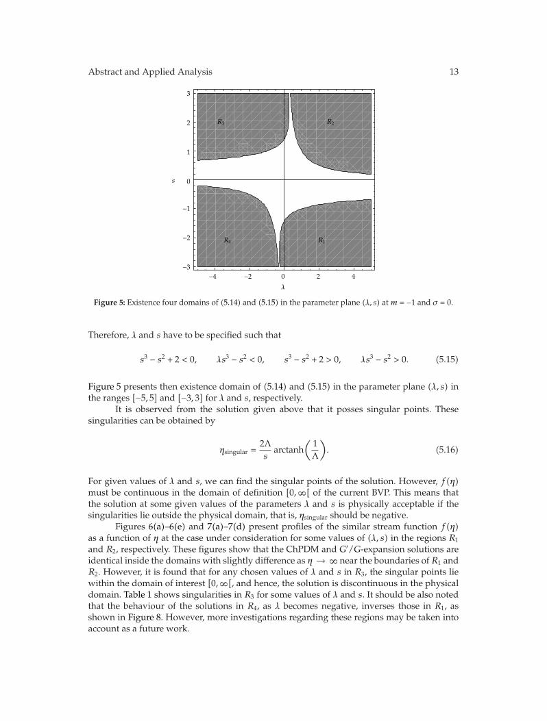
Figure 5: Existence four domains of (5.14) and (5.15) in the parameter plane (λ, s) at m = −1 and σ = 0.

Therefore, λ and s have to be specified such that

s3 − s2 + 2 < 0, λs3 − s2 < 0, s3 − s2 + 2 > 0, λs3 − s2 > 0. (5.15)

Figure 5 presents then existence domain of (5.14) and (5.15) in the parameter plane (λ, s) inthe ranges [−5, 5] and [−3, 3] for λ and s, respectively.

It is observed from the solution given above that it posses singular points. Thesesingularities can be obtained by

ηsingular =2Λs

arctanh(

1Λ

). (5.16)

For given values of λ and s, we can find the singular points of the solution. However, f(η)must be continuous in the domain of definition [0,∞[ of the current BVP. This means thatthe solution at some given values of the parameters λ and s is physically acceptable if thesingularities lie outside the physical domain, that is, ηsingular should be negative.

Figures 6(a)–6(e) and 7(a)–7(d) present profiles of the similar stream function f(η)as a function of η at the case under consideration for some values of (λ, s) in the regions R1

and R2, respectively. These figures show that the ChPDM and G′/G-expansion solutions areidentical inside the domains with slightly difference as η → ∞ near the boundaries of R1 andR2. However, it is found that for any chosen values of λ and s in R3, the singular points liewithin the domain of interest [0,∞[, and hence, the solution is discontinuous in the physicaldomain. Table 1 shows singularities in R3 for some values of λ and s. It should be also notedthat the behaviour of the solutions in R4, as λ becomes negative, inverses those in R1, asshown in Figure 8. However, more investigations regarding these regions may be taken intoaccount as a future work.


0 1 2 3 4η

−2.5−2.4−2.3−2.2−2.1−2

−1.9

f(η)

(a)

0 1 2 3 4 5 6

η

−2−1.95−1.9−1.85−1.8−1.75

f(η)

(b)

−3

−2.98

−2.96

−2.94

−2.92

f(η)

0 1 2 3 4 5 6 7

η

(c)

0 1 2 3 4 5 6η

−2−1.98−1.96−1.94−1.92−1.9

f(η)

(d)

0 1 2 3 4 5 6 7η

−1

−0.95

−0.9

−0.85

f(η)

(e)

Figure 6: Profiles of the similar stream function f(η) as a function of η at m = −1, σ = 0 in R1 for (a)λ = −0.1 and s = −2.5, (b) λ = 0.5 and s = −2, (c) λ = 1 and s = −3, (d) λ = 2 and s = −2, and (e) λ = 5 ands = −1, where solid and dashed lines are for ChPDM and G′/G-expansion solutions, respectively.

(2) When σ /= 0.

Using the first two boundary conditions to the solution given by (4.10) yields

σ − 4μ

σ −√σ2 − 4μ tanh

(η0) = s, (5.17)

(σ cosh

(η0) −

√σ2 − 4μ sinh(η0)

)3

= 2μ(4μ − σ2

)[(σ + 4λμ − λσ2

)cosh

(η0)+ (λσ − 1)

√σ2 − 4μ sinh

(η0)].

(5.18)


0 1 2 3 4 5η

−1.5−1

−0.50

0.5

1

f(η)

(a)

0 1 2 3 4 5 6 7η

2

1

0

−1

−2

f(η)

(b)

0 2 4 6 8

η

1

0.5

0

−0.5

−1

f(η)

(c)

0 1 2 3 4 5 6

η

3

2

1

0

−1−2−3

f(η)

(d)

Figure 7: Profiles of the similar stream function f(η) as a function of η at m = −1, σ = 0 in R2 for (a) λ = 2and s = 1, (b) λ = 3 and s = 2, (c) λ = 4 and s = 1, and (d) λ = 5 and s = 3, where solid and dashed linesare for ChPDM and G′/G-expansion solutions, respectively.

0 1 2 3 4 5 6

η

−2.15

−2.1

−2.05

−2

−1.95

−1.9

f(η)

R1

R4

λ = 2, s = −2

λ = −2, s = −2

Figure 8: Profiles of the similar stream function f(η) as a function of η atm = −1, σ = 0 in R1, for λ = 2 ands = −2, and R4, for λ = −2 and s = −2, where solid and dashed lines are for ChPDM and G′/G-expansionsolutions, respectively.

By solving (5.17) for η0, we get

η0 = tanh−1

⎛

⎜⎝

σ(s − σ) + 4μ

(s − σ)√σ2 − 4μ

⎞

⎟⎠. (5.19)


Table 1: Some values of λ and swith their singularities in R3.

λ s ηsingular

0.2 2 1.160.1 3 0.95−0.1 2 1.32−0.1 3 1.12−1 2 1.69−3 2 2.07−4 1 2.66

By substituting η0 from (5.19) into (5.18) and solving the resulted equation for σ, we obtain

σ = ±√

λs3 − s2 + 2 + 4μ(λs − 1)λs − 1

. (5.20)

Therefore, the exact solution in this case, m = −1, is given by f(η) in (4.10), where η0 and σare defined by (5.19) and (5.20), respectively. This solution can be easily checked by a directsubstitution.

Case 4 (a fractional m). Proceeding as above, we obtain the following equations fromapplying the first two boundary conditions to the solution f(η) in (4.11):

6σC2

(2m − 1)(C1σ − 2C2)= s, (5.21)

(2m − 1)(C1σ − 2C2)3 = 6σ2C22[σC1 + 2(λσ − 1)C2]. (5.22)

By solving (5.21) for C1 and substituting the result into f(η) in (4.11) and (5.22), then thefollowing exact solution can be derived:

f(η)=

6s6 + (2m − 1)sη

, (5.23)

provided that m, λ, and s are related by the equation

λ(2m − 1)2s3 + 3(2m − 1)s2 + 18 = 0. (5.24)

The solution given by (5.23) and (5.24) can be also checked by a direct substitution.

Lemma 5.2. From (5.24), it is observed that λ > 0 at the following cases:

(i) at 0 < m < 1/2 when s ∈]√−6/(2m − 1),∞[,

(ii) at m > 1/2 when s < 0,

(iii) at m < 0 when s ∈]√6/(1 − 2m),∞[∪] −

√6/(1 − 2m), 0[.


Proof. On solving (5.24) for λ, we then get

λ = −3(2m − 1)s2 + 18

(2m − 1)2s3. (5.25)

(i) At 0 < m < 1/2, this leads to 3(2m − 1)s2 < 0. Now setting 3(2m − 1)s2 + 18 < 0,we obtain s2 > −6/(2m− 1), that is, s ∈]−∞,−

√−6/(2m − 1)[

⋃]√−6/(2m − 1),∞[.

However, s ∈] −∞,−√−6/(2m − 1)[⇒ λ < 0 and s ∈]

√−6/(2m − 1),∞[⇒ λ > 0.

(ii) When m > 1/2, this means that 3(2m − 1)s2 + 18 >, for all s ∈ �. In this case, thedenominator in (5.25) should be negative so that λ > 0. Hence, s must be negativereal number, that is, s < 0.

(iii) Here, we may rewrite λ in (5.25) as

λ =3(1 − 2m)s2 − 18

(2m − 1)2s3. (5.26)

At m = 0, we note that 3(1 − 2m)s2 > 0. Therefore, λ is positive if the numerator anddenominator have the same sign, that is, the following conditions have to be held:

3(1 − 2m)s2 − 18 > 0, s > 0, 3(1 − 2m)s2 − 18 < 0, s < 0. (5.27)

On solving the inequalities in (5.27), we obtain the range of s as

s ∈⎤

⎦

√6

1 − 2m,∞

⎡

⎣⋃

⎤

⎦−√

61 − 2m

, 0

⎡

⎣. (5.28)

5.1. Important Remark: G′/G-Expansion Method Over the Others

Here, we aim to show that the exact solutions obtained in the previous subsections cannotbe achieved by using some other methods. Ebaid [18] pointed out that the Jacobi-ellipticfunction and F-expansion methods cannot be used to search the exact solutions for nonlineardifferential equations that include both odd and even-order derivative terms. However,He indicated the applicability of the standard exp-function method to solve such kind ofequations. Despite this ability, on applying the exp-function method [17] to solve (1.1) and(1.2), it does not provide any of the exact solutions obtained by the current method. To clarifythis point, this method is applied to the present BVP when m = 1, and the results are foundas

f(η)= 1 − (1 − s)e−η, (5.29)


where λ and s are governed by the following equation:

λ(1 − s) − s = 0 or λ =s

1 − s, s /= 1. (5.30)

In view of (5.29), the solution is trivial at s = 1. In the case of λ > 0, this exact solution isphysically acceptable in a very short range for the parameter (s ∈ [0, 1[). The solution givenby (5.29) and (5.30) is therefore just a special case of that obtained by generalized G′/G-expansion method and given by (5.5) and (5.6). The same conclusion can be also deducedwhen applying the standard exp-function method at m = −1. Moreover, the rest of solutionsgiven by (5.10) and (5.11) (at m = 0) and (5.23) and (5.24) cannot be recovered by using theexp-function method. In view of this discussion, it may be concluded that the generalizedG′/G-expansion method has many advantages over the exp-function method for the presentBVP. Further, in order to make this point as clear as possible, an appendix containing themathematical details of applying the exp-function method to the current problem is added.

6. Solution for 0 < λ 1

In the view of Aly et al. [34], the main attention is paid to the construction of solutions for(1.1) and (1.2), when λ → 0. We look for a solution which has the form

f(η)= f0 + λf1 + · · · . (6.1)

Substituting (6.1) into (1.1) and (1.2), we obtain the equations

f ′′′0 + λf ′′′

1 +m(f0 + λf1

)(f ′′0 + λf ′′

1

) − (f ′0 + λf ′

1

)2 = 0,

f0(0) + λf1(0) +O(λ2)= s,

f ′0(0) + λf ′

1(0) +O(λ2)= 1 + λ

[f ′′0 (0) + λf ′′

1 (0) +O(λ2)]

,

f ′0(∞) + λf ′

1(∞) +O(λ2)= 0.

(6.2)

We obtain at λ0

f ′′′0 +mf0f

′′0 − (

f ′0)2 = 0,

f0(0) = s, f ′0(0) = 1, f ′

0(∞) = 0,(6.3)

where at λ1, we get

f ′′′1 +m

(f0f

′′1 + f1f

′′0) − 2f ′

0f′1 = 0,

f1(0) = 0, f ′1(0) = f ′′

0 (0), f ′1(∞) = 0.

(6.4)


Equation (6.3) appears in the study of similarity solutions to problems of boundary-layertheory in some contexts of fluid mechanics, see, for example, [26, 27, 33, 34]. Exact solutionsfor these equations can be easily found, for different values of m, by applying the techniquein Section 5. We substitute then this solution in the system (6.4) to get the construction of f1.This means that the form of f(η) can be therefore evaluated by (6.1).

7. Asymptotic Solution (λ � 1)

As in [26] and by means of a shooting method, the boundary condition at infinity is replacedby the condition

f ′′(0) = α, (7.1)

where α is the shooting parameter which has to be determined. Regarding the difficulties ofobtaining the numerical solution of the system (1.1) and (1.2) in the case of λ � 1 and asin [26, 27, 34], we now seek a new set of full equations which do not contain λ on using thefollowing transformation:

f(η)= η + εϑH(ζ) where ζ = εγη, (7.2)

where ε = λα; ϑ and γ are constants to be determined. On substituting expressions (7.2) into(1.1), we obtain

ε2γH ′′′ + εγmηH ′′ + εϑ+γ[mHH ′′ −H

′2]− 2H ′ − ε−ϑ = 0. (7.3)

In order to ensure that the highest derivative remains present in the resulting equation, soavoiding the need to disregard any of the boundary conditions, we look for a balance withinthe equation of this term. Hence, we obtain ϑ = γ = 1/2. Therefore, when ε → ∞ (i.e.,λ → ∞), we obtain the following new set of full equations:

H ′′′ +mHH ′′ −H′2 = 0, (7.4)

H(0) = 0, H ′(0) = 1, H ′′(0) = 0. (7.5)

The boundary conditions (7.5) do not contain ε. As in the last section, (7.4) and (7.5) can besolved by meaning of Section 5.

8. Conclusion

Third-order nonlinear differential equations describing the nano boundary-layer flow havebeen investigated theoretically, using G′/G-expansion method, and numerically, applyingChPDM approach. The present results are itemized as follows.

(i) It is found that the ChPDM results are very accurate in an excellent manner oncomparing to those published in the literature using the homotopy analysis methodand the modified differential transform-Pade method.


(ii) For the first time, we have showed the way of applying G′/G-expansion method tosolve nonlinear BVPs. In addition, it has been proven that it has many advantagesover some of the other methods on solving the present BVP, where four certaindomains for the physical parameters have been discussed.

(iii) ChPDM technique has been successfully applied to validate and evidence theresulted exact solutions, for different positive and negative values of the investi-gated parameters, m, s, and λ.

(iv) Convex solutions have been obtained atm = 1 in the special case of λf ′′(0) = −2.(v) Vicinity of zero and asymptotic solutions when 0 < λ 1 and λ � 1, respectively,

are also deduced. It should be noted that, in both cases, λ does not exist. Therefore,the resulting equations are easy to deal with analytically and numerically.

Appendix

In this section, details of applying the exp-function method to the investigated problem (1.1)and (1.2) are introduced. The aim is to confirm that the solution obtained through this methodgiven by (5.26) and (5.27) is in fact a special case of the exact one obtained by using theG′/G-expansion method. Very recently, Ebaid [35] proved that on searching for exact solution byusing the exp-function method, one can go directly by assuming the solution in the form:

f =a0 + a1 exp

[η]+ a−1 exp

[−η]

b0 + b1 exp[η]+ b−1 exp

[−η] , (A.1)

where the tedious calculations of the balancing procedure are not required. On substituting(A.1) into (1.1), multiplying by (b1eη + e−ηb−1 + b0)

4, and then equating the coefficients ofeach exp-function to zero, we obtain the following system of algebraic equations:

2(2(−1 +m)a2

−1b21 + b−1

(2(−1 +m)a21b−1 + (1 − 3m)a2

0b1 + a1(2 + (−1 +m)a0 − 16b−1b1)))

+ 2(a−1(b1(−2 + (−1 +m)a0 + 16b−1b1) + a1(1 +m − 4(−1 +m)b−1b1))) = 0,

(−4 + 3m)a21b−1 + b1(−a0(1 +ma0) + (a−1(−5 + (−4 + 5m)a0) + 23a0b−1)b1)

+ a1(1 +ma0 + 2((2 +m)a−1 + (−9 + (2 − 5m)a0)b−1)b1) = 0,

(−4 + 3m)a2−1b1 + a−1(−1 + 2b−1((2 +m)a1 + 9b1) + a0(m + 2(2 − 5m)b−1b1))

+ b−1(5a1b−1 − a0(−1 +ma0 + b−1((4 − 5m)a1 + 23b1))) = 0,

b21(a0(4 + (−1 +m)a0) − 8a−1b1) + a21(−1 +m − 4mb−1b1)

+ 2a1b1(−2 − (−1 +m)a0 + 2(ma−1 + 2b−1)b1)b2−1(a0(−4 + (−1 +m)a0) + 8a1b−1)

+ 2a−1b−1(2 − (−1 +m)a0 + 2b−1(ma1 − 2b1)) + a2−1(−1 +m − 4mb−1b1) = 0,

b1(ma1 − b1)(a1 − a0b1) = 0,

b−1(ma−1 + b−1)(a−1 − a0b−1) = 0.

(A.2)


On solving this system, we obtain a nontrivial solution at m = 1 as

a0 = a−1b1 + 1, a1 = b1, b−1 = 0, f = 1 + e−ηa−1. (A.3)

On applying the first boundary condition, we obtain a−1 = s − 1. The exact solution hencebecomes

f = 1 − (1 − s)e−η, (A.4)

which is equivalent to (5.29). Now on applying the second boundary condition, this leadsdirectly to (5.30).

In conclusion, the above discussion shows that application of the exp-function methodto the present problem gives the same solution in (5.29) and (5.30)which is already shown inSection 5.1. Exp-function method came therefore as a special case from one of the solutionsprovided by the G′/G-expansion method.

Acknowledgment

This paper was funded by the Deanship of Scientific Research (DSR), King AbdulazizUniversity, Jeddah, under Grant no. (105-130-D1432). The authors, therefore, acknowledgewith thanks DSR technical and financial support.

References

[1] J.-H. He, Y.-Q. Wan, and L. Xu, “Nano-effects, quantum-like properties in electrospun nanofibers,”Chaos, Solitons and Fractals, vol. 33, no. 1, pp. 26–37, 2007.

[2] L. Prandtl, “Uber Flussigkeitsbewegung bei sehr kleiner Reibung,” in Proceedings of the 3rd Interna-tional Mathematical Congress, 1904.

[3] M. Gad-el-Hak, “The fluid mechanics of macrodevices-the Freeman scholar lecture,” Journal of FluidsEngineering, vol. 121, pp. 5–33, 1999.

[4] M. T. Matthews and J. M. Hill, “Nano boundary layer equation with nonlinear Navier boundarycondition,” Journal of Mathematical Analysis and Applications, vol. 333, no. 1, pp. 381–400, 2007.

[5] M. T. Matthews and J. M. Hill, “Micro/nano thermal boundary layer equations with slip-creep-jumpboundary conditions,” IMA Journal of Applied Mathematics, vol. 72, no. 6, pp. 894–911, 2007.

[6] M. T. Matthews and J. M. Hill, “A note on the boundary layer equations with linear slip boundarycondition,” Applied Mathematics Letters, vol. 21, no. 8, pp. 810–813, 2008.

[7] J. Cheng, S. Liao, R. N. Mohapatra, and K. Vajravelu, “Series solutions of nano boundary layer flowsby means of the homotopy analysis method,” Journal of Mathematical Analysis and Applications, vol.343, no. 1, pp. 233–245, 2008.

[8] C. Y. Wang, “Analysis of viscous flow due to a stretching sheet with surface slip and suction,”Nonlinear Analysis. Real World Applications, vol. 10, no. 1, pp. 375–380, 2009.

[9] F. Talay Akyildiz, H. Bellout, K. Vajravelu, and R. A. Van Gorder, “Existence results for third ordernonlinear boundary value problems arising in nano boundary layer fluid flows over stretchingsurfaces,” Nonlinear Analysis. Real World Applications, vol. 12, no. 6, pp. 2919–2930, 2011.

[10] M. M. Rashidi and E. Erfani, “The modified differential transform method for investigating nanoboundary-layers over stretching surfaces,” International Journal of Numerical Methods for Heat & FluidFlow, vol. 21, pp. 864–883, 2011.

[11] R. A. Van Gorder, E. Sweet, and K. Vajravelu, “Nano boundary layers over stretching surfaces,” Com-munications in Nonlinear Science and Numerical Simulation, vol. 15, no. 6, pp. 1494–1500, 2010.

[12] C. Y. Wang, “Flow due to a stretching boundary with partial slip-an exact solution of the Navier-Stokes equations,” Chemical Engineering Science, vol. 57, pp. 3745–3747, 2002.


[13] E. J. Parkes and B. R. Duffy, “An automated tanh-function method for finding solitary wave solutionsto nonlinear evolution equations,” Computer Physics Communications, vol. 98, pp. 288–300, 1996.

[14] S. Liu, Z. Fu, S. Liu, and Q. Zhao, “Jacobi elliptic function expansion method and periodic wavesolutions of nonlinear wave equations,” Physics Letters A, vol. 289, no. 1-2, pp. 69–74, 2001.

[15] A. Ebaid and E. H. Aly, “Exact solutions for the transformed reduced Ostrovsky equation via the F-expansion method in terms of Weierstrass-elliptic and Jacobian-elliptic functions,” Wave Motion, vol.49, pp. 296–308, 2012.

[16] J.-H. He and X.-H.Wu, “Exp-function method for nonlinear wave equations,” Chaos, Solitons and Frac-tals, vol. 30, no. 3, pp. 700–708, 2006.

[17] X.-H. Wu and J.-H. He, “EXP-function method and its application to nonlinear equations,” Chaos,Solitons and Fractals, vol. 38, no. 3, pp. 903–910, 2008.

[18] A. Ebaid, “Exact solitary wave solutions for some nonlinear evolution equations via Exp-functionmethod,” Physics Letters A, vol. 365, no. 3, pp. 213–219, 2007.

[19] A. Ebaid, “Application of the exp-function method for solving some evolution equations with non-linear terms of any orders,” Zeitschrift fur Naturforschung, vol. 65, pp. 1039–1044, 2010.

[20] C. Chun, “New solitary wave solutions to nonlinear evolution equations by the Exp-functionmethod,” Computers & Mathematics with Applications, vol. 61, no. 8, pp. 2107–2110, 2011.

[21] A. Ebaid, “Generalization of He’s exp-function method and new exact solutions for Burgers equa-tion,” Zeitschrift fur Naturforschung, vol. 64, pp. 604–608, 2009.

[22] M. Wang, X. Li, and J. Zhang, “The G′/G-expansion method and travelling wave solutions of non-linear evolution equations in mathematical physics,” Physics Letters A, vol. 372, no. 4, pp. 417–423,2008.

[23] R. Abazari, “Application of G′/G-expansion method to travelling wave solutions of three nonlinearevolution equation,” Computers & Fluids, vol. 39, no. 10, pp. 1957–1963, 2010.

[24] S. Yu, “A generalized G′/G-expansion method and its application to the MKdV equation,” Interna-tional Journal of Nonlinear Science, vol. 8, no. 3, pp. 374–378, 2009.

[25] X. Fan, S. Yang, and D. Zhao, “Travelling wave solutions for the Gilson-Pickering equation by usingthe simplified G′/G-expansion method,” International Journal of Nonlinear Science, vol. 8, no. 3, pp.368–373, 2009.

[26] E. H. Aly, M. Benlahsen, and M. Guedda, “Similarity solutions of a MHD boundary-layer flow past acontinuous moving surface,” International Journal of Engineering Science, vol. 45, no. 2–8, pp. 486–503,2007.

[27] M. Guedda, E. H. Aly, and A. Ouahsine, “Analytical and ChPDM analysis of MHDmixed convectionover a vertical flat plate embedded in a porousmedium filled with water at 4◦C,”AppliedMathematicalModelling, vol. 35, no. 10, pp. 5182–5197, 2011.

[28] E. H. Aly, N. T. El-Dabe, and A. S. Al-Bareda, “ChPDM analysis for MHD flow of viscoelastic fluidthrough porous media,” Journal of Applied Sciences Research. In press.

[29] L. J. Crane, “Flow past a stretching plate,” Zeitschrift fur Angewandte Mathematik und Physik, vol. 21,pp. 645–647, 1970.

[30] H. I. Andersson, “Slip flow past a stretching surface,” Acta Mechanica, vol. 158, pp. 121–125, 2002.[31] P. S. Gupta and A. S. Gupta, “Heat and mass transfer on a stretching sheet with suction or blowing,”

The Canadian Journal of Chemical Engineering, vol. 55, pp. 744–746, 1977.[32] T. Fang, S. Yao, J. Zhang, and A. Aziz, “Viscous flow over a shrinking sheet with a second order slip

flow model,” Communications in Nonlinear Science and Numerical Simulation, vol. 15, no. 7, pp. 1831–1842, 2010.

[33] B. Brighi and J.-D. Hoernel, “Similarity solutions for high frequency excitation of liquid metal in anantisymmetric magnetic field,” in Self-Similar Solutions of Nonlinear PDE, vol. 74, pp. 41–57, PolishAcademy of Science, Warsaw, Poland, 2006.

[34] E. H. Aly, L. Elliott, and D. B. Ingham, “Mixed convection boundary-layer flow over a vertical surfaceembedded in a porous medium,” European Journal of Mechanics B, vol. 22, no. 6, pp. 529–543, 2003.

[35] A. Ebaid, “An improvement on the exp-function method when balancing the highest order linear andnonlinear terms,” Journal of Mathematical Analysis and Applications, vol. 392, pp. 1–5, 2012.

Documents

On the Exact Analytical and Numerical Solutions of Nano