On the Existence and Uniqueness of Trade Equilibria∗

Treb Allen

Northwestern and NBER

Costas Arkolakis

Yale and NBER

Xiangliang Li

Yale and NSD, PKU

First Draft: April 2015

This Version: July 2015

PRELIMINARY AND INCOMPLETE

Abstract

We prove a number of new theorems that offer sufficient conditions for the existence

and uniqueness of equilibrium systems. The theorems are powerful: we show how they

can be applied to drastically simplify existing proofs for well known equilibrium systems

and establish results for systems not previously characterized. We first present a new

results concerning the existence, uniqueness, and calculation of a class of models where

economic interactions between agents are subject to potentially many sets of bilateral

frictions. We then offer a generalization of the gross substitutes condition that can

be applied recursively to offer the proofs of existence and/or uniqueness for general

equilibrium systems too complicated to be tackled using existing methods. We illustrate

the power of this method by providing (for the first time) sufficient conditions for the

existence and uniqueness of two well known trade models: a multi-country monopolistic

competition model with heterogenous firms and a (nearly) arbitrary distribution of firm

productivities in each country, and of a perfect competition setup with intermediate

inputs and input-output relationships.

∗We thank Pol Antras, Lorenzo Caliendo and Dave Donaldson. All errors are our own.

1

1 Introduction

In recent years, there has been a rapid proliferation of “quantitative” general equilibrium

models. These models are general equilibrium systems that include a large number of pa-

rameters and a large number of equilibrium outcomes to make them sufficiently flexible to be

applied empirically to understand real world economic systems (e.g. trade across many loca-

tions, the economic distribution of activity across space, the internal structure of cities, etc.).

While there has been much success in incorporating increasingly sophisticated economic in-

teractions within these models, the understanding of the general equilibrium properties of the

models themselves has lagged behind. Understanding these general equilibrium properties,

however, is of paramount importance; for example, the comparative statics of quantitative

models are well defined only if the equilibrium of that model exists and is unique. In this

paper, we provide a number of new mathematical results to facilitate the understanding of

these two important properties.

We first consider a particular form of general equilibrium systems that are common

in the spatial economics literature where equilibrium outcomes of one economic agent are

(loosely speaking) “weighted averages” of the equilibrium outcomes of other economic agents,

where the “weights” are determined by exogenous bilateral frictions.1 We provide a new

theorem that provides sufficient conditions for existence and uniqueness of such systems for

an any number of endogenous variables and any number of (arbitrary) bilateral frictions.

Furthermore, we provide an algorithm for calculating such an equilibrium and sufficient

conditions under which the algorithm will converge. Finally, we prove that the sufficient

conditions for uniqueness are also necessary, in the sense that if they are not satisfied, then

there exists some bilateral trade frictions (i.e. some“geography”) such that multiple equilibria

will arise.

We next consider the general form of general equilibrium systems. Much like Blackwell’s

sufficient conditions for a contraction mapping, these sufficient conditions are meant to be

easily verifiable. For existence, the sufficient conditions require one suitably well behaved

operator corresponding to the equilibrium system of study and guarantee that Brouwer’s

fixed point theorem can be applied. For uniqueness, the sufficient conditions generalize the

“gross substitutes” conditions of Mas-Colell, Whinston, and Green (1995) by relaxing the

homogeneity of degree zero assumption. We then show that these conditions can be applied

recursively, allowing one to break up complicated general equilibrium systems into more

manageable pieces.

1See Allen and Arkolakis (2014) for how these systems arise in economic geography models and Allen,Arkolakis, and Takahashi (2014) for how they arise in trade models exhibiting gravity.

2

To illustrate the power of the method, we tackle a problem that has vexed trade economists

for more than a decade: is the Melitz (2003) model well behaved for an arbitrary distribution

of firm productivity (and possibly varying across countries)? Reassuringly, it turns out that

the Melitz (2003) model is well behaved and both existence and uniqueness holds for (nearly)

any distribution of firm productivities. Similarly, we discuss existence and uniqueness in the

perfect competition setup of Eaton and Kortum (2002) with intermediate inputs and input-

output relationships, as formulated by Caliendo and Parro (2015). While existence in this

model holds generally, it turns out that the sufficient conditions for uniqueness place strong

restrictions on the form of the input-output linkages across countries.

This paper is organized as follows: in the next section, we present a new set of results

regarding the existence and uniqueness of equilibria with arbitrary bilateral frictions between

economic agents. In Section 3, we present the theorems providing the sufficient conditions

of existence and uniqueness for general equilibrium systems as well as offer several examples

of how these theorems can be applied. In Section 4, we show how these conditions can

be used to tackle the existence and uniqueness of more complicated general equilibrium

systems recursively and apply this algorithm to the Melitz (2003) model with arbitrary firm

productivity distributions and the Caliendo and Parro (2015) with input-output linkages

across sectors. Section 5 concludes.

2 Existence and uniqueness of “gravity” trade models

with many bilateral frictions

An important class of general equilibrium systems are those in which interactions between

economic agents are subject to bilateral frictions. For example, in “gravity” trade models,

it is assumed that the movement of goods between locations is subject to bilateral trade

frictions. In this class of models, the equilibrium system oftentimes can be written in a

form where (loosely stated), the equilibrium outcome for one country/location is a function

of a “weighted average” of the equilibrium outcomes of other countries/locations, where the

“weights” are functions of the bilateral frictions. In this section, we present new results on

the existence and uniqueness of such equilibrium systems, where there are one or many sets

of bilateral frictions.

Specifically, consider a model where the equilibrium can be represented as the following

system of equations:

3

H∏k=1

(xki)γkh = λk

J∑j=1

Kkij

H∏h=1

(xhj)βkh k = 1, 2, .., H (1)

In such a framework, there are J locations and H unknown J-vector of endogenous vari-

ables, and J systems of equations that relate a log-linear function of endogenous variables

in location i to the sum of a possibly different log-linear function of endogenous variables

across all other locations j, where the sum is weighted by a set of exogenous bilateral trade

frictions. The characteristic values λ1, λ2, ..., λH are endogenous scalars that balance the

overall level of two sides of equations. Notice that due to the homogeneity imbedded in this

equation, solving system 1 can be always decomposed into two steps: the first step is to

find the solution x ={xhj}

that makes two sides of the above equations parallel with each

other i.e. for any k ∈ {1, 2, ..., H},∑Jj=1K

kij

∏Hh=1(xhj )

βkh∏Hh=1(xki )

γkh are equal for all i; the second step

is to adjust the characteristic values of the two sides be equal. The main challenge is the

first step and can be analyzed generally. The second part usually can be solved by some

normalization conditions (e.g. the total resources constraint) or the special structure of the

coefficients {γkh, βkh} and depends on the specific context. Thus, in the following we will

mainly demonstrate the results for the first step and show the second step by some examples.

Denote Γ as the H × H matrix whose element(Γ)kh = γkh, i.e. Γ is the matrix of

exponents of the left hand side. Similarly, define B to be the H ×H matrix whose element

(B)kh = βkh, i.e. B is the matrix of exponents on the right hand side. The following theorem

characterizes the properties of an equilibrium defined by the system 1 as a function of these

two matrices.

Theorem 1. Consider the system of equations 1. Assume Γ is invertible (non-singular).

Define the matrix A ≡BΓ−1, the matrix Ap to be the matrix constructed by the absolute value

of the elements of A, i.e.(Ap)kh = |(A)kh|, and define ρ (Ap) as Ap’s largest eigenvalue (or

“spectral radius”). Then we have:

i) If Kkij > 0 for all k, i, j, there exists a strictly positive solution.

ii) If ρ (Ap) ≤ 1 and Kkij ≥ 0 for all k, i, j, then there is at most one strictly positive

solution (to-scale).

iii) If ρ (Ap) < 1 and Kkij > 0 for all k, i, j, the unique solution can be computed by a

simple iterative procedure.

iv) If ρ (Ap) > 1 and all elements of each column of A have the same sign, then there

exists a kernel{Kkij

}such that there are multiple strictly positive solutions, i.e. for some set

of frictions, the uniqueness conditions above are both necessary and sufficient.

4

Proof. Details are in the appendix.

Notice that the equation system 1 is more general than first glance, as we can transform

many existing system into the above form by some simple tricks. For example, we can

redefine some variables and also increase/replicate the number of equations such that we can

rescale the dimension of all sets of equations to be the same. In the following, we show by

an example this kind of transformation and also the application of above theorem 1.

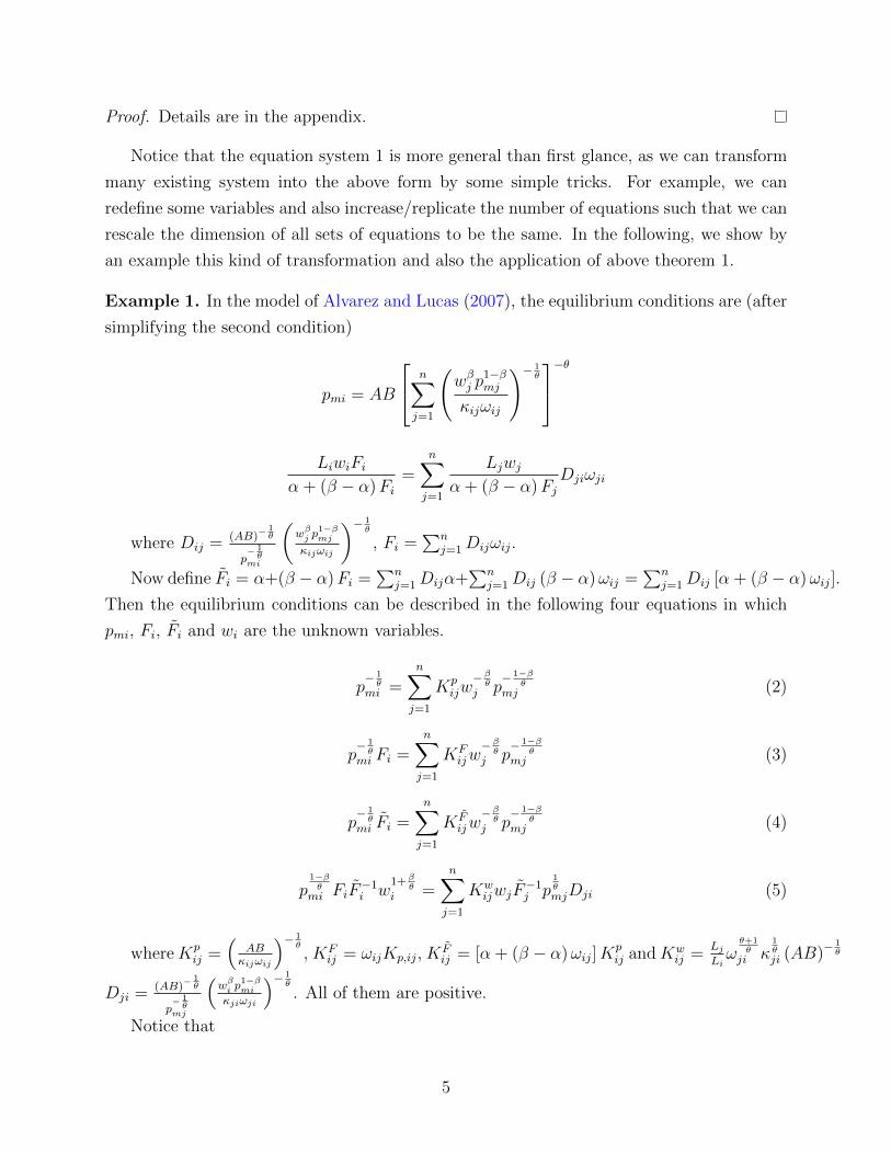
Example 1. In the model of Alvarez and Lucas (2007), the equilibrium conditions are (after

simplifying the second condition)

pmi = AB

n∑j=1

(wβj p

1−βmj

κijωij

)− 1θ

−θ

LiwiFiα + (β − α)Fi

=n∑j=1

Ljwjα + (β − α)Fj

Djiωji

where Dij = (AB)−1θ

p− 1θ

mi

(wβj p

1−βmj

κijωij

)− 1θ

, Fi =∑n

j=1Dijωij.

Now define Fi = α+(β − α)Fi =∑n

j=1 Dijα+∑n

j=1Dij (β − α)ωij =∑n

j=1Dij [α + (β − α)ωij].

Then the equilibrium conditions can be described in the following four equations in which

pmi, Fi, Fi and wi are the unknown variables.

p− 1θ

mi =n∑j=1

Kpijw−βθ

j p− 1−β

θmj (2)

p− 1θ

mi Fi =n∑j=1

KFijw−βθ

j p− 1−β

θmj (3)

p− 1θ

mi Fi =n∑j=1

K Fijw−βθ

j p− 1−β

θmj (4)

p1−βθ

mi FiF−1i w

1+βθ

i =n∑j=1

KwijwjF

−1j p

1θmjDji (5)

whereKpij =

(ABκijωij

)− 1θ, KF

ij = ωijKp,ij, KFij = [α + (β − α)ωij]K

pij andKw

ij =LjLiωθ+1θ

ji κ1θji (AB)−

1θ

Dji = (AB)−1θ

p− 1θ

mj

(wβi p

1−βmi

κjiωji

)− 1θ

. All of them are positive.

Notice that

5

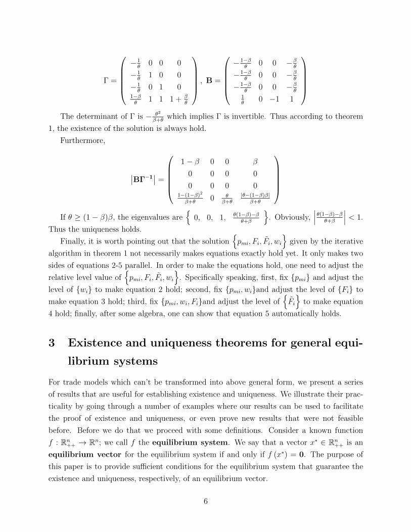
Γ =

−1θ

0 0 0

−1θ

1 0 0

−1θ

0 1 01−βθ

1 1 1 + βθ

, B =

−1−β

θ0 0 −β

θ

−1−βθ

0 0 −βθ

−1−βθ

0 0 −βθ

1θ

0 −1 1

The determinant of Γ is − θ2

β+θwhich implies Γ is invertible. Thus according to theorem

1, the existence of the solution is always hold.

Furthermore,

∣∣BΓ−1∣∣ =

1− β 0 0 β

0 0 0 0

0 0 0 01−(1−β)2

β+θ0 θ

β+θ|θ−(1−β)β|

β+θ

If θ ≥ (1− β)β, the eigenvalues are

{0, 0, 1, θ(1−β)−β

θ+β

}. Obviously,

∣∣∣ θ(1−β)−βθ+β

∣∣∣ < 1.

Thus the uniqueness holds.

Finally, it is worth pointing out that the solution{pmi, Fi, Fi, wi

}given by the iterative

algorithm in theorem 1 not necessarily makes equations exactly hold yet. It only makes two

sides of equations 2-5 parallel. In order to make the equations hold, one need to adjust the

relative level value of{pmi, Fi, Fi, wi

}. Specifically speaking, first, fix {pmi} and adjust the

level of {wi} to make equation 2 hold; second, fix {pmi, wi}and adjust the level of {Fi} to

make equation 3 hold; third, fix {pmi, wi, Fi}and adjust the level of{Fi

}to make equation

4 hold; finally, after some algebra, one can show that equation 5 automatically holds.

3 Existence and uniqueness theorems for general equi-

librium systems

For trade models which can’t be transformed into above general form, we present a series

of results that are useful for establishing existence and uniqueness. We illustrate their prac-

ticality by going through a number of examples where our results can be used to facilitate

the proof of existence and uniqueness, or even prove new results that were not feasible

before. Before we do that we proceed with some definitions. Consider a known function

f : Rn++ → Rn; we call f the equilibrium system. We say that a vector x∗ ∈ Rn

++ is an

equilibrium vector for the equilibrium system if and only if f (x∗) = 0. The purpose of

this paper is to provide sufficient conditions for the equilibrium system that guarantee the

existence and uniqueness, respectively, of an equilibrium vector.

6

3.1 Existence

We begin with existence and state the following lemma that provides relevant sufficient

conditions.

Lemma 1. Suppose there exists a once continuously differentiable “scaffold” function F :

Rn+1++ → Rn where for all i ∈ {1, ..., n}, fi (x) = Fi (x, xi) and the following conditions are

satisfied:

i) For all x′ ∈ Rn++ , there exists xi such that Fi (x

′, xi) = 0.

ii) ∂Fi(x′,xi)

∂xi

∂Fi(x′,xi)

∂x′j< 0 for all j.

iii) There exists x′ such that for xi defined in Fi (sx′, xi) = 0, xi = o (s) (i.e. when

s→∞ , sxi→∞ ; when s→ 0 , s

xi→ 0 ).

Then there exists an equilibrium vector x∗.

Proof. We proceed by using Brouwer’s fixed point theorem. From the first and second

condition, there exists a unique xi such that Fi (x′, xi) = 0. Thus we define the operator

T : x′ → x where xi satisfies Fi(x′, xi)

= 0. Thus we can also write equation F (sx′, xi) = 0

as xi = T (sx′). As s → ∞ implies sxi→ ∞, we can select a large enough M > 0 such that

for all i xi ≤ Mx′i i.e. x ≤ Mx′. Similarly, we can select a small enough m > 0 such that

x ≥ mx′. Now define K = {x|mx′ ≤ x ≤Mx′}.According to the second condition, we know that T (x) increases with respect to x thus

for any x ∈ K we have T (x) ∈ K. Thus, T : K → K. As a result, we can apply Brouwer’s

fixed point theorem, which guarantees existence.

Theorem 1 provides sufficient conditions under which one can construct a continuous

operator on a compact space whose fixed point corresponds to the equilibrium vector of the

considered equilibrium system. If these conditions hold, Brouwer’s fixed point theorem guar-

antees the existence of such a fixed point and hence the existence of an equilibrium vector.

The power of Theorem 1 is that rather than trying to prove existence directly for the equilib-

rium system f as is typically done, existence is achieved via selecting the appropriate scaffold

function F (so-called because it is only temporarily necessary to construct the conditions of

uniqueness for the equilibrium system f), which implicitly defines a continuous operator T

where existence can be more easily proven.

Intuitively, the scaffold function takes as inputs an “input” vector x′ and “output” vector

x; condition (i) says that the scaffold function implicitly defines an operator that for any

“input”vector x′ returns the“output”vector such that the scaffold function returns a vector of

zeros. Condition (ii) is a sufficient condition for the scaffold function to generate a monotonic

increasing operator. Condition (iii) requires that for some input vector, the implicit operator

increases at less than a linear rate.

7

Below, we provide several examples of how the right choice of a scaffold function can

greatly simplify the proof of existence. The first example is to establish the existence of a

price vector, given wages, in the general equilibrium version of the Eaton and Kortum (2002)

model developed by Alvarez and Lucas (2007).

Example 2. The first example is the existence part of Theorem 1 Alvarez and Lucas (2007).

Consider the following functional:

p−θi =n∑j=1

(Kijw

βj p

1−βj

)−θ∀i ∈ {1, ..., n} , (6)

where θ > 0, Kij > 0 for all i, j ∈ {1, ..., n} and wj > 0 for all j ∈ {1, ...., n} are all given

positive model parameters. This functional represents the price index of a consumer and

here we treat wages, wi, as given. We prove the existence of a vector of strictly positive {pi}that satisfy equation (6).

Proof. We proceed by verifying the conditions of 1. We define the scaffold function

Fi (p′, p) =

(n∑j=1

(Kijw

βj

(p′

j

)1−β)−θ)− 1

θ

− pi.

Condition (i) obviously holds, as setting pi =

(∑nj=1

(Kijw

βj

(p′j

)1−β)−θ)− 1

θ

implies Fi (p′, p) =

0; because ∂Fi(p′,pi)

∂pi= −1, ∂Fi(p

′,pi)∂pj

> 0, condition (ii) also holds; also considering Fi (sp′, p),

implies pi � s1−β, i.e. pi = o (s) condition (iii) also holds. Hence, there exists a set of {pi}that satisfy equation (6).

The second example is derived from a perfect competition model with multiple countries,

multiple sectors and input-output relationships across sectors, developed by Caliendo and

Parro (2015). Further complications may arise in this case because of the varying degrees of

relationship between countries and sectors. However, the proof of existence is straightforward

in this case too.

Example 3. In Caliendo and Parro (2015), the price is determined in this equation P jn =

Aj[∑N

i=1 λji

(cjiκ

jni

)−θj]−1/θj

where cjn = δjnwγjnn

∏Jk=1

(P kn

)γk,jn , 0 < γjn, γk,jn < 1 and γjn +∑J

k=1 γk,jn = 1, δjn is a constant. In this equation, only the price P k

n is endogenous. The

larger complication of this price index versus the previous is the existence of multiple sectors

and the complicated input-output structure.

8

Proof. After substituting cji out, we then first transform it into

(P jn

)−θj= Aj

N∑i=1

λji

(δjiw

γjii

J∏k=1

(P ki

)γk,ji κjni

)−θj.

Like in the example 2, we proceed by verifying the conditions of Lemma 1. We define the

scaffold function

Fj,n

(P , P j

n

)= Aj

N∑i=1

λji

(δjiw

γjii

J∏k=1

(P ki

)γk,jiκjni

)−θj−(P jn

)−θj.

Condition (i) obviously holds since our definition of P jn implies Fj,n

(P , P j

n

)= 0; obviously

∂Fj,n(P ,P jn)∂P jn

> 0,∂Fj,n(P ,P jn)

∂Pki< 0, so that condition (ii) also holds; besides,

Fj,n

(sP , P j

n

)= Aj

N∑i=1

s−(1−γji )θjλji

(δjiw

γjii

J∏k=1

(P ki

)γk,jiκjni

)−θj−(P jn

)−θj,

implies P jn � sβj , where βj ∈

{1− γji |i = 1, ..., N

}so that βj ∈ (0, 1). This implies P j

n = o (s)

i.e. condition (iii) also holds. Hence, there exists a set of {P jn} that satisfy equation (11)

which completes the derivation.

3.2 Uniqueness

A standard approach to proving uniqueness of general equilibrium systems requires homo-

geneity of degree zero and gross substitution conditions as sufficient conditions (see, for

example, Mas-Colell, Whinston, and Green (1995), chapter 17). However, there are many

examples of equilibrium systems where directly proving gross substitution is difficult. Of-

tentimes in these systems, gross substitution can be shown for a subset of the full general

equilibrium system; however, requiring homogeneity of degree zero prevents one from con-

sidering the uniqueness of one portion of that system. In example 1 above, we considered

the existence of prices given a set of wages; if we were to examine the uniqueness of prices

given a set of wages, it is straightforward to see that the partial system is not homogeneous

of degree zero. In what follows, we show that the homogeneity of degree zero restriction can

be relaxed, which will allows us to apply gross substitutes separately to subsets of the full

equilibrium system, thereby greatly simplifying the task of proving uniqueness.

Let us make some additional definitions that will be useful for the analysis that follows.

We say a function f (x) satisfies gross substitution if for any j 6= i, ∂fi∂xj

> 0. We say that

9

a function is homogeneous of degree α if f(tx) = tαf (x) for all t > 0. With these basic

definitions, we can now proceed to state our main results for uniqueness and describe their

applications. In the following Theorems 2 and 3, we show that even if homogeneity holds

partly or jointly with other variables (the exact definition can be seen below), we can still

have uniqueness without requiring full homogeneity of the system, i.e. fi (tx) = tkfi (x).

The first theorem generalizes the full homogeneity condition into a less demanding partial

homogeneity requirement.

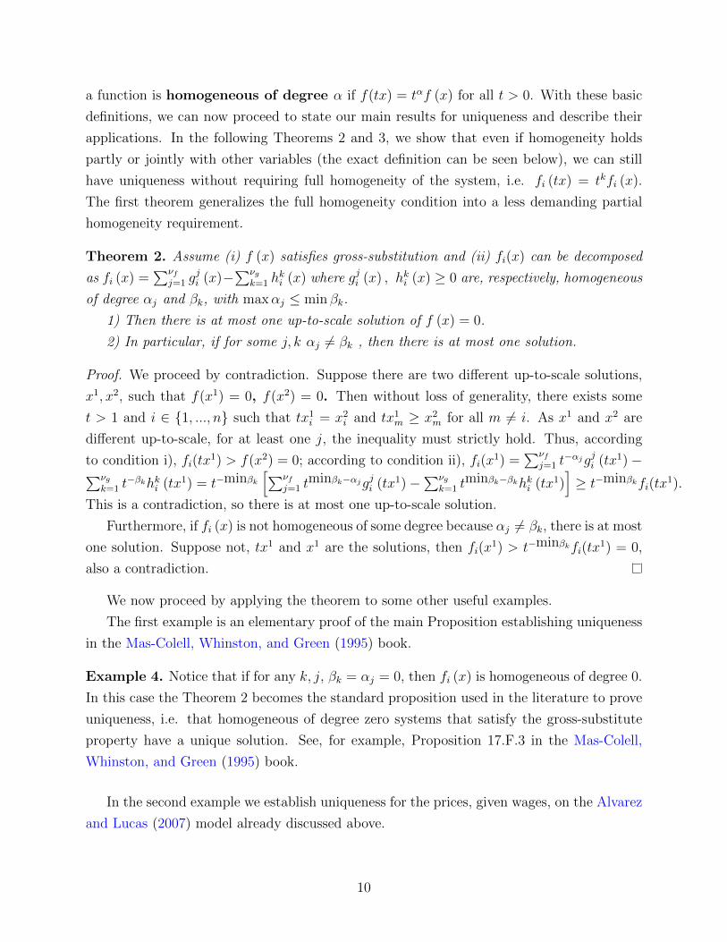
Theorem 2. Assume (i) f (x) satisfies gross-substitution and (ii) fi(x) can be decomposed

as fi (x) =∑νf

j=1 gji (x)−

∑νgk=1 h

ki (x) where gji (x) , hki (x) ≥ 0 are, respectively, homogeneous

of degree αj and βk, with maxαj ≤ min βk.

1) Then there is at most one up-to-scale solution of f (x) = 0.

2) In particular, if for some j, k αj 6= βk , then there is at most one solution.

Proof. We proceed by contradiction. Suppose there are two different up-to-scale solutions,

x1, x2, such that f(x1) = 0, f(x2) = 0. Then without loss of generality, there exists some

t > 1 and i ∈ {1, ..., n} such that tx1i = x2

i and tx1m ≥ x2

m for all m 6= i. As x1 and x2 are

different up-to-scale, for at least one j, the inequality must strictly hold. Thus, according

to condition i), fi(tx1) > f(x2) = 0; according to condition ii), fi(x

1) =∑νf

j=1 t−αjgji (tx1)−∑νg

k=1 t−βkhki (tx1) = t−minβk

[∑νfj=1 t

minβk−αjgji (tx1)−∑νg

k=1 tminβk−βkhki (tx1)

]≥ t−minβkfi(tx

1).

This is a contradiction, so there is at most one up-to-scale solution.

Furthermore, if fi (x) is not homogeneous of some degree because αj 6= βk, there is at most

one solution. Suppose not, tx1 and x1 are the solutions, then fi(x1) > t−minβkfi(tx

1) = 0,

also a contradiction.

We now proceed by applying the theorem to some other useful examples.

The first example is an elementary proof of the main Proposition establishing uniqueness

in the Mas-Colell, Whinston, and Green (1995) book.

Example 4. Notice that if for any k, j, βk = αj = 0, then fi (x) is homogeneous of degree 0.

In this case the Theorem 2 becomes the standard proposition used in the literature to prove

uniqueness, i.e. that homogeneous of degree zero systems that satisfy the gross-substitute

property have a unique solution. See, for example, Proposition 17.F.3 in the Mas-Colell,

Whinston, and Green (1995) book.

In the second example we establish uniqueness for the prices, given wages, on the Alvarez

and Lucas (2007) model already discussed above.

10

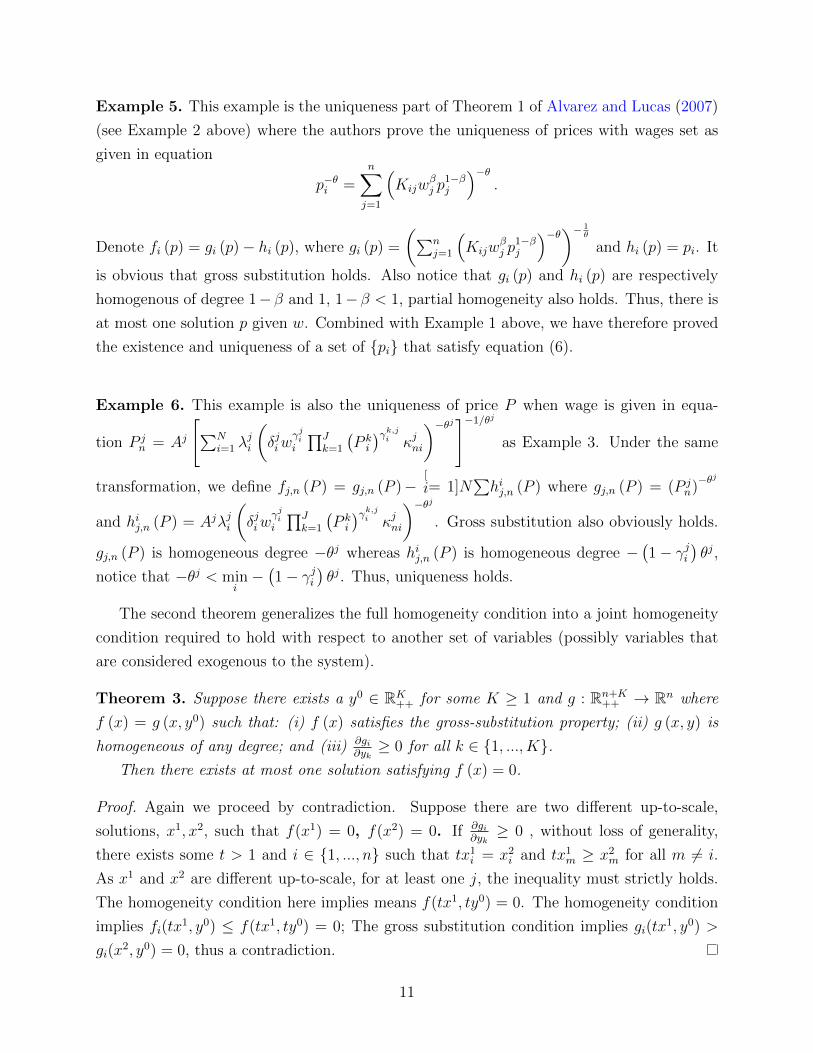
Example 5. This example is the uniqueness part of Theorem 1 of Alvarez and Lucas (2007)

(see Example 2 above) where the authors prove the uniqueness of prices with wages set as

given in equation

p−θi =n∑j=1

(Kijw

βj p

1−βj

)−θ.

Denote fi (p) = gi (p)− hi (p), where gi (p) =

(∑nj=1

(Kijw

βj p

1−βj

)−θ)− 1θ

and hi (p) = pi. It

is obvious that gross substitution holds. Also notice that gi (p) and hi (p) are respectively

homogenous of degree 1−β and 1, 1−β < 1, partial homogeneity also holds. Thus, there is

at most one solution p given w. Combined with Example 1 above, we have therefore proved

the existence and uniqueness of a set of {pi} that satisfy equation (6).

Example 6. This example is also the uniqueness of price P when wage is given in equa-

tion P jn = Aj

[∑Ni=1 λ

ji

(δjiw

γjii

∏Jk=1

(P ki

)γk,ji κjni

)−θj]−1/θj

as Example 3. Under the same

transformation, we define fj,n (P ) = gj,n (P )−[

i= 1]N∑hij,n (P ) where gj,n (P ) = (P j

n)−θj

and hij,n (P ) = Ajλji

(δjiw

γjii

∏Jk=1

(P ki

)γk,ji κjni

)−θj. Gross substitution also obviously holds.

gj,n (P ) is homogeneous degree −θj whereas hij,n (P ) is homogeneous degree −(1− γji

)θj,

notice that −θj < mini−(1− γji

)θj. Thus, uniqueness holds.

The second theorem generalizes the full homogeneity condition into a joint homogeneity

condition required to hold with respect to another set of variables (possibly variables that

are considered exogenous to the system).

Theorem 3. Suppose there exists a y0 ∈ RK++ for some K ≥ 1 and g : Rn+K

++ → Rn where

f (x) = g (x, y0) such that: (i) f (x) satisfies the gross-substitution property; (ii) g (x, y) is

homogeneous of any degree; and (iii) ∂gi∂yk≥ 0 for all k ∈ {1, ..., K}.

Then there exists at most one solution satisfying f (x) = 0.

Proof. Again we proceed by contradiction. Suppose there are two different up-to-scale,

solutions, x1, x2, such that f(x1) = 0, f(x2) = 0. If ∂gi∂yk≥ 0 , without loss of generality,

there exists some t > 1 and i ∈ {1, ..., n} such that tx1i = x2

i and tx1m ≥ x2

m for all m 6= i.

As x1 and x2 are different up-to-scale, for at least one j, the inequality must strictly holds.

The homogeneity condition here implies means f(tx1, ty0) = 0. The homogeneity condition

implies fi(tx1, y0) ≤ f(tx1, ty0) = 0; The gross substitution condition implies gi(tx

1, y0) >

gi(x2, y0) = 0, thus a contradiction.

11

Notice that Example 4 is a special case of Theorem 3 as well. We can also apply Theorem

3 in Example 5 if we choose wage wi as the joint variable. However, Theorems 1 and 2 are

not entirely substitutable. In the next section’s proof of the Melitz model only Theorem 3

can be used, as in that model we have changes in the extensive margin.

[More examples will be forthcoming.]

4 A general recipe for existence and uniqueness and

applications

So far, we have developed a set of sufficient conditions for the existence and uniqueness of

an equilibrium system. Unfortunately, general equilibrium models oftentimes are complex

systems comprising a large number of equations that are difficult to tackle simultaneously.

In this section, we show how the conditions developed in the previous section can be applied

recursively to subsets of the full equilibrium system, thereby simplifying the task of proving

existence and uniqueness. We then illustrate the power of this method by proving the

existence and uniqueness of several trade models: a multi-country monopolistic competition

model with heterogeneous firms, with an arbitrary distribution of firm productivities in each

country; a multi-sector model of Caliendo and Parro (2015).

4.1 The recipe: decompose the general equilibrium into a se-

quence of sub-problems

We formally state the procedure used in Alvarez and Lucas (2007) that decomposes the

general equilibrium problem into a sequence of sub-problems. Using the theorems devel-

oped above and below we can analyze one-by-one these problems and prove existence and

uniqueness, until we establish existence and uniqueness of the entire general equilibrium

system.

Specifically, suppose the general equilibrium system is defined by the equilibrium equa-

tions G (x) = 0 in which x is endogenous variable. The procedure to prove the existence and

uniqueness of solution x is as follows.

� Step 1: divide the equilibrium equations G and variables x into G1, ..., GP and x1, ...,xP

� Step 2: prove the existence and uniqueness of x1 in equations group G1 where x2, ...,xP

are taken as given. Then we denote x1 = G1(x2, ...,xP

)12

� Step 3: prove the existence and uniqueness of x2 in equations group G2 where x3, ...,xP

are taken as given and x1 = G1(x2, ...,xP

). Then we can denote x2 = G2

(x3, ...,xP

)� ...

� Step P : prove the existence and uniqueness of xP in equations group GP where xp−1 =

Gp−1(xP), ..., x1 = G1

(x2, ...,xP

). Q.E.D.

By proving the existence and uniqueness of various trade models, cases where these

properties have not been established so far, we will show that this can be a general way to

deal with general equilibrium problems with multiple groups of equations. However, there

are still several open issues left to deal with. For example, how we are going to rank the

equation groups and which variables should be taken as endogenous in the sub-problem?

The answer to those questions generally depends on the specific context of the model and no

rule-of-thumb can be provided. Instead, we present a number of examples to establish the

validity and practicality of the procedure.

Before proceeding into the examples, we first present a lemma which will be repeatedly

used in the following applications.

Lemma 2. Define S to be an n×n diagonal matrix with strictly positive diagonal elements,

i.e. sii > 0 for all i ∈ {1, .., n}. Define T to be a weakly positive n × n matrix (i.e. tij ≥ 0

for all i, j ∈ {1, ..., n}). Define n× n matrix A ≡ S−T.

1) If∑

j tij < sii, then A−1 exists and A−1 ≥ 0, A−1 =(I +

∑∞k=1 (S−1T)

k)

S−1.

Furthermore if T > 0, then A−1 > 0.

2) If∑

j tji < sii, the result is the same except A−1 = S−1(I +

∑∞k=1 (TS−1)

k)

.

Proof. Details is in the appendix.

We also present the following auxiliary lemma.

Lemma 3. Suppose A is a n× n positive matrix and λ0 is its positive eigenvalue. Then the

rank of λ0I−A is n− 1.

Proof. According to theorem 1 in page 53 of book Gantmakher (1959), λ0is a simple root

of |λI−A|, which means m0 = 1 in |λI−A| = (λ− λ0)m0 (λ− λ1)m1 . . . (λ− λk)mk where

λ0, λ1, . . . , λk are all the different eigenvalues of matrix A and∑mi = n. Then apparently

λ0 − λ0, λ1 − λ0, . . . , λk − λ0 is the eigenvalue of matrix λ0I − A, moreover |λI− (λ0I)| =

(λ− 0)m0 (λ− (λ1 − λ0))m1 . . . (λ− (λk − λ0))mk . Then the algebraic multiplicity of the non-

zero eigenvalue in matrix λ0I−A is n− 1, as a result, the rank of λ0I−A is n− 1 (see page

199 of book Ibe (2011)).

13

Having established the set of required results we proceed by establishing conditions for

existence and uniqueness in two well-known examples from the trade literature.

4.2 Heterogeneous firms with arbitrary country-specific produc-

tivity distributions

We consider a world of N countries. Each country has a measure Li of workers. Labor is the

only factor of production and worker’s wage is denoted by wi, and income per capita (that

maybe different than the wage) as yi. Total income is composed of labor income and profit

income, πi, and firm profits are equally distributed to local consumers. Consumers have

constant elasticity of substitution (CES) demand with respect to all varieties and elasticity

σ.

There is monopolistic competition and firms face variable and fixed costs of selling into

each market j. In particular, there is an iceberg cost τij of shipping the good from country

i to country j. In addition, firms pay a fixed exporting cost fij in terms of domestic labor

to sell to market j. Each firm has potentially different productivity and the density of firms

with productivity z is mi (z).

Notice that in this environment the marginal cost of a firm with productivity z of pro-

ducing its good in country i and selling to j is simply wiτij/z. Because of monopolistic

competition and CES demand function firms charge a constant markup over this marginal

cost so the corresponding price is given bypij (z) = σwiτijz.where σ = σ

σ−1. Given the above

assumption total sales of a firm z from country i in market j are simply

yij (z) =

(στijwiz

)1−σ

P 1−σj

yjLj.

In addition, gross profits, i.e. revenue minus production and shipping costs are simply

yij (z) /σ.

For brevity we omit most of the derivations that lead to the equilibrium conditions below

but briefly state the equilibrium conditions. For a discussion of the equilibrium conditions

and their detailed derivation see Melitz (2003), Arkolakis (2011) and Allen and Arkolakis

(2015). The general equilibrium of this economic environment is defined by the following

conditions: zero-profit for the cutoff firm, budget balance, labor market clearing and current

account balance. We describe each one in turn.

14

Zero profit condition: The zero-profit condition defines the productivity of the firm

from market i that exactly breaks even by selling to market j. Thus, the cutoff firm’s variable

profits in this market equal to its fixed marketing cost, i.e.

1

σyij(z∗ij)

= wifij,

so that cutoff productivity can be expressed as

z∗ij = cijw

σσ−1

i

Pjy1

σ−1

j

, (7)

where cij ≡ στij

[Ljσfij

] 11−σ

is a constant. At the same time, the sales revenue earned from

country j of firm z∗ij is σwifij. It is easy to show that the sales revenue earned from country

j between two different firms within the same country would be proportional to their pro-

ductivity ratio power to σ − 1. Thus the total revenue earned by country i from country j

is yij ≡ σwifij´∞z∗ij

(zz∗ij

)σ−1

mi(z)dz.

Budget Balance: The budget balance implies that the revenue earned by all firms from

country j should equal to its total expenditure yjLj, that is

yjLj =∑k

ykj. (8)

Labor market clearing: The labor market clearing condition implies that the total

labor income should equal to the sum of labor income from production and serving export

(e.g marketing)

wiLi =σ − 1

σ

∑j

yij +∑j

wifij

ˆ ∞z∗ij

mi(z)dz. (9)

Current account balance: The current account balance condition implies that the

total expenditure should equal to the total revenue.

yiLi =∑j

yij. (10)

An equilibrium in this setting is {yi, wi, Pi} such that equations 8, 9 and 10 hold. To

make the model meaningful, also for the purpose of proving uniqueness and existence, we

need the following condition.

15

Condition 1. Denote Gi(z∗) =

´∞z∗

(zz∗

)σ−1mi(z)dz. We assume that for any z∗ > 0, G(z∗)

is finite and strictly positive.

Condition 1 is the only restriction we place on the distribution of firm productivities in

each country. Note that this condition implies limz∗→∞

Gi(z∗) = 0 and lim

z∗→0Gi(z

∗) = ∞. Also

note that this condition holds for the Pareto distribution. Now we follow the above recipe

to decompose the equilibrium into a sequence of sub-problems and repeatedly use the above

theorems in each sub-problem. Specifically, we proceed in the following three steps.

� Step 1: prove the existence and uniqueness of {Pi} in equation (8) with {wi, yi} taken

as given.

� Step 2: prove the existence and uniqueness of {wi} in equation (9) with {yi} taken as

given and {Pi} endogenously solved in last step.

� Step 3: prove the existence and uniqueness of {yi} in equation (10) with {wi, Pi}endogenously solved in this last step.

The results of the above three steps can be summarized in the below theorem.

Proposition 1. Assume C.1 holds. Then there exists a unique (up-to-scale) {yi, wi, Pi}satisfying equations (8), (9) and (10).

Hence, the equilibrium of the many-country Melitz (2003) model is well defined (i.e. it

exists and is unique) for any set of country-specific distributions of firm productivities, as

long as those distributions satisfy Condition 1 above.

4.3 Multi-sector trade model with input-output linkages

The above theorems and the recipe to characterize the existence and uniqueness of an equi-

librium can also be applied in Caliendo and Parro (2015), a multi-country, multi-sector trade

model with input-output linkage among sectors.2 In Caliendo and Parro (2015), the equilib-

rium is defined by equations (2), (4), (6), (7), and (9). To facilitate the proof of existence and

uniqueness, the equilibrium conditions we use are slightly different from –but are equivalent

to– the equilibrium conditions in their paper.

The first equation is equation (4) in their paper, which defines price with wage given,

P jn = Aj

[N∑i=1

λji(cjiκ

jni

)−θj]−1/θj

, (11)

2Notice that in their paper, as in Dekle, Eaton, and Kortum (2008), there is nominal exogenous tradedeficit across countries. Since the deficit to GDP ratios should not depend on the normalization chosen, butthey do in the cases of nominal exogenous deficits, we do not consider deficits in our analysis.

16

where cjn = δjnwγjnn

∏Jk=1

(P kn

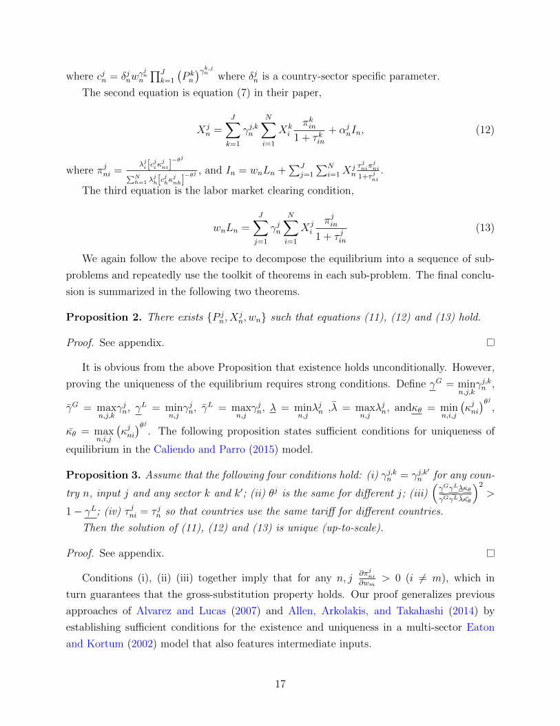
)γk,jn where δjn is a country-sector specific parameter.

The second equation is equation (7) in their paper,

Xjn =

J∑k=1

γj,kn

N∑i=1

Xki

πkin1 + τ kin

+ αjnIn, (12)

where πjni =λji [c

jiκjni]−θj

∑Nh=1 λ

jh[c

jhκjnh]−θj , and In = wnLn +

∑Jj=1

∑Ni=1X

jnτ jniπ

jni

1+τ jni.

The third equation is the labor market clearing condition,

wnLn =J∑j=1

γjn

N∑i=1

Xji

πjin1 + τ jin

(13)

We again follow the above recipe to decompose the equilibrium into a sequence of sub-

problems and repeatedly use the toolkit of theorems in each sub-problem. The final conclu-

sion is summarized in the following two theorems.

Proposition 2. There exists {P jn, X

jn, wn} such that equations (11), (12) and (13) hold.

Proof. See appendix.

It is obvious from the above Proposition that existence holds unconditionally. However,

proving the uniqueness of the equilibrium requires strong conditions. Define γG = minn,j,k

γj,kn ,

γG = maxn,j,k

γjn, γL = minn,j

γjn, γL = maxn,j

γjn, λ = minn,j

λjn ,λ = maxn,j

λjn, andκθ = minn,i,j

(κjni)θj

,

κθ = maxn,i,j

(κjni)θj

. The following proposition states sufficient conditions for uniqueness of

equilibrium in the Caliendo and Parro (2015) model.

Proposition 3. Assume that the following four conditions hold: (i) γj,kn = γj,k′

n for any coun-

try n, input j and any sector k and k′; (ii) θj is the same for different j; (iii)(γGγLλκθ

γGγLλκθ

)2

>

1− γL; (iv) τ jni = τ jn so that countries use the same tariff for different countries.

Then the solution of (11), (12) and (13) is unique (up-to-scale).

Proof. See appendix.

Conditions (i), (ii) (iii) together imply that for any n, j∂πjni∂wm

> 0 (i 6= m), which in

turn guarantees that the gross-substitution property holds. Our proof generalizes previous

approaches of Alvarez and Lucas (2007) and Allen, Arkolakis, and Takahashi (2014) by

establishing sufficient conditions for the existence and uniqueness in a multi-sector Eaton

and Kortum (2002) model that also features intermediate inputs.

17

5 Conclusion

TBD

References

Allen, T., and C. Arkolakis (2014): “Trade and the topography of the spatial economy,”

Quarterly Journal of Economics.

(2015): Elements of Advanced International Trade.

Allen, T., C. Arkolakis, and Y. Takahashi (2014): “Universal Gravity,” mimeo.

Alvarez, F., and R. E. Lucas (2007): “General Equilibrium Analysis of the Eaton-Kortum

Model of International Trade,” Journal of Monetary Economics, 54(6), 1726–1768.

Arkolakis, C. (2011): “A Unified Theory of Firm Selection and Growth,” NBER working paper,

17553.

Berman, A., and R. J. Plemmons (1979): “Nonnegative matrices,” The Mathematical Sciences,

Classics in Applied Mathematics,, 9.

Caliendo, L., and F. Parro (2015): “Estimates of the Trade and Welfare Effects of NAFTA,”

Review of Economic Studies, 82(1), 1–44.

Dekle, R., J. Eaton, and S. Kortum (2008): “Global Rebalancing with Gravity: Measuring

the Burden of Adjustment,” IMF Staff Papers, 55(3), 511–540.

Eaton, J., and S. Kortum (2002): “Technology, Geography and Trade,” Econometrica, 70(5),

1741–1779.

Gantmakher, F. R. (1959): The theory of matrices, vol. 131. American Mathematical Soc.

Ibe, O. C. (2011): Fundamentals of stochastic networks. John Wiley & Sons.

Karlin, S., and L. Nirenberg (1967): “On a theorem of P. Nowosad,” Journal of Mathematical

Analysis and Applications, 17(1), 61–67.

Mas-Colell, A., M. D. Whinston, and J. R. Green (1995): Microeconomic Theory. Oxford

University Press, Oxford, UK.

Melitz, M. J. (2003): “The Impact of Trade on Intra-Industry Reallocations and Aggregate

Industry Productivity,” Econometrica, 71(6), 1695–1725.

Meyer, C. D. (2000): Matrix analysis and applied linear algebra. Siam.

18

Stewart, G. W., and J.-g. Sun (1990): “Matrix perturbation theory,” .

19

6 Appendix A: proof for the theorem 1

The following is the whole proof of theorem 1.

Proof. Denote xk =

xk1

xk2

...

xkN

. Let ln yk = Aγ lnxk where yk =

yk1

yk2

...

ykN

. Thus, if the above

system 1 can be equivalently rewritten as

yki = λk

N∑j=1

Kkij

H∏h=1

(yhj)αkh k = 1, 2, .., H (14)

where αkh =(AβAγ

−1)kh

. Furthermore, the following equation is also equivalent with,

of the purpose of up to scale solution, the above equation system 14.

yki =

∑Nj=1 K

kij

∏Hh=1

(yhj)αkh∑N

n=1

∑Nm=1 K

kmn

∏Hh=1 (yhn)αkh

k = 1, 2, .., H. (15)

Thus, in the following we will focus on equation system 15 and 14.

Part (i)

In the following we are going to use Brouwer’s fixed-point theorem to prove the existence,

like Karlin and Nirenberg (1967) and Allen, Arkolakis, and Takahashi (2014).

First, construct the operators. Define operator T : RHN++ → RHN

++ where (T (y))i+N(k−1) =∑Nj=1K

kij

∏Hh=1(yhj )

αkh∑Nn=1

∑Nm=1K

kmn

∏Hh=1(yhn)

αkh . Obviously, T is a continuous operator.

Second, denoteMk = maxi,j

Kkij∑N

i=1Kkij

> 0, mk = mini,j

Kkij∑N

i=1Kkij

> 0. Thus, mk

∑Nm=1 K

kmj

∏Hh=1

(yhj)αkh ≤

Kk,ij

∏Hh=1

(yhj)αkh ≤ Mk

∑Nm=1K

kmj

∏Hh=1

(yhj)αkh , and mk ≤

∑Nj=1K

kij

∏Hh=1(yhj )

αkh∑Nn=1

∑Nm=1K

kmn

∏Hh=1(yhn)

αkh ≤

Mk. So define Y ={x|mk ≤ ykj ≤Mk, for all k, j

}. Obviously, for any y >> 0, T (y) ∈ Y .

Thus, there exists a solution in equation 15.

Part (ii)

In equation system, 14, suppose we have two different solutions in the sense of up to scale:{yh(0)j

},{yh(1)j

}which makes equations 14 hold and the corresponding eigenvalues are {λ0

k},

{λ1k}. Denote Mh = max

i

yh(1)i

yh(0)i

, mh = mini

yh(1)i

yh(0)i

. Notice that for at least one h, Mh

mh> 1. Thus,

equation system 14 can also be expressed as

20

yk(1)i

yk(0)i

=

λ1k

∑Nj=1K

kij

[∏Hh=1

(yh(1)j

yh(0)j

)αkh (yh(0)j

)αkh]yk(0)i

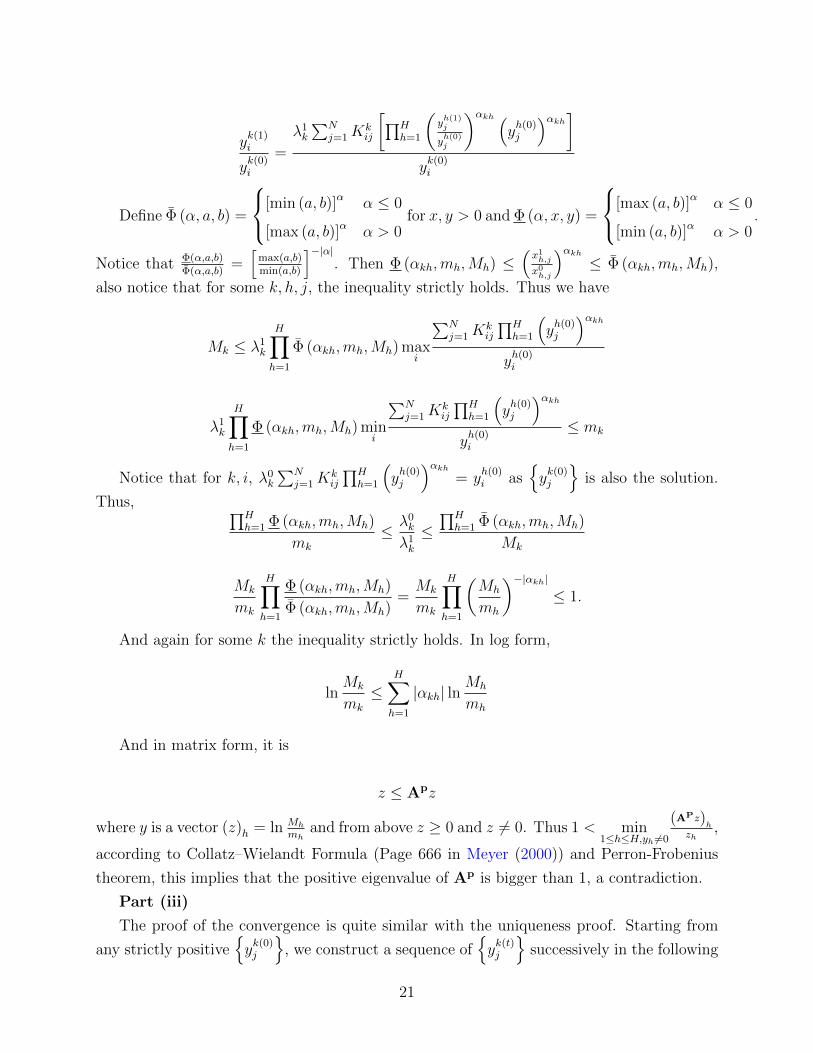
Define Φ (α, a, b) =

[min (a, b)]α α ≤ 0

[max (a, b)]α α > 0for x, y > 0 and Φ (α, x, y) =

[max (a, b)]α α ≤ 0

[min (a, b)]α α > 0.

Notice that Φ(α,a,b)

Φ(α,a,b)=[

max(a,b)min(a,b)

]−|α|. Then Φ (αkh,mh,Mh) ≤

(x1h,jx0h,j

)αkh≤ Φ (αkh,mh,Mh),

also notice that for some k, h, j, the inequality strictly holds. Thus we have

Mk ≤ λ1k

H∏h=1

Φ (αkh,mh,Mh) maxi

∑Nj=1K

kij

∏Hh=1

(yh(0)j

)αkhyh(0)i

λ1k

H∏h=1

Φ (αkh,mh,Mh) mini

∑Nj=1K

kij

∏Hh=1

(yh(0)j

)αkhyh(0)i

≤ mk

Notice that for k, i, λ0k

∑Nj=1K

kij

∏Hh=1

(yh(0)j

)αkh= y

h(0)i as

{yk(0)j

}is also the solution.

Thus, ∏Hh=1 Φ (αkh,mh,Mh)

mk

≤ λ0k

λ1k

≤∏H

h=1 Φ (αkh,mh,Mh)

Mk

Mk

mk

H∏h=1

Φ (αkh,mh,Mh)

Φ (αkh,mh,Mh)=Mk

mk

H∏h=1

(Mh

mh

)−|αkh|≤ 1.

And again for some k the inequality strictly holds. In log form,

lnMk

mk

≤H∑h=1

|αkh| lnMh

mh

And in matrix form, it is

z ≤ Apz

where y is a vector (z)h = ln Mh

mhand from above z ≥ 0 and z 6= 0. Thus 1 < min

1≤h≤H,yh 6=0

(APz)h

zh,

according to Collatz–Wielandt Formula (Page 666 in Meyer (2000)) and Perron-Frobenius

theorem, this implies that the positive eigenvalue of Ap is bigger than 1, a contradiction.

Part (iii)

The proof of the convergence is quite similar with the uniqueness proof. Starting from

any strictly positive{yk(0)j

}, we construct a sequence of

{yk(t)j

}successively in the following

21

way,

yk(t)i = λtk

N∑j=1

Kkij

H∏h=1

(yh(t−1)j

)αkh.

where λtk =∑N

i=1

∑Nj=1K

kij

∏Hh=1

(yh(t−1)j

)αkh. It can be rewritten as

yk(t)i

yk(t−1)i

=

λtk∑N

j=1Kkij

[∏Hh=1

(yh(t−1)j

yh(t−2)j

)αkh (yh(t−2)j

)αkh]yk(t−1)i

.

Also we have Φ (αkh,mth,M

th) ≤

(yk(t)j

yk(t−1)j

)αkh≤ Φ (αkh,m

th,M

th) where M t

h = maxi

yk(t)i

yk(t−1)i

,

mth = min

i

yk(t)i

yk(t−1)i

and Φ (α, x, y), Φ (α, x, y) are the same in the proof of uniqueness. Thus,

we have

M tk 6 λtk

H∏h=1

Φ(αkh,m

t−1h ,M t−1

h

)maxi

∑Nj=1 K

kij

∏Hh=1

(yh(t−2)j

)αkhyk(t−1)i

λtk

H∏h=1

Φ(αkh,m

t−1h ,M t−1

h

)mini

∑Nj=1K

kij

∏Hh=1

(yh(t−2)j

)αkhyk(t−1)i

6 mtk

Cancel out yk(t−1)i = λt−1

k

∑Nj=1K

kij

∏Hh=1

(yh(t−2)j

)αkhand put the two inequalities to-

gether, ∏Hh=1 Φ

(αkh,m

t−1h ,M t−1

h

)mtk

6λt−1k

λtk6

∏Hh=1 Φ

(αkh,m

t−1h ,M t−1

h

)M t

k

.

Thus,

M tk

mtk

H∏h=1

Φ(αkh,m

t−1h ,M t−1

h

)Φ(αkh,m

t−1h ,M t−1

h

) =M t

k

mtk

H∏h=1

(M t−1

h

mt−1h

)−|αkh|6 1

In log form,

lnM t

k

mtk

6H∑h=1

|αkh| lnM t−1

h

mt−1h

.

And in matrix form, it is

22

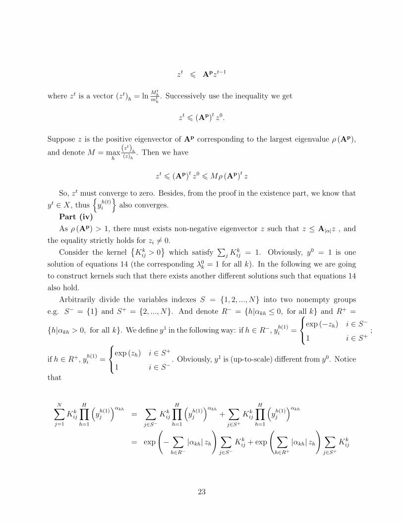
zt 6 Apzt−1

where zt is a vector (zt)h = lnMth

mth. Successively use the inequality we get

zt 6 (Ap)t z0.

Suppose z is the positive eigenvector of Ap corresponding to the largest eigenvalue ρ (Ap),

and denote M = maxh

(zt)h

(z)h. Then we have

zt 6 (Ap)t z0 6Mρ (Ap)t z

So, zt must converge to zero. Besides, from the proof in the existence part, we know that

yt ∈ X, thus{yh(t)i

}also converges.

Part (iv)

As ρ (Ap) > 1, there must exists non-negative eigenvector z such that z ≤ A|α|z , and

the equality strictly holds for zi 6= 0.

Consider the kernel{Kkij > 0

}which satisfy

∑jK

kij = 1. Obviously, y0 = 1 is one

solution of equations 14 (the corresponding λ0k = 1 for all k). In the following we are going

to construct kernels such that there exists another different solutions such that equations 14

also hold.

Arbitrarily divide the variables indexes S = {1, 2, ..., N} into two nonempty groups

e.g. S− = {1} and S+ = {2, ..., N}. And denote R− = {h|αkh ≤ 0, for all k} and R+ =

{h|αkh > 0, for all k}. We define y1 in the following way: if h ∈ R−, yh(1)i =

exp (−zh) i ∈ S−

1 i ∈ S+;

if h ∈ R+, yh(1)i =

exp (zh) i ∈ S+

1 i ∈ S−. Obviously, y1 is (up-to-scale) different from y0. Notice

that

N∑j=1

Kkij

H∏h=1

(yh(1)j

)αkh=

∑j∈S−

Kkij

H∏h=1

(yh(1)j

)αkh+∑j∈S+

Kkij

H∏h=1

(yh(1)j

)αkh= exp

(−∑h∈R−

|αkh| zh

) ∑j∈S−

Kkij + exp

(∑h∈R+

|αkh| zh

)∑j∈S+

Kkij

23

If k ∈ R−,N∑j=1

Kkij

H∏h=1

(yh(1)j

)αkh= exp

(∑h∈R+

|αkh| zh

)yk(1)i

where yk(1)i = exp

(−∑H

h=1 |αkh| zh)∑

j∈S− Kkij+∑

j∈S+ Kkij.Notice exp

(−∑H

h=1 |αkh| zh)≤

yk(1)i ≤ 1. Also recall from the above that zk ≤

∑Hh=1 |αkh| zh, thus (from the above

definition of yk(1)i ) exp

(−∑H

h=1 |αkh| zh)≤ y

k(1)i ≤ 1. By adjusting the value of Kk

ij

while keeping∑

jKk,ij = 1, we can always make yk(1)i = y

k(1)i . At the same time, set

λ1k = exp

(−∑

h∈R+ |αkh| zh), equations set Ξk holds.

If k ∈ R+, similarly, we can again show that Ξk holds. Thus, there exists multiple

equilibria.

7 Appendix B: Proof of Lemma 2

Proof. If∑

j tij < sii, write A = S (I− S−1T).

Notice that S−1 is also a diagonal matrix and its diagonal element is 1sii

. Thus A−1 exists

if and only if (I− S−1T)−1

exists, and A−1 = (I− S−1T)−1

S−1. As S−1T is a non-negative

matrix, according to Lemma 2.1 in Chapter 6 of Berman and Plemmons (1979), (I− S−1T)−1

exists if and only if the spectral radius of S−1T is smaller than 1, i.e. ρ (S−1T) < 1. Denote

S−1T = Q = (qij) where qij =tijsii≥ 0, thus

∑j

qij =∑j tij

sii< 1

Let us construct an auxiliary matrix Q = (qik) where qik = qik for all k 6= n (n is

the dimension of the square matrices) qin = 1 −∑k 6=n

qik. Thus∑

k qik = 1. Notice that(Q)T∗ 1 = 1 ∗ 1 i.e. unit vector is the positive eigenvector and 1 is the positive eigenvalue.

According to Perron-Frobenius theorem ρ(Q)

= 1. Also notice that Q > Q, at the same

time the eigenvalue must increase with the element matrix ( dλdqik

> 0, according to corollary

2.4 on page 185 of Stewart and Sun (1990)). Thus ρ (S−1T) < 1. So (I− S−1T)−1

=[

k=

0]∞∑

(S−1T)k ≥ 0, thus A−1 = (I− S−1T)

−1S−1 ≥ 0. Furthermore, if T > 0, A−1 > 0.

If∑

j tji < sii, write A = (I−TS−1) S. The rest is similar with the above.

24

8 Appendix C: Proofs of propositions in various trade

models

Before moving into the examples, we introduce some notation. To use the existence and

uniqueness theorems in the last section, we need to know the monotonicity relationship

between variables and equations in the equilibrium system. Since in complex equilibrium

systems there are too many variables and equations, to make things simpler, we will use the

differential notation dx, dy rather than derivative notation ∂y∂x

. For example, in equation

f (x, y) = 0, we will differentiate it as f1 (x, y) dx + f2 (x, y) dy = 0. To know the derivative

∂yi∂xj

we just need to set dxk =

0 k 6= j

1 k = jand solve dyi which will be ∂yi

∂xj. This notation also

gives us the flexibility to transform the variables, e.g. in order to know the elasticity ∂lnyi∂lnxj

,

we just need to set dxkxk

=

0 k 6= j

1 k = jand solve dyi

yiwhich will be ∂lnyi

∂lnxj. As we will see (in

the appendix), this makes things easier.

8.1 Proof Heterogeneous firms with arbitrary country-specific pro-

ductivity distributions

The following is the proof of Proposition 1 which establish the existence and uniqueness of

Melitz model with fixed entry and non-standard firm distribution.

Proof. To facilitate the proof, we first define some notations.

Denote the excess expenditure Eej =

∑k ykj − yjLj, excess wage Ew

i = σ−1σ

∑j yij +∑

j wifij´∞z∗ijmi(z)dz − wiLi, and excess income EI

i =∑

j yij − yiLi. Differentiate Eej , E

wi

and EIi ,

dEej =

∑k

ykjdwkwk−∑k

Mkj

dz∗kjz∗kj− yjLj

dyjyj

(16)

dEwi = Ew

i

dwiwi−∑j

M1ij

dz∗ijz∗ij

(17)

dEIi = −

∑j

Mij

dz∗ijz∗ij

+∑j

yijdwiwi− yiLi

dyiyi

(18)

25

where for convenience we define4Nkj = wkfkjmk(z∗kj)z

∗ij, Mij = (σ − 1) yij + σ4Nij , and

M1ij = (σ−1)2

σyij + σ4Nij. Besides, differentiate equation 7,

dz∗ijz∗ij

= −dPjPj

+σ

σ − 1

dwiwi

+1

1− σdyjyj. (19)

Step 1: prove the existence and uniqueness of {Pi} in equation 8 with {wi, yi}taken as given.

The proof of both uniqueness and existence is done by showing that excess expenditure,

Eej , is monotonic on Pj and the range is (0,∞).

First, given wage and income, there always exists a price index that satisfy (8). Notice

that according to equation (7), for any given Pi, wi and yi there will always exist a cutoff

z∗ij. And also given any w and y, when Pj → 0, z∗kj →∞, so

Eej =

∑k

σwkfkj

ˆ ∞z∗kj

(z

z∗kj

)σ−1

mk(z)dz − yjLj → −yjLj

and if Pj → ∞, z∗kj → 0, condition 1 implies that Eej → ∞. Besides, obviously Ee

j is

continuous with respect to Pj. According to the intermediate value theorem, there must

exist a price Pj satisfying (8).

Second, the solution of price index is unique in each market. Given the wage and expen-

diture, after inserting the expression of cutoff z∗kj into the excess expenditure Eej , the only

unknown variable is the price index is Pj, to prove the uniqueness of the price index we need

only to prove Eej is monotonic with respect to (w.r.t.) Pj. Wage and expenditure are given

means that dwiwi

=dyjyj

= 0 for all i and j. Insert equation (19) into equation (16), we get

dEej =

∑k

ykjdwkwk−∑k

Mkj

dz∗kjz∗kj− yjLj

dyjyj

=∑k

MkjdPjPj

As Mkj is positive, thus Eej is increasing with Pj.

All in all, there exists a unique price given wage and income solving equation (8).

Step 2: prove the existence and uniqueness of {wi} in equation (9) with {yi}taken as given and {Pi} endogenously solved in last step.

Existence part of step 2:

In this step, to simplify notations, define a few functions: Zij (wi, Pj, y) = cij(wi)

1+ 1σ−1

Pjy1

σ−1j

,

where Zij (wi, Pj, y) increases w.r.t wi and decreases w.r.t. Pj; Fi (z∗) = (σ − 1)

´∞z∗

(zz∗

)σ−1mi(z)dz+´∞

z∗mi(z)dz, Fi (z) decreases w.r.t z∗, moreover if z∗ → 0, Fi (z

∗) > (σ − 1)Gi(z∗) → ∞; if

26

z∗ → ∞, Fi (z∗) < (σ − 1 + 1)Gi(z

∗) → 0 ; Pj (w, yj) is the implicit function of price from

equation (8) according to step 1. Here insert equation (19) into equation (16), notice here

as equation (8) holds, thus dEej = 0. Thus we have

dPjPj

=

∑k σ[

(σ−1)2

σykj + σ4Nkj

]dwkwk− σ

∑k4Nkj

dyjyj∑

k [(σ − 1) ykj + σ4Nkj]

=

∑k σM

1kjdwkwk− σ

∑k4Nkj

dyjyj∑

kMkj

(20)

which means that Pj (w, yj) increases with w and decreases with yj.

Notice that equation (9) is equivalent with Li =∑

j fijFi (Zij (wi, Pj (w, yj) , y)).

Now we proceed by verifying the conditions of Lemma 1. Notice that the above equation

can be written as Gi (w′, wi) =

∑j fijFi (Zij (wi, Pj (w′, yj) , y))− Li = 0.

Condition (i): If wi → 0 ,Zij (wi, Pj (w′, yj) , y)→ 0 thus∑

j fijFi (Zij (wi, Pj (w′, yj) , y))→∞ ; wi → ∞ ,Zij (wi, Pj (w′, yj) , y) → ∞,

∑j fijFi (Zij (wi, Pj (w′, yj) , y)) → 0. According

to the intermediate value theorem, there exists wi such that Gi (w′, wi) = 0.

Condition (ii): As Zij (wi, Pj, y) is increasing w.r.t wi and Fi (z) is decreasing w.r.t z∗,∑j fijFi (Zij (wi, Pj (w′, yj) , y)) decreases w.r.t wi i.e. ∂Gi(w

′,wi)∂wi

< 0; Besides, Zij (wi, Pj, y)

decreases w.r.t Pj and Pj (w′, yj) increases w.r.t w′, thus∑

j fijFi (Zij (wi, Pj (w′, y) , y)) in-

creases w.r.t w′ i.e. ∂Gi(w′,wi)

∂w′j> 0. ∂Gi(w

′,wi)∂wi

∂Gi(w′,wi)

∂w′j< 0, condition (ii) is also satisfied.

Condition (iii):

We will first see how the price index change if the wage w0 becomes tw0(t 6= 1).

If t increase, to keep equation (8) yjLj =∑

k σtwkfkj´∞z∗kj

(zz∗kj

)σ−1

mk(z)dz hold, z∗kj =

ckj(tw0

k)1+ 1

σ−1

(Pj(tw0,yj))jy1

σ−1j

has to increase. Moreover, if t → 0, z∗kj → 0; if t → ∞, z∗kj → ∞.

Thus ∇p (t) =P(tw0,y)tσP (w0,y)

is an decreasing vector function w.r.t t, ∇p (1) = 1, and if t → 0,

∇p (t)→∞; if t→∞, ∇p (t)→ 0.

Denote vector ∇w (t) =(wtw0

)1+ 1σ−1 where wi is defined in Gi (tw

0, wi) = 0. Then

Zij (wi, Pj, y) =(∇w(t))i(∇p(t))j

z0ijwhere z0

ij = Zij (w0, Pj (w0, yj) , y) . Obviously,(∇w(t))i

maxj

(∇p(t))j≤

(∇w(t))i(∇p(t))j

≤ (∇w(t))iminj

(∇p(t))j. Thus

∑j

fijFi

(∇w (t))iminj

(∇p (t))jz0ij

≤ Li =∑j

fijFi

((∇w (t))i(∇p (t))j

z0ij

)≤∑j

fijFi

(∇w (t))imaxj

(∇p (t))jz0ij

.

27

Also notice that there exists a constant si satisfying Li =∑

j fijFi(siz

0ij

). Thus

∑j

fijFi

((∇w (t))imin∇p (t)

z0ij

)≤∑j

fijFi(siz

0ij

)≤∑j

fijFi

((∇w (t))i

max∇p (t)z0ij

)

which means that(∇w(t))i

maxj

(∇p(t))j≤ si ≤ (∇w(t))i

minj

(∇p(t))ji.e.

siminj

(∇p (t))j ≤ (∇w (t))i ≤ simaxj

(∇p (t))j

As the range of ∇p (t) is (0,∞), so is (∇w (t))i, specifically, if t → 0, (∇w (t))i → ∞i.e. t

wi→ 0; if t → ∞, (∇w (t))i → 0 i.e. t

wi→ ∞. Condition (iii) also holds. Thus existence

is proven.

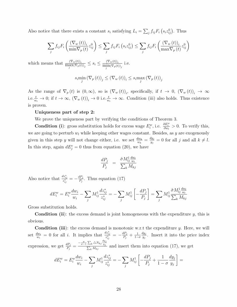
Uniqueness part of step 2:

We prove the uniqueness part by verifying the conditions of Theorem 3.

Condition (i): gross substitution holds for excess wage Ewi , i.e.

∂Ewi∂wl

> 0. To verify this,

we are going to perturb wl while keeping other wages constant. Besides, as y are exogenously

given in this step y will not change either, i.e. we set dwkwk

=dyjyj

= 0 for all j and all k 6= l.

In this step, again dEej = 0 thus from equation (20), we have

dPjPj

=σM1

ljdwlwl∑

kMkj

Also notice thatdz∗ijz∗ij

= −dPjPj

. Thus equation (17)

dEwi = Ew

i

dwiwi−∑j

M1ij

dz∗ijz∗ij

= −∑j

M1ij

[−dPjPj

]=∑j

M1ij

σM1ljdwlwl∑

kMkj

Gross substitution holds.

Condition (ii): the excess demand is joint homogeneous with the expenditure y, this is

obvious.

Condition (iii): the excess demand is monotonic w.r.t the expenditure y. Here, we will

set dwiwi

= 0 for all i. It implies thatdz∗ijz∗ij

= −dPjPj

+ 11−σ

dyjyj

. Insert it into the price index

expression, we getdPjPj

=− σσ−1

∑k4Nkj

dyjyj∑

kMkjand insert them into equation (17), we get

dEwi = Ew

i

dwiwi−∑j

M1ij

dz∗ijz∗ij

= −∑j

M1ij

[−dPjPj

+1

1− σdyjyj

]=

28

= −∑j

M1ij

[− σσ−1

∑k4Nkj∑

kMkj

+1

1− σ

]dyjyj

=∑j

M1ij

yjLj∑kMkj

dyjyj

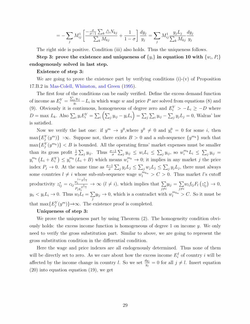
The right side is positive. Condition (iii) also holds. Thus the uniqueness follows.

Step 3: prove the existence and uniqueness of {yi} in equation 10 with {wi, Pi}endogenously solved in last step.

Existence of step 3:

We are going to prove the existence part by verifying conditions (i)-(v) of Proposition

17.B.2 in Mas-Colell, Whinston, and Green (1995).

The first four of the conditions can be easily verified. Define the excess demand function

of income as EYi =

∑j yij

yi−Li in which wage w and price P are solved from equations (8) and

(9). Obviously it is continuous, homogeneous of degree zero and EYi > −Li ≥ −D where

D = max Lk. Also∑

i yiEYi =

∑i

(∑j yij − yiLi

)=∑

j

∑i yij −

∑j yjLj = 0, Walras’ law

is satisfied.

Now we verify the last one: if ym → y0,where y0 6= 0 and y0i = 0 for some i, then

max{EYj (ym)}�∞. Suppose not, there exists B > 0 and a sub-sequence {ymk} such that

max{EYj (ymk)} < B is bounded. All the operating firms’ market expenses must be smaller

than its gross profit 1σ

∑j yij. Thus σ−1

σ

∑j yij ≤ wiLi ≤

∑j yij, so wmki Li ≤

∑j yij =

ymki(Li + EY

i

)≤ ymki (Li +B) which means wmki → 0; it implies in any market j the price

index Pj → 0. At the same time as σ−1σ

∑j yjLj ≤

∑j wjLj ≤

∑j yjLj, there must always

some countries l 6= i whose sub-sub-sequence wage wmknl > C > 0. Thus market l’s cutoff

productivity z∗lj = cljw

1+ 1σ−1

l

Pjy1

σ−1j

→ ∞ (l 6= i), which implies that∑j 6=iylj =

∑j 6=iwlfljFl

(z∗lj)→ 0,

yli < yiLi → 0. Thus wlLl =∑j

ylj → 0, which is a contradict with wmknl > C. So it must be

that max{EYj (ym)}�∞. The existence proof is completed.

Uniqueness of step 3:

We prove the uniqueness part by using Theorem (2). The homogeneity condition obvi-

ously holds: the excess income function is homogeneous of degree 1 on income y. We only

need to verify the gross substitution part. Similar to above, we are going to represent the

gross substitution condition in the differential condition.

Here the wage and price indexes are all endogenously determined. Thus none of them

will be directly set to zero. As we care about how the excess income EIi of country i will be

affected by the income change in country l. So we setdyjyj

= 0 for all j 6= l. Insert equation

(20) into equation equation (19), we get

29

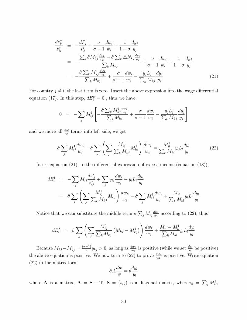
dz∗ijz∗ij

= −dPjPj

+σ

σ − 1

dwiwi

+1

1− σdyjyj

= −∑

k σM1kjdwkwk− σ

∑k4Nkj

dyjyj∑

kMkj

+σ

σ − 1

dwiwi

+1

1− σdyjyj

= −σ∑

kM1kjdwkwk∑

kMkj

+σ

σ − 1

dwiwi− yjLj∑

kMkj

dyjyj

(21)

For country j 6= l, the last term is zero. Insert the above expression into the wage differential

equation (17). In this step, dEwi = 0 , thus we have.

0 = −∑j

M1ij

[−σ∑

kM1kjdwkwk∑

kMkj

+σ

σ − 1

dwiwi− yjLj∑

kMkj

dyjyj

]

and we move all dww

terms into left side, we get

σ∑j

M1ij

dwiwi− σ

∑k

(∑j

M1ij∑

kMkj

M1kj

)dwkwk

=M1

il∑kMkl

ylLldylyl

(22)

Insert equation (21), to the differential expression of excess income (equation (18)),

dEIi = −

∑j

Mij

dz∗ijz∗ij

+∑j

yijdwiwi− yiLi

dyiyi

= σ∑k

(∑j

M1ij∑

kMkj

Mkj

)dwkwk− σ

∑j

M1ij

dwiwi

+Mil∑kMkl

ylLldylyl

Notice that we can substitute the middle term σ∑

jM1ijdwiwi

according to (22), thus

dEIi = σ

∑k

(∑j

M1ij∑

kMkj

(Mkj −M1

kj

)) dwkwk

+Mil −M1

il∑kMkl

ylLldylyl

Because Mkj−M1kj = (σ−1)

σykj > 0, as long as dwk

wkis positive (while we set dyl

ylbe positive)

the above equation is positive. We now turn to (22) to prove dwkwk

is positive. Write equation

(22) in the matrix form

σAdw

w= b

dylyl

where A is a matrix, A = S − T, S = (sik) is a diagonal matrix, wheresii =∑

jM1ij,

30

and T = (tik), tik =∑

j

M1ij∑

kMkjM1

kj. Notice that the row summation of T∑

k tik =∑k

∑j

M1ij∑

kMkjM1

kj =∑

jM1ij

∑kM

1kj∑

kMkj<∑

jM1ij = sii. Then according to Lemma 2, we

know that A is invertible and A−1 >> 0. As a result dwkwk

is positive (while we set dylyl

be

positive). Uniqueness is proven.

The above three steps together is the complete proof of Proposition 1.

8.2 Proof for Multi-sector trade model with input-output linkages

We first give the proof of Proposition 2.

Proof. Step 1: prove the existence and uniqueness of price P in equation 11 with

wn, goods expenditure Xjn, and resident expenditure In.

Proof can be seen in above examples 3 and 6.

Step 2: prove the existence and uniqueness of production Xjn in equation (12)

with wn exogenously given and P endogenously solved in equation (11).

Substitute the expression of In into (24), we obtain

Xjn =

J∑k=1

N∑i=1

γj,knπkin

1 + τ kinXki + αjn

J∑k=1

N∑m=1

τ knmπknm

1 + τ knmXkn + αjnwnLn (23)

Notice that given price if we write the above equations in the form of matrix it becomes

X = AX + b

where X =

X1

1

...

XJ1

...

XJN

is a NJ dimension vector; A =(a(n−1)J+j,(i−1)J+k

)is a NJ-by-NJ ma-

trix whose element is a(n−1)J+j,(i−1)J+k = γj,knπkin

1+τkin+a(n−1)J+j,(i−1)J+k where a(n−1)J+j,(i−1)J+k =αjn

∑Nm=1 τ

knm

πknm1+τknm

n = i

0 n 6= i; b =

(b(n−1)J+j

)is also a NJ dimension vector in which

b(n−1)J+j = αjnwnLn. The above matrix equation can be written as (I−A)X = b. No-

31

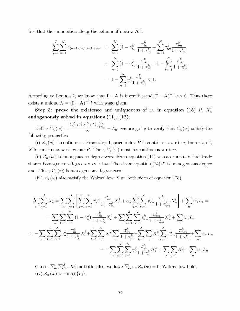
tice that the summation along the column of matrix A is

J∑j=1

N∑n=1

a(n−1)J+j,(i−1)J+k =N∑n=1

(1− γkn

) πkin1 + τ kin

+N∑m=1

τ kimπkim

1 + τ kim

=N∑n=1

(1− γkn

) πkin1 + τ kin

+ 1−N∑m=1

πkim1 + τ kim

= 1−N∑n=1

γknπkin

1 + τ kin< 1.

According to Lemma 2, we know that I −A is invertible and (I−A)−1 >> 0. Thus there

exists a unique X = (I−A)−1 b with wage given.

Step 3: prove the existence and uniqueness of wn in equation (13) P , Xjn

endogenously solved in equations (11), (12).

Define Zn (w) =

∑Jj=1 γ

jn∑Ni=1X

ji

πjin

1+τjin

wn− Ln. we are going to verify that Zn (w) satisfy the

following properties.

(i) Zn (w) is continuous. From step 1, price index P is continuous w.r.t w; from step 2,

X is continuous w.r.t w and P . Thus, Zn (w) must be continuous w.r.t w.

(ii) Zn (w) is homogeneous degree zero. From equation (11) we can conclude that trade

shareπ homogeneous degree zero w.r.t w. Then from equation (24) X is homogeneous degree

one. Thus, Zn (w) is homogeneous degree zero.

(iii) Zn (w) also satisfy the Walras’ law. Sum both sides of equation (23)

∑n

J∑j=1

Xjn =

∑n

J∑j=1

[J∑k=1

N∑i=1

γj,knπkin

1 + τ kinXki + αjn

J∑k=1

N∑m=1

τ knmπknm

1 + τ knmXkn

]+∑n

wnLn =

=∑n

J∑k=1

N∑i=1

(1− γkn

) πkin1 + τ kin

Xki +

∑n

J∑k=1

N∑m=1

τ knmπknm

1 + τ knmXkn +

∑n

wnLn

= −∑n

J∑k=1

N∑i=1

γknπkin

1 + τ kinXki +

J∑k=1

N∑i=1

Xki

∑n

πkin1 + τ kin

+J∑k=1

∑n

Xkn

N∑m=1

τ knmπknm

1 + τ knm+∑n

wnLn

= −∑n

J∑k=1

N∑i=1

γknπkin

1 + τ kinXki +

∑n

J∑j=1

Xjn +

∑n

wnLn

Cancel∑

n

∑Jj=1X

jn on both sides, we have

∑nwnZn (w) = 0, Walras’ law hold.

(iv) Zn (w) > −maxi{Li}.

32

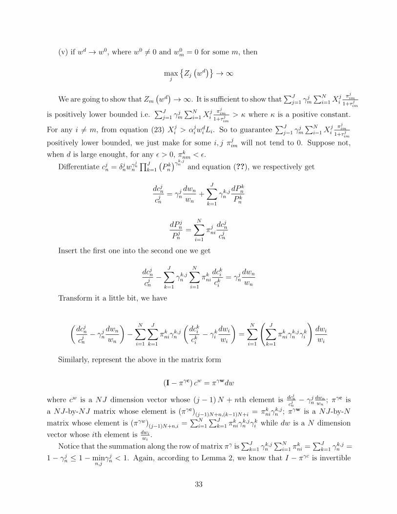
(v) if wd → w0, where w0 6= 0 and w0m = 0 for some m, then

maxj

{Zj(wd)}→∞

We are going to show that Zm(wd)→∞. It is sufficient to show that

∑Jj=1 γ

jm

∑Ni=1X

ji

πjim1+τ jim

is positively lower bounded i.e.∑J

j=1 γjm

∑Ni=1X

ji

πjim1+τ jim

> κ where κ is a positive constant.

For any i 6= m, from equation (23) Xji > αjiw

diLi. So to guarantee

∑Jj=1 γ

jm

∑Ni=1X

ji

πjim1+τ jim

positively lower bounded, we just make for some i, j πjim will not tend to 0. Suppose not,

when d is large enought, for any ε > 0, πknm < ε.

Differentiate cjn = δjnwγjnn

∏Jk=1

(P kn

)γk,jn and equation (??), we respectively get

dcjncjn

= γjndwnwn

+J∑k=1

γk,jndP k

n

P kn

dP jn

P jn

=N∑i=1

πjnidcjncjn

Insert the first one into the second one we get

dcjncjn−

J∑k=1

γk,jn

N∑i=1

πknidckicki

= γjndwnwn

Transform it a little bit, we have

(dcjncjn− γjn

dwnwn

)−

N∑i=1

J∑k=1

πkniγk,jn

(dckicki− γki

dwiwi

)=

N∑i=1

(J∑k=1

πkniγk,jn γki

)dwiwi

Similarly, represent the above in the matrix form

(I− πγc) cw = πγwdw

where cw is a NJ dimension vector whose (j − 1)N + nth element is dcjncjn− γjn

dwnwn

; πγc is

a NJ-by-NJ matrix whose element is (πγc)(j−1)N+n,(k−1)N+i = πkniγk,jn ; πγw is a NJ-by-N

matrix whose element is (πγw)(j−1)N+n,i =∑N

i=1

∑Jk=1 π

kniγ

k,jn γki while dw is a N dimension

vector whose ith element is dwiwi

.

Notice that the summation along the row of matrix πγ is∑J

k=1 γk,jn

∑Ni=1 π

kni =

∑Jk=1 γ

k,jn =

1 − γjn ≤ 1 −minn,j

γjn < 1. Again, according to Lemma 2, we know that I − πγc is invertible

33

and (I − πγc)−1 >> 0. Also one can verify that the summation of each row of (πγc)t is

smaller than

(1−min

n,jγjn

)t, thus the summation of each row (I − πγc)−1 is smaller than

1

minn,j

γjn. (I − πγc)−1 is upper bounded.

As ws → w0, if i 6= m, wi > 0, so we don’t have to care about the value ofdcktckt− γkt dwtwt

w.r.t dwiwi

(as dwiwi

will almost be zero) but only focus on the value w.r.t dwmwm

. Thus the

(πγww)(j−1)N+n,i becomes∑J

k=1 πknmγ

k,jn γkm

dwmwm

.

According to the above, πknm < ε, thus (πγww)(j−1)N+n,i < ε∑J

k=1 γk,jn γkm

dwmwm

. Thus

0 <dcktckt−γkt dwtwt

< εC where C is a constant. Notice that for t 6= mdcktckt→ 0 for dckm

ckm→ γkm

dwmwm

.

Besides, notice that

dπknmπknm

= θk(dP k

n

P kn

− dckmckm

)= −θk

(dckmckm−

N∑i=1

πknidcknckn

)

It means that when the share is small enough, it will increase w.r.t wm, so it can’t be

that πknm → 0. A contradiction.

Uniqueness:

We now give the proof of Proposition 3.

We are going to prove the uniqueness under the conditions: i) γj,k1n = γj,k2n for any n, j

and any k1 and k2; ii) θj is the same for different j; iii)(γGγLλκθ

γGγLλκθ

)2

> 1 − γL; iv) τ jni = τ jn

countries use the same tariff for different countries.

Proof. For the convenience of proving the uniqueness, we use the following two equations

(24) and (25) instead to replace equations (12) and (13).

Y jn =

N∑i=1

(J∑k=1

γj,ki Y ki + αji Ii

)πjin

1 + τ jin(24)

where πjni =λji [c

jiκjni]−θj

∑Nh=1 λ

jh[c

jhκjnh]−θj , and In = wnLn +

∑Jj=1

∑Ni=1

τ jni1+τ jni

πjni

(∑Jk=1 γ

j,kn Y k

n + αjnIn

),

under same tariff In = αn

(wnLn +

∑Jj=1

∑Ni=1

τ jni1+τ jni

πjni∑J

k=1 γj,kn Y k

n

)where αn = 1∑J

j=1

∑Ni=1

αjnπjni

1+τjni

.

This equation is about production balance. The dimension of this equation is also J ×N .

34

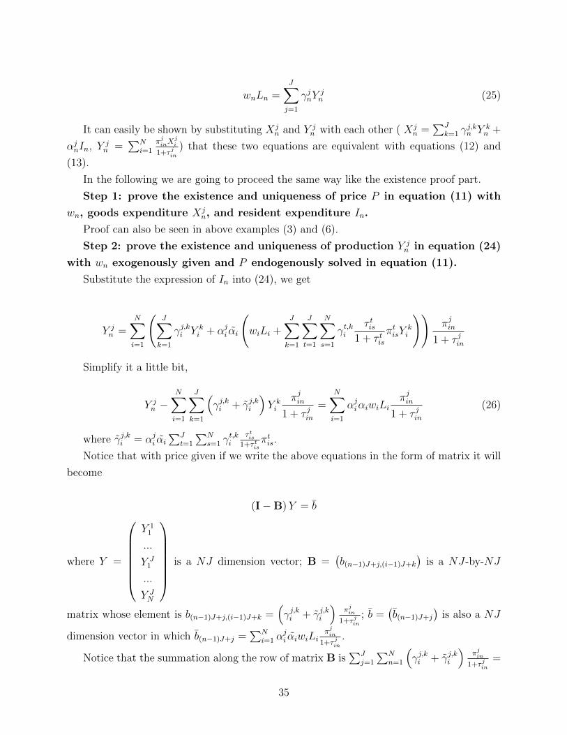
wnLn =J∑j=1

γjnYjn (25)

It can easily be shown by substituting Xjn and Y j

n with each other ( Xjn =

∑Jk=1 γ

j,kn Y k

n +

αjnIn, Y jn =

∑Ni=1

πjinXji

1+τ jin) that these two equations are equivalent with equations (12) and

(13).

In the following we are going to proceed the same way like the existence proof part.

Step 1: prove the existence and uniqueness of price P in equation (11) with

wn, goods expenditure Xjn, and resident expenditure In.

Proof can also be seen in above examples (3) and (6).

Step 2: prove the existence and uniqueness of production Y jn in equation (24)

with wn exogenously given and P endogenously solved in equation (11).

Substitute the expression of In into (24), we get

Y jn =

N∑i=1

(J∑k=1

γj,ki Y ki + αji αi

(wiLi +

J∑k=1

J∑t=1

N∑s=1

γt,kiτ tis

1 + τ tisπtisY

ki

))πjin

1 + τ jin

Simplify it a little bit,

Y jn −

N∑i=1

J∑k=1

(γj,ki + γj,ki

)Y ki

πjin1 + τ jin

=N∑i=1

αjiαiwiLiπjin

1 + τ jin(26)

where γj,ki = αji αi∑J

t=1

∑Ns=1 γ

t,ki

τ tis1+τ tis

πtis.

Notice that with price given if we write the above equations in the form of matrix it will

become

(I−B)Y = b

where Y =

Y 1

1

...

Y J1

...

Y JN

is a NJ dimension vector; B =(b(n−1)J+j,(i−1)J+k

)is a NJ-by-NJ

matrix whose element is b(n−1)J+j,(i−1)J+k =(γj,ki + γj,ki

)πjin

1+τ jin; b =

(b(n−1)J+j

)is also a NJ

dimension vector in which b(n−1)J+j =∑N

i=1 αji αiwiLi

πjin1+τ jin

.

Notice that the summation along the row of matrix B is∑J

j=1

∑Nn=1

(γj,ki + γj,ki

)πjin

1+τ jin=

35

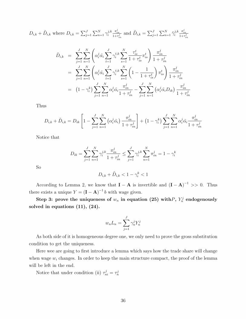
Di,k + Di,k where Di,k =∑J

j=1

∑Nn=1 γ

j,ki

πjin1+τ jin

and Di,k =∑J

j=1

∑Nn=1 γ

j,ki

πjin1+τ jin

Di,k =J∑j=1

N∑n=1

(αji αi

J∑t=1

γt,ki

N∑s=1

τ tis1 + τ tis

πtis

)πjin

1 + τ jin

=J∑j=1

N∑n=1

(αji αi

J∑t=1

γt,ki

N∑s=1

(1− 1

1 + τ tis

)πtis

)πjin

1 + τ jin

=(1− γki

) J∑j=1

N∑n=1

αji αiπjin

1 + τ jin−

J∑j=1

N∑n=1

(αji αiDik

) πjin1 + τ jin

Thus

Di,k + Di,k = Dik

[1−

J∑j=1

N∑n=1

(αji αi

) πjin1 + τ jin

]+(1− γki

) J∑j=1

N∑n=1

αji αiπjin

1 + τ jin

Notice that

Dik =J∑j=1

N∑n=1

γj,kiπjin

1 + τ jin≤

J∑j=1

γj,ki

N∑n=1

πjin = 1− γki

So

Di,k + Di,k < 1− γki < 1

According to Lemma 2, we know that I − A is invertible and (I−A)−1 >> 0. Thus

there exists a unique Y = (I−A)−1 b with wage given.

Step 3: prove the uniqueness of wn in equation (25) withP , Y jn endogenously

solved in equations (11), (24).

wnLn =J∑j=1

γjnYjn

As both side of it is homogeneous degree one, we only need to prove the gross substitution

condition to get the uniqueness.

Here wee are going to first introduce a lemma which says how the trade share will change

when wage wi changes. In order to keep the main structure compact, the proof of the lemma

will be left in the end.

Notice that under condition (ii) τ jni = τ jn

36

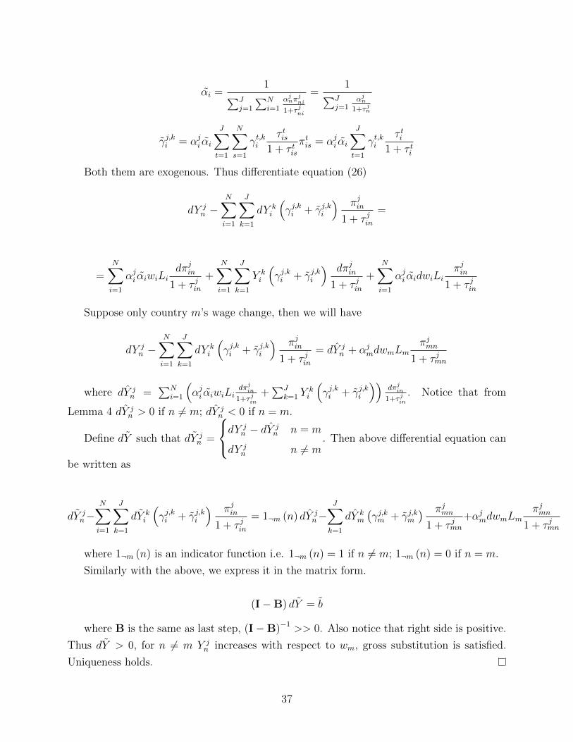
αi =1∑J

j=1

∑Ni=1

αjnπjni

1+τ jni

=1∑J

j=1αjn

1+τ jn

γj,ki = αji αi

J∑t=1

N∑s=1

γt,kiτ tis

1 + τ tisπtis = αji αi

J∑t=1

γt,kiτ ti

1 + τ ti

Both them are exogenous. Thus differentiate equation (26)

dY jn −

N∑i=1

J∑k=1

dY ki

(γj,ki + γj,ki

) πjin1 + τ jin

=

=N∑i=1

αji αiwiLidπjin

1 + τ jin+

N∑i=1

J∑k=1

Y ki

(γj,ki + γj,ki

) dπjin1 + τ jin

+N∑i=1

αji αidwiLiπjin

1 + τ jin

Suppose only country m’s wage change, then we will have

dY jn −

N∑i=1

J∑k=1

dY ki

(γj,ki + γj,ki

) πjin1 + τ jin

= dY jn + αjmdwmLm

πjmn1 + τ jmn

where dY jn =

∑Ni=1

(αji αiwiLi

dπjin1+τ jin

+∑J

k=1 Yki

(γj,ki + γj,ki

))dπjin

1+τ jin. Notice that from

Lemma 4 dY jn > 0 if n 6= m; dY j

n < 0 if n = m.

Define dY such that dY jn =

dY jn − dY j

n n = m

dY jn n 6= m

. Then above differential equation can

be written as

dY jn−

N∑i=1

J∑k=1

dY ki

(γj,ki + γj,ki

) πjin1 + τ jin

= 1¬m (n) dY jn−

J∑k=1

dY km

(γj,km + γj,km

) πjmn1 + τ jmn

+αjmdwmLmπjmn

1 + τ jmn

where 1¬m (n) is an indicator function i.e. 1¬m (n) = 1 if n 6= m; 1¬m (n) = 0 if n = m.

Similarly with the above, we express it in the matrix form.

(I−B) dY = b

where B is the same as last step, (I−B)−1 >> 0. Also notice that right side is positive.

Thus dY > 0, for n 6= m Y jn increases with respect to wm, gross substitution is satisfied.

Uniqueness holds.

37

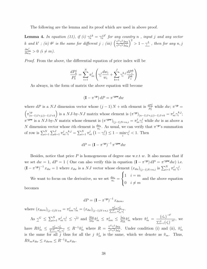
The following are the lemma and its proof which are used in above proof.

Lemma 4. In equation (11), if (i) γj,kn = γj,k′

n for any country n , input j and any sector

k and k′ ; (ii) θj is the same for different j ; (iii)(γGγLλκθ

γGγLλκθ

)2

> 1 − γL , then for any n, j

∂πjni∂wm

> 0 (i 6= m).

Proof. From the above, the differential equation of price index will be

dP jn

P jn

=N∑i=1

πjni

(γjidwiwi

+J∑k=1

γk,jidP k

i

P ki

)As always, in the form of matrix the above equation will become

(I− πγp) dP = πγpwdw

where dP is a NJ dimension vector whose (j − 1)N + nth element is dP jnP jn

while dw; πγp =(πγp(n−1)J+j,(i−1)J+k

)is a NJ-by-NJ matrix whose element is (πγp)(n−1)J+j,(i−1)J+k = πjniγ

k,ji ;

πγpw is a NJ-by-N matrix whose element is (πγpw)(j−1)N+n,i = πjniγji while dw is as above a

N dimension vector whose ith element is dwiwi

. As usual, we can verify that πγp’s summation

of row is∑N

i=1

∑Jk=1 π

jniγ

k,ji =

∑Ni=1 π

jni

(1− γji

)≤ 1−min

iγji < 1. Then

dP = (I− πγp)−1 πγpwdw

Besides, notice that price P is homogeneous of degree one w.r.t w. It also means that if

we set dw = 1, dP = 1 ( One can also verify this in equation (I− πγp) dP = πγpwdw) i.e.

(I− πγp)−1 xdw = 1 where xdw is a NJ vector whose element (xdw)(j−1)N+n,i is∑N

i=1 πjniγ

ji .

We want to focus on the derivative, so we set dwiwi

=

1 i = m

0 i 6= mand the above equation

becomes

dP = (I− πγp)−1 xdwm,

where (xdwm)(j−1)N+n = πjnmγjm = (xdw)(j−1)N+n,i

πjnmγjm∑N

i=1 πjniγ

ji

.

As γG ≤∑N

i=1 πjniγ

ji ≤ γG and

λκθλκθ

πjm ≤ πjnm ≤ λκθλκθ

πjm where πjm =(cjm)

−θj

∑Nh=1(c

jh)−θj , we

have Rπjm ≤πjnmγ

jm∑N

i=1 πjniγ

ji

≤ R−1πjm where R =γGγLλκθ

γGγLλκθ. Under condition (i) and (ii), πjm

is the same for all j thus for all the j πjm is the same, which we denote as πm. Thus,

Rπmxdw ≤ xdwm ≤ R−1πmxdw.

38

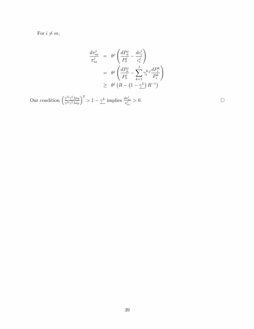
For i 6= m,

dπjniπjni

= θj

(dP j

n

P jn

− dcjicji

)

= θj

(dP j

n

P jn

−J∑k=1

γk,jidP k

i

P ki

)≥ θj

(R−

(1− γL

)R−1

)Our condition

(γGγLλκθ

γGγLλκθ

)2

> 1− γL impliesdπjniπjni

> 0.

39