On the Expressive Power of Deep Learning: A Tensor Analysisproceedings.mlr.press/v49/cohen16.pdf · ON THE EXPRESSIVE POWER OF DEEP LEARNING: A TENSOR ANALYSIS ing that the amount

JMLR: Workshop and Conference Proceedings vol 49:1–31, 2016

On the Expressive Power of Deep Learning: A Tensor Analysis

Nadav Cohen [email protected]

Or Sharir [email protected]

Amnon Shashua [email protected]

The Hebrew University of Jerusalem

AbstractIt has long been conjectured that hypotheses spaces suitable for data that is compositional in

nature, such as text or images, may be more efficiently represented with deep hierarchical networksthan with shallow ones. Despite the vast empirical evidence supporting this belief, theoreticaljustifications to date are limited. In particular, they do not account for the locality, sharing andpooling constructs of convolutional networks, the most successful deep learning architecture todate. In this work we derive a deep network architecture based on arithmetic circuits that inherentlyemploys locality, sharing and pooling. An equivalence between the networks and hierarchicaltensor factorizations is established. We show that a shallow network corresponds to CP (rank-1)decomposition, whereas a deep network corresponds to Hierarchical Tucker decomposition. Usingtools from measure theory and matrix algebra, we prove that besides a negligible set, all functionsthat can be implemented by a deep network of polynomial size, require exponential size in order tobe realized (or even approximated) by a shallow network. Since log-space computation transformsour networks into SimNets, the result applies directly to a deep learning architecture demonstratingpromising empirical performance. The construction and theory developed in this paper shed newlight on various practices and ideas employed by the deep learning community.

Keywords: Deep Learning, Expressive Power, Arithmetic Circuits, Tensor Decompositions

1. Introduction

The expressive power of neural networks is achieved through depth. There is mounting empiricalevidence that for a given budget of resources (e.g. neurons), the deeper one goes, the better theeventual performance will be. However, existing theoretical arguments that support this empiricalfinding are limited. There have been many attempts to theoretically analyze function spaces gen-erated by network architectures, and their dependency on network depth and size. The prominentapproach for justifying the power of depth is to show that deep networks can efficiently expressfunctions that would require shallow networks to have super-polynomial size. We refer to suchscenarios as instances of depth efficiency. Unfortunately, existing results dealing with depth effi-ciency (e.g. Hastad (1986); Hastad and Goldmann (1991); Delalleau and Bengio (2011); Martensand Medabalimi (2014)) typically apply to specific network architectures that do not resemble onescommonly used in practice. In particular, none of these results apply to convolutional networks(LeCun and Bengio (1995)), which represent the most empirically successful and widely used deeplearning architecture to date. A further limitation of current results is that they merely show ex-istence of depth efficiency (i.e. of functions that are efficiently realizable with a certain depth butcannot be efficiently realized with shallower depths), without providing any information as to howfrequent this property is. These shortcomings of current theory are the ones that motivated our work.

c© 2016 N. Cohen, O. Sharir & A. Shashua.

COHEN SHARIR SHASHUA

The architectural features that specialize convolutional networks compared to classic feed-forward fully-connected networks are threefold. The first feature, locality, refers to the connectionof a neuron only to neighboring neurons in the preceding layer, as opposed to having the entirelayer drive it. In the context of image processing (the most common application of convolutionalnetworks), locality is believed to reflect the inherent compositional structure of data – the closerpixels are in an image, the more likely they are to be correlated. The second architectural feature ofconvolutional networks is sharing, which means that different neurons in the same layer, connectedto different neighborhoods in the preceding layer, share the same weights. Sharing, which togetherwith locality gives rise to convolution, is motivated by the fact that in natural images, the semanticmeaning of a pattern often does not depend on its location (i.e. two identical patterns appearing indifferent locations of an image often convey the same semantic content). Finally, the third archi-tectural idea of convolutional networks is pooling, which is essentially an operator that decimateslayers, replacing neural activations in a spatial window by a single value (e.g. their maximum oraverage). In the context of images, pooling induces invariance to translations (which often do notaffect semantic content), and in addition is believed to create a hierarchy of abstraction in the pat-terns neurons respond to. The three architectural elements of locality, sharing and pooling, whichhave facilitated the great success of convolutional networks, are all lacking in existing theoreticalstudies of depth efficiency.

In this paper we introduce a convolutional arithmetic circuit architecture that incorporates lo-cality, sharing and pooling. Arithmetic circuits (also known as Sum-Product Networks, Poon andDomingos (2011)) are networks with two types of nodes: sum nodes, which compute a weightedsum of their inputs, and product nodes, computing the product of their inputs. We use sum nodes toimplement convolutions (locality with sharing), and product nodes to realize pooling. The modelswe arrive at may be viewed as convolutional networks with product pooling and linear point-wise ac-tivation. They are attractive on three accounts. First, as discussed in app. E, convolutional arithmeticcircuits are equivalent to SimNets, a new deep learning architecture that has recently demonstratedpromising empirical results on various image recognition benchmarks (Cohen et al. (2016)). Sec-ond, as we show in sec. 3, convolutional arithmetic circuits are realizations of hierarchical tensordecompositions (see Hackbusch (2012)), opening the door to various mathematical and algorithmictools for their analysis and implementation. Third, the depth efficiency of convolutional arithmeticcircuits, which we analyze in sec. 4, was shown in the subsequent work of Cohen and Shashua(2016) to be superior to the depth efficiency of the popular convolutional rectifier networks, namelyconvolutional networks with rectified linear (ReLU) activation and max or average pooling.

Employing machinery from measure theory and matrix algebra, made available through theirconnection to hierarchical tensor decompositions, we prove a number of fundamental results con-cerning the depth efficiency of our convolutional arithmetic circuits. Our main theoretical result(thm. 1 and corollary 2) states that besides a negligible (zero measure) set, all functions that canbe realized by a deep network of polynomial size, require exponential size in order to be realized,or even approximated, by a shallow network. When translated to the viewpoint of tensor decom-positions, this implies that almost all tensors realized by Hierarchical Tucker (HT) decomposition(Hackbusch and Kuhn (2009)) cannot be efficiently realized by the classic CP (rank-1) decompo-sition. To the best of our knowledge, this result is unknown to the tensor analysis community, inwhich the advantage of HT over CP is typically demonstrated through specific examples of tensorsthat can be efficiently realized by the former and not by the latter. Following our main result, wepresent a generalization (thm. 3 and corollary 4) that compares networks of arbitrary depths, show-

2

ON THE EXPRESSIVE POWER OF DEEP LEARNING: A TENSOR ANALYSIS

ing that the amount of resources one has to pay in order to maintain representational power whiletrimming down layers of a network grows double exponentially w.r.t. the number of layers cut off.We also characterize cases in which dropping a single layer bears an exponential price.

The remainder of the paper is organized as follows. In sec. 2 we briefly review notations andmathematical background required in order to follow our work. This is followed by sec. 3, whichpresents our convolutional arithmetic circuits and establishes their equivalence with tensor decom-positions. Our theoretical analysis is covered in sec. 4. Finally, sec. 5 concludes. In order to keepthe manuscript at a reasonable length, we defer our detailed survey of related work to app. D, cov-ering works on the depth efficiency of boolean circuits, arithmetic circuits and neural networks, aswell as different applications of tensor analysis in the field of deep learning.

2. Preliminaries

We begin by establishing notational conventions that will be used throughout the paper. We denotevectors using bold typeface, e.g. v ∈ Rs. The coordinates of such a vector are referenced withregular typeface and a subscript, e.g. vi ∈ R. This is not to be confused with bold typeface and asubscript, e.g. vi ∈ Rs, which represents a vector that belongs to some sequence. Tensors (multi-dimensional arrays) are denoted by the letters “A” and “B” in calligraphic typeface, e.g. A,B ∈RM1×···×MN . A specific entry in a tensor will be referenced with subscripts, e.g. Ad1...dN ∈ R.Superscripts will be used to denote individual objects within a collection. For example, v(i) standsfor vector i and Ay stands for tensor y. In cases where the collection of interest is indexed bymultiple coordinates, we will have multiple superscripts referencing individual objects, e.g. al,j,γ

will stand for vector (l, j, γ). As shorthand for the Cartesian product of the Euclidean space Rs withitselfN times, we will use the notation (Rs)N . Finally, for a positive integer k we use the shorthand[k] to denote the set 1, . . . , k.

We now turn to establish a baseline, i.e. to present basic definitions and results, in the broad andcomprehensive field of tensor analysis. We list here only the essentials required in order to followthe paper, referring the interested reader to Hackbusch (2012) for a more complete introduction tothe field 1. The most straightforward way to view a tensor is simply as a multi-dimensional array:Ad1,...,dN ∈ R where i ∈ [N ], di ∈ [Mi]. The number of indexing entries in the array, which arealso called modes, is referred to as the order of the tensor. The term dimension stands for the numberof values an index can take in a particular mode. For example, the tensor A appearing above hasorder N and dimension Mi in mode i, i ∈ [N ]. The space of all possible configurations A can takeis called a tensor space and is denoted, quite naturally, by RM1×···×MN .

A central operator in tensor analysis is the tensor product, denoted ⊗. This operator intakestwo tensors A and B of orders P and Q respectively, and returns a tensor A ⊗ B of order P + Q,defined by: (A⊗ B)d1...dP+Q

= Ad1...dP · BdP+1...dP+Q. Notice that in the case P = Q = 1, the

tensor product reduces to an outer product between vectors. Specifically, v⊗u – the tensor productbetween u ∈ RM1 and v ∈ RM2 , is no other than the rank-1 matrix vu> ∈ RM1×M2 . In thiscontext, we will often use the shorthand⊗Ni=1 v

(i) to denote the joint tensor product v(1)⊗· · ·⊗v(N).Tensors of the form ⊗Ni=1 v

(i) are called pure or elementary, and are regarded as having rank-1(assuming v(i) 6= 0 ∀i). It is not difficult to see that any tensor can be expressed as a sum of rank-1

1. The definitions we give are concrete special cases of the more abstract algebraic definitions given in Hackbusch(2012). We limit the discussion to these special cases since they suffice for our needs and are easier to grasp.

3


tensors:

A =

Z∑z=1

v(1)z ⊗ · · · ⊗ v(N)

z ,v(i)z ∈ RMi (1)

A representation as above is called a CANDECOMP/PARAFAC decomposition of A, or in short,a CP decomposition 2. The CP-rank of A is defined as the minimum number of terms in a CPdecomposition, i.e. as the minimal Z for which eq. 1 can hold. Notice that for a tensor of order 2,i.e. a matrix, this definition of CP-rank coincides with that of standard matrix rank.

A symmetric tensor is one that is invariant to permutations of its indices. Formally, a ten-sor A of order N which is symmetric will have equal dimension M in all modes, and for ev-ery permutation π : [N ] → [N ] and indices d1. . .dN ∈ [M ], the following equality will hold:Adπ(1)...dπ(N)

= Ad1...dN . Note that for a vector v ∈ RM , the tensor ⊗Ni=1 v ∈ RM×···×M issymmetric. Moreover, every symmetric tensor may be expressed as a linear combination of such(symmetric rank-1) tensors: A =

∑Zz=1 λz · vz ⊗ · · · ⊗ vz . This is referred to as a symmetric CP

decomposition, and the symmetric CP-rank is the minimal Z for which such a decomposition exists.Since a symmetric CP decomposition is in particular a standard CP decomposition, the symmetricCP-rank of a symmetric tensor is always greater or equal to its standard CP-rank. Note that for thecase of symmetric matrices (order-2 tensors) the symmetric CP-rank and the original CP-rank arealways equal.

A repeating concept in this paper is that of measure zero. More broadly, our analysis is framedin measure theoretical terms. While an introduction to the field is beyond the scope of the paper (theinterested reader is referred to Jones (2001)), it is possible to intuitively grasp the ideas that form thebasis to our claims. When dealing with subsets of a Euclidean space, the standard and most naturalmeasure in a sense is called the Lebesgue measure. This is the only measure we consider in ouranalysis. A set of (Lebesgue) measure zero can be thought of as having zero “volume” in the spaceof interest. For example, the interval between (0, 0) and (1, 0) has zero measure as a subset of the2D plane, but has positive measure as a subset of the 1D x-axis. An alternative way to view a zeromeasure set S follows the property that if one draws a random point in space by some continuousdistribution, the probability of that point hitting S is necessarily zero. A related term that will beused throughout the paper is almost everywhere, which refers to an entire space excluding, at most,a set of zero measure.

3. Convolutional Arithmetic Circuits

We consider the task of classifying an instance X = (x1, . . . ,xN ), xi ∈ Rs, into one of thecategories Y := 1, . . . , Y . Representing instances as collections of vectors is natural in manyapplications. In the case of image processing for example, X may correspond to an image, andx1 . . .xN may correspond to vector arrangements of (possibly overlapping) patches around pix-els. As customary, classification is carried out through maximization of per-label score func-tions hyy∈Y , i.e. the predicted label for the instance X will be the index y ∈ Y for which thescore value hy(X) is maximal. Our attention is thus directed to functions over the instance spaceX := (x1, . . . ,xN ) : xi ∈ Rs = (Rs)N . We define our hypotheses space through the following

2. CP decomposition is regarded as the classic and most basic tensor decomposition, dating back to the beginning ofthe 20’th century (see Kolda and Bader (2009) for a historic survey).

4


,d irep i d f x

input representation 1x1 conv

global pooling

dense (output)

hidden layer

ix

M Z Z Y

,, , ,:z iconv i z rep i a

1

,N

ipool z conv i z

, :yout y pool a

X

Figure 1: CP model – convolutional arithmetic circuit implementing CP (rank-1) decomposition.

representation of score functions:

hy (x1, . . . ,xN ) =M∑

d1...dN=1

Ayd1,...,dNN∏i=1

fθdi (xi) (2)

fθ1 . . .fθM : Rs → R are referred to as representation functions, selected from a parametric familyF = fθ : Rs → Rθ∈Θ. Natural choices for this family are wavelets, radial basis functions (Gaus-sians), and affine functions followed by point-wise activation (neurons). The coefficient tensor Ayhas order N and dimension M in each mode. Its entries correspond to a basis of MN point-wiseproduct functions (x1, . . . ,xN ) 7→

∏Ni=1 fθdi (xi)d1...dN∈[M ]. We will often consider fixed lin-

early independent representation functions fθ1 . . .fθM . In this case the point-wise product functionsare linearly independent as well (see app. C.1), and we have a one to one correspondence betweenscore functions and coefficient tensors. To keep the manuscript concise, we defer the derivation ofour hypotheses space (eq. 2) to app. C, noting here that it arises naturally from the notion of tensorproducts between L2 spaces.

Our eventual aim is to realize score functions hy with a layered network architecture. As afirst step along this path, we notice that hy(x1, . . . ,xN ) is fully determined by the activations ofthe M representation functions fθ1 . . .fθM on the N input vectors x1. . .xN . In other words, givenfθd(xi)d∈[M ],i∈[N ], the score hy(x1, . . . ,xN ) is independent of the input. It is thus natural to con-sider the computation of these M ·N numbers as the first layer of our networks. This layer, referredto as the representation layer, may be conceived as a convolutional operator with M channels, eachcorresponding to a different function applied to all input vectors (see fig. 1).

Once we have constrained our score functions to have the structure depicted in eq. 2, learninga classifier reduces to estimation of the parameters θ1. . .θM , and the coefficient tensors A1. . .AY .The computational challenge is that the latter tensors are of order N (and dimension M in eachmode), having an exponential number of entries (MN each). In the next subsections we utilizetensor decompositions (factorizations) to address this computational challenge, and show how theyare naturally realized by convolutional arithmetic circuits.

5


3.1. Shallow Network as a CP Decomposition of Ay

The most straightforward way to factorize a tensor is through a CP (rank-1) decomposition (seesec. 2). Consider a joint CP decomposition for the coefficient tensors Ayy∈Y :

Ay =Z∑z=1

ayz · az,1 ⊗ · · · ⊗ az,N (3)

where ay ∈ RZ for y ∈ Y (ayz stands for entry z of ay), and az,i ∈ RM for i ∈ [N ], z ∈ [Z]. Thedecomposition is joint in the sense that the same vectors az,i are shared across all classes y. Clearly,if we set Z = MN this model is universal, i.e. any tensors A1. . .AY may be represented.

Substituting our CP decomposition (eq. 3) into the expression for the score functions in eq. 2,we obtain:

hy(X) =

Z∑z=1

ayz

N∏i=1

(M∑d=1

az,id fθd(xi)

)From this we conclude that the network illustrated in fig. 1 implements a classifier (score functions)under the CP decomposition in eq. 3. We refer to this network as CP model. The network consistsof a representation layer followed by a single hidden layer, which in turn is followed by the output.The hidden layer begins with a 1 × 1 conv operator, which is simply a 3D convolution with Zchannels and receptive field 1× 1. The convolution may operate without coefficient sharing, i.e. thefilters that generate feature maps by sliding across the previous layer may have different coefficientsat different spatial locations. This is often referred to in the deep learning community as a locally-connected operator (see Taigman et al. (2014)). To obtain a standard convolutional operator, simplyenforce coefficient sharing by constraining the vectors az,i in the CP decomposition (eq. 3) to beequal to each other for different values of i (this setting is discussed in sec. 3.3). Following convoperator, the hidden layer includes global product pooling. Feature maps generated by conv arereduced to singletons through multiplication of their entries, creating a vector of dimension Z. Thisvector is then mapped into the Y network outputs through a final dense linear layer.

To recap, CP model (fig. 1) is a shallow (single hidden layer) convolutional arithmetic circuitthat realizes the CP decomposition (eq. 3). It is universal, i.e. it can realize any coefficient tensorswith large enough size (Z). Unfortunately, since the CP-rank of a generic tensor is exponential inits order (see Hackbusch (2012)), the size required for CP model to be universal is exponential (Zexponential in N ).

3.2. Deep Network as a Hierarchical Decomposition of Ay

In this subsection we present a deep network that corresponds to the recently introduced Hierar-chical Tucker tensor decomposition (Hackbusch and Kuhn (2009)), which we refer to in short asHT decomposition. The network, dubbed HT model, is universal. Specifically, any set of tensorsAy represented by CP model can be represented by HT model with only a polynomial penalty interms of resources. The advantage of HT model, as we show in sec. 4, is that in almost all casesit generates tensors that require an exponential size in order to be realized, or even approximated,by CP model. Put differently, if one draws the weights of HT model by some continuous distribu-tion, with probability one, the resulting tensors cannot be approximated by a polynomial CP model.Informally, this implies that HT model is exponentially more expressive than CP model.

6


,d irep i d f x

input representation 1x1 convpooling

1x1 convpooling

dense (output)

hidden layer 0 hidden layer L-1(L=log2N)

ix

M 0r 0r 1Lr 1Lr Y

0, ,

0 , , ,:jconv j rep j a

0 0

' 2 1,2

, ',j j j

pool j conv j

1 1

' 1,2

',L L

j

pool conv j

,

1, :L y

Lout y pool a

X

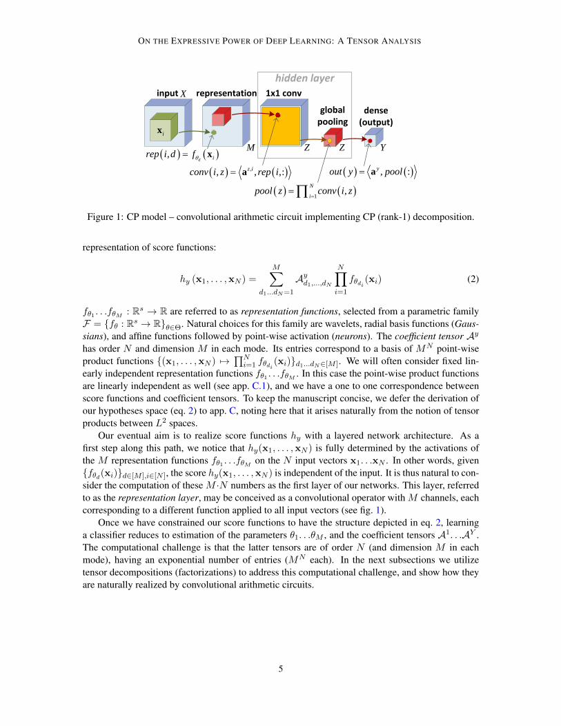
Figure 2: HT model – convolutional arithmetic circuit implementing hierarchical decomposition.

HT model is based on the hierarchical tensor decomposition in eq. 4, which is a special caseof the HT decomposition as presented in Hackbusch and Kuhn (2009) (in the latter’s terminology,we restrict the matrices Al,j,γ to be diagonal). Our construction and theoretical results apply to thegeneral HT decomposition as well, with the specialization done merely to bring forth a network thatresembles current convolutional networks 3.

φ1,j,γ =

r0∑α=1

a1,j,γα a0,2j−1,α ⊗ a0,2j,α

· · ·

φl,j,γ =

rl−1∑α=1

al,j,γα φl−1,2j−1,α︸︷︷︸order 2l−1

⊗φl−1,2j,α︸︷︷︸order 2l−1

· · ·

φL−1,j,γ =

rL−2∑α=1

aL−1,j,γα φL−2,2j−1,α︸︷︷︸

order N4

⊗φL−2,2j,α︸︷︷︸order N

4

Ay =

rL−1∑α=1

aL,yα φL−1,1,α︸︷︷︸order N

2

⊗φL−1,2,α︸︷︷︸order N

2

(4)

The decomposition in eq. 4 recursively constructs the coefficient tensors Ayy∈[Y ] by assem-bling vectors a0,j,γj∈[N ],γ∈[r0] into tensors φl,j,γl∈[L−1],j∈[N/2l],γ∈[rl]

in an incremental fashion.The index l stands for the level in the decomposition, j represents the “location” within level l, andγ corresponds to the individual tensor in level l and location j. rl is referred to as level-l rank,and is defined to be the number of tensors in each location of level l (we denote for completenessrL := Y ). The tensor φl,j,γ has order 2l, and we assume for simplicity that N – the order of Ay,is a power of 2 (this is merely a technical assumption also made in Hackbusch and Kuhn (2009), itdoes not limit the generality of our analysis).

The parameters of the decomposition are the final level weights aL,y ∈ RrL−1y∈[Y ], the in-termediate levels’ weights al,j,γ ∈ Rrl−1l∈[L−1],j∈[N/2l],γ∈[rl]

, and the first level vectors a0,j,γ ∈RMj∈[N ],γ∈[r0]. This totals at N · M · r0 +

∑L−1l=1

N2l· rl−1 · rl + Y · rl−1 individual parame-

3. If we had not constrained Al,j,γ to be diagonal, pooling operations would involve entries from different channels.

7


ters, and if we assume equal ranks r := r0 = · · · = rL−1, the number of parameters becomesN ·M · r +N · r2 + Y · r.

The hierarchical decomposition (eq. 4) is universal, i.e. with large enough ranks rl it can rep-resent any tensors. Moreover, it is a super-set of the CP decomposition (eq. 3). That is to say,all tensors representable by a CP decomposition having Z components are also representable by ahierarchical decomposition with ranks r0 = r1 = · · · = rL−1 = Z 4. Note that this comes witha polynomial penalty – the number of parameters increases from N · M · Z + Z · Y in the CPdecomposition, to N ·M · Z + Z · Y +N · Z2 in the hierarchical decomposition. However, as weshow in sec. 4, the gain in expressive power is exponential.

Plugging the expression forAy in our hierarchical decomposition (eq. 4) into the score functionhy given in eq. 2, we obtain the network displayed in fig. 2 – HT model. This network includes arepresentation layer followed by L = log2N hidden layers which in turn are followed by the output.As in the shallow CP model (fig. 1), the hidden layers consist of 1 × 1 conv operators followed byproduct pooling. The difference is that instead of a single hidden layer collapsing the entire spatialstructure through global pooling, hidden layers now pool over size-2 windows, decimating featuremaps by a factor of two (no overlaps). After L = log2N such layers feature maps are reduced tosingletons, and we arrive at a 1D structure with rL−1 nodes. This is then mapped into Y networkoutputs through a final dense linear layer. We note that the network’s size-2 pooling windows (andthe resulting number of hidden layers L = log2N ) correspond to the fact that our hierarchicaldecomposition (eq. 4) is based on a full binary tree over modes, i.e. it combines (through tensorproduct) two tensors at a time. We focus on this setting solely for simplicity of presentation, andsince it is the one presented in Hackbusch and Kuhn (2009). Our analysis (sec. 4) could easily beadapted to hierarchical decompositions based on other trees (taking tensor products between morethan two tensors at a time), and that would correspond to networks with different pooling windowsizes and resulting depths.

HT model (fig. 2) is conceptually divided into two parts. The first is the representation layer,transforming input vectors x1. . .xN into N ·M real-valued scalars fθd(xi)i∈[N ],d∈[M ]. The sec-ond and main part of the network, which we view as an “inference” engine, is the convolutionalarithmetic circuit that takes the N ·M measurements produced by the representation layer, and ac-cordingly computes Y class scores at the output layer.

To recap, we have now a deep network (fig. 2), which we refer to as HT model, that computesthe score functions hy (eq. 2) with coefficient tensors Ay hierarchically decomposed as in eq. 4.The network is universal in the sense that with enough channels rl, any tensors may be represented.Moreover, the model is a super-set of the shallow CP model presented in sec. 3.1. The question ofdepth efficiency now naturally arises. In particular, we would like to know if there are functions thatmay be represented by a polynomially sized deep HT model, yet require exponential size from theshallow CP model. The answer, as described in sec. 4, is that almost all functions realizable by HTmodel meet this property. In other words, the set of functions realizable by a polynomial CP modelhas measure zero in the space of functions realizable by a given polynomial HT model.

4. To see this, simply assign the first level vectors a0,j,γ with CP’s basis vectors, the last level weights with CP’sper-class weights, and the intermediate levels’ weights with indicator vectors.

8


3.3. Shared Coefficients for Convolution

The 1× 1 conv operator in our networks (see fig. 1 and 2) implements a local linear transformationwith coefficients generally being location-dependent. In the special case where coefficients do notdepend on location, i.e. remain fixed across space, the local linear transformation becomes a stan-dard convolution. We refer to this setting as coefficient sharing. Sharing is a widely used structuralconstraint, one of the pillars behind the successful convolutional network architecture. In the con-text of image processing (prominent application of convolutional networks), sharing is motivated bythe observation that in natural images, the semantic content of a pattern often does not depend on itslocation. In this subsection we explore the effect of sharing on the expressiveness of our networks,or more specifically, on the coefficient tensors Ay they can represent.

For CP model, coefficient sharing amounts to setting az := az,1 = · · · = az,N in the CPdecomposition (eq. 3), transforming the latter to a symmetric CP decomposition:

Ay =

Z∑z=1

ayz · az ⊗ · · · ⊗ az︸︷︷︸N times

,az ∈ RM ,ay ∈ RZ

CP model with sharing is not universal (not all tensors Ay are representable, no matter how large Zis allowed to be) – it can only represent symmetric tensors.

In the case of HT model, sharing amounts to applying the following constraints on the hierarchi-cal decomposition in eq. 4: al,γ := al,1,γ = · · · = al,N/2

l,γ for every l = 0. . .L− 1 and γ = 1. . .rl.Note that in this case universality is lost as well, but nonetheless generated tensors are not limitedto be symmetric, already demonstrating an expressive advantage of deep models over shallow ones.In sec. 4 we take this further by showing that the shared HT model is exponentially more expressivethan CP model, even if the latter is not constrained by sharing.

4. Theorems of Network Capacity

The first contribution of this paper, presented in sec. 3, is the equivalence between deep learningarchitectures successfully employed in practice, and tensor decompositions. Namely, we showedthat convolutional arithmetic circuits as in fig. 2, which are in fact SimNets that have demonstratedpromising empirical performance (see app. E), may be formulated as hierarchical tensor decompo-sitions. As a second contribution, we make use of the established link between arithmetic circuitsand tensor decompositions, combining theoretical tools from these two worlds, to prove results thatare of interest to both deep learning and tensor analysis communities. This is the focus of the currentsection.

The fundamental theoretical result proven in this paper is the following:

Theorem 1 Let Ay be a tensor of order N and dimension M in each mode, generated by therecursive formulas in eq. 4. Define r := minr0,M, and consider the space of all possibleconfigurations for the parameters of the composition – al,j,γl,j,γ . In this space, the generatedtensor Ay will have CP-rank of at least rN/2 almost everywhere (w.r.t. Lebesgue measure). Putdifferently, the configurations for which the CP-rank of Ay is less than rN/2 form a set of measurezero. The exact same result holds if we constrain the composition to be “shared”, i.e. set al,j,γ ≡al,γ and consider the space of al,γl,γ configurations.

From the perspective of deep learning, thm. 1 leads to the following corollary:

9


Corollary 2 Given linearly independent representation functions fθdd∈[M ], randomizing theweights of HT model (sec. 3.2) by a continuous distribution induces score functions hy that withprobability one, cannot be approximated arbitrarily well (in L2 sense) by a CP model (sec. 3.1)with less than minr0,MN/2 hidden channels. This result holds even if we constrain HT modelwith weight sharing (sec. 3.3) while leaving CP model in its general form.

That is to say, besides a negligible set, all functions that can be realized by a polynomially sizedHT model (with or without weight sharing), require exponential size in order to be realized, or evenapproximated, by CP model. Most of the previous works relating to depth efficiency (see app. D)merely show existence of functions that separate depths (i.e. that are efficiently realizable by a deepnetwork yet require super-polynomial size from shallow networks). Corollary 2 on the other handestablishes depth efficiency for almost all functions that a deep network can implement. Equallyimportantly, it applies to deep learning architectures that are being successfully employed in practice(SimNets – see app. E).

Adopting the viewpoint of tensor analysis, thm. 1 states that besides a negligible set, all tensorsrealized by HT (Hierarchical Tucker) decomposition cannot be represented by the classic CP (rank-1) decomposition if the latter has less than an exponential number of terms 5. To the best of ourknowledge, this result has never been proved in the tensor analysis community. In the originalpaper introducing HT decomposition (Hackbusch and Kuhn (2009)), as a motivating example, theauthors present a specific tensor that is efficiently realizable by HT decomposition while requiringan exponential number of terms from CP decomposition 6. Our result strengthens this motivationconsiderably, showing that it is not just one specific tensor that favors HT over CP, but rather, almostall tensors realizable by HT exhibit this preference. Taking into account that any tensor realized byCP can also be realized by HT with only a polynomial penalty in the number of parameters (seesec. 3.2), this implies that in an asymptotic sense, HT decomposition is exponentially more efficientthan CP decomposition.

4.1. Proof Sketches

The complete proofs of thm. 1 and corollary 2 are given in app. B. We provide here an outline ofthe main tools employed and arguments made along these proofs.

To prove thm. 1 we combine approaches from the worlds of circuit complexity and tensor de-compositions. The first class of machinery we employ is matrix algebra, which has proven to be apowerful source of tools for analyzing the complexity of circuits. For example, arithmetic circuitshave been analyzed through what is called the partial derivative matrix (see Raz and Yehudayoff(2009)), and for boolean circuits a widely used tool is the communication matrix (see Karchmer(1989)). We gain access to matrix algebra by arranging tensors that take part in the CP and HTdecompositions as matrices, a process often referred to as matricization. With matricization, thetensor product translates to the Kronecker product, and the properties of the latter become readilyavailable. The second tool-set we make use of is measure theory, which prevails in the study of ten-sor decompositions, but is much less frequent in analyses of circuit complexity. In order to frame

5. As stated in sec. 3.2, the decomposition in eq. 4 to which thm. 1 applies is actually a special case of HT decompositionas introduced in Hackbusch and Kuhn (2009). However, the theorem and its proof can easily be adapted to accountfor the general case. We focus on the special case merely because it corresponds to convolutional arithmetic circuitarchitectures used in practice.

6. The same motivating example is given in a more recent textbook introducing tensor analysis (Hackbusch (2012)).

10


a problem in measure theoretical terms, one obviously needs to define a measure space of inter-est. For tensor decompositions, the straightforward space to focus on is that of the decompositionvariables. For general circuits on the other hand, it is often unclear if defining a measure space isat all appropriate. However, when circuits are considered in the context of machine learning theyare usually parameterized, and defining a measure space on top of these parameters is an effectiveapproach for studying the prevalence of various properties in hypotheses spaces.

Our proof of thm. 1 traverses through the following path. We begin by showing that matricizinga rank-1 tensor produces a rank-1 matrix. This implies that the matricization of a tensor generated bya CP decomposition with Z terms has rank at most Z. We then turn to show that the matricizationof a tensor generated by the HT decomposition in eq. 4 has rank at least minr0,MN/2 almosteverywhere. This is done through induction over the levels of the decomposition (l = 1. . .L). Forthe first level (l = 1), we use a combination of measure theoretical and linear algebraic argumentsto show that the generated matrices have maximal rank (minr0,M) almost everywhere. For theinduction step, the facts that under matricization tensor product translates into Kronecker product,and that the latter increases ranks multiplicatively 7, imply that matricization ranks in the currentlevel are generally equal to those in the previous level squared. Measure theoretical claims are thenmade to ensure that this indeed takes place almost everywhere.

To prove corollary 2 based on thm. 1, we need to show that the inability of CP model to realize atensor generated by HT model, implies that the former cannot approximate score functions producedby the latter. In general, the set of tensors expressible by a CP decomposition is not topologicallyclosed 8, which implies that a-priori, it may be that CP model can approximate tensors generatedby HT model even though it cannot realize them. However, since the proof of thm. 1 was achievedthrough separation of matrix rank, distances are indeed positive and CP model cannot approximateHT model’s tensors almost always. To translate from tensors to score functions, we simply notethat in a finite-dimensional Hilbert space convergence in norm implies convergence in coefficientsunder any basis. Therefore, in the space of score functions (eq. 2) convergence in norm impliesconvergence in coefficients under the basis (x1, . . . ,xN )7→

∏Ni=1 fθdi (xi)d1...dN∈[M ]. That is to

say, it implies convergence in coefficient tensors.

4.2. Generalization

Thm. 1 and corollary 2 compare the expressive power of the deep HT model (sec. 3.2) to that ofthe shallow CP model (sec. 3.1). One may argue that such an analysis is lacking, as it does notconvey information regarding the importance of each individual layer. In particular, it does not shedlight on the advantage of very deep networks, which at present provide state of the art recognitionaccuracy, compared to networks of more moderate depth. For this purpose we present a generaliza-tion, specifying the amount of resources one has to pay in order to maintain representational powerwhile layers are incrementally cut off from a deep network. For conciseness we defer this analysisto app. A, and merely state here our final conclusions. We find that the representational penalty isdouble exponential w.r.t. the number of layers removed. In addition, there are certain cases wherethe removal of even a single layer leads to an exponential inflation, falling in line with the suggestionof Bengio (2009).

7. If denotes the Kronecker product, then for any matrices A and B: rank(AB) = rank(A)·rank(B).8. Hence the definition of border rank, see Hackbusch (2012).

11


5. Discussion

In this work we address a fundamental issue in deep learning – the expressive efficiency of depth.There have been many attempts to theoretically analyze this question, but from a practical machinelearning perspective, existing results are limited. Most of the results apply to very specific types ofnetworks that do not resemble ones used in practice, and none of the results account for the locality-sharing-pooling paradigm which forms the basis for convolutional networks – the most successfuldeep learning architecture to date. In addition, current analyses merely show existence of depthefficiency, i.e. of functions that are efficiently realizable by deep networks but not by shallow ones.The practical implications of such findings are arguably slight, as a-priori, it may be that only asmall fraction of the functions realizable by deep networks enjoy depth efficiency, and for all therest shallow networks suffice.

Our aim in this paper was to develop a theory that facilitates an analysis of depth efficiency fornetworks that incorporate the widely used structural ingredients of locality, sharing and pooling.We consider the task of classification into one of a finite set of categories Y = 1. . .Y . Ourinstance space is defined to be the Cartesian product of N vector spaces, in compliance with thecommon practice of representing natural data through ordered local structures (e.g. images throughpatches). Each of theN vectors that compose an instance is represented by a descriptor of lengthM ,generated by running the vector throughM “representation” functions. As customary, classificationis achieved through maximization of score functions hy, one for every category y ∈ Y . Each scorefunction is a linear combination over the MN possible products that may be formed by taking onedescriptor entry from every input vector. The coefficients for these linear combinations convenientlyreside in tensors Ay of order N and dimension M along each axis. We construct networks thatcompute score functions hy by decomposing (factorizing) the coefficient tensors Ay. The resultingnetworks are convolutional arithmetic circuits that incorporate locality, sharing and pooling, andoperate on the N ·M descriptor entries generated from the input.

We show that a shallow (single hidden layer) network realizes the classic CP (rank-1) tensordecomposition, whereas a deep network with log2N hidden layers realizes the recently introducedHierarchical Tucker (HT) decomposition (Hackbusch and Kuhn (2009)). Our fundamental result,presented in thm. 1 and corollary 2, states that randomizing the weights of a deep network by somecontinuous distribution will lead, with probability one, to score functions that cannot be approx-imated by a shallow network if the latter’s size is not exponential (in N ). We extend this result(thm. 3 and corollary 4) by deriving analogous claims that compare two networks of any depths, notjust deep vs. shallow.

To further highlight the connection between our networks and ones used in practice, we show(app. E) that translating convolution and product pooling computations to log-space (for numericalstability) gives rise to SimNets – a recently proposed deep learning architecture which has beenshown to produce state of the art accuracy in computationally limited settings (Cohen et al. (2016)).

Besides the central line of our work discussed above, the construction and theory presented inthis paper shed light on various conjectures and practices employed by the deep learning community.First, with respect to the pooling operation, our analysis points to the possibility that perhaps it hasmore to do with factorization of computed functions than it does with translation invariance. Thismay serve as an explanation for the fact that pooling windows in state of the art convolutionalnetworks are typically very small (see for example Simonyan and Zisserman (2014)), often muchsmaller than the radius of translation one would like to be invariant to. Indeed, in our framework, as

12


we show in app. A, pooling over large windows and trimming down a network’s depth may bring toan exponential decrease in expressive efficiency.

The second point our theory sheds light on is sharing. As discussed in sec. 3.3, introducingweight sharing to a shallow network (CP model) considerably limits its expressive power. The net-work can only represent symmetric tensors, which in turn means that it is location invariant w.r.t.input vectors (patches). In the case of a deep network (HT model) the limitation posed by sharing isnot as strict. Generated tensors need not be symmetric, implying that the network is capable of mod-eling location – a crucial ability in almost any real-world task. The above findings suggest that thesharing constraint is increasingly limiting as a network gets shallower, to the point where it causescomplete ignorance to location. This could serve as an argument supporting the empirical successof deep convolutional networks – they bind together the statistical and computational advantages ofsharing with many layers that mitigate its expressive limitations.

Lastly, our construction advocates locality, or more specifically, 1 × 1 receptive fields. Recentconvolutional networks providing state of the art recognition performance (e.g. Lin et al. (2014);Szegedy et al. (2015)) make extensive use of 1 × 1 linear transformations, proving them to bevery successful in practice. In view of our model, such 1 × 1 operators factorize tensors whileproviding universality with a minimal number of parameters. It seems reasonable to conjecture thatfor this task of factorizing coefficient tensors, larger receptive fields are not significantly helpful,as they lead to redundancy which may deteriorate performance in presence of limited training data.Investigation of this conjecture is left for future work.

Acknowledgments

Amnon Shashua would like to thank Tomaso Poggio and Shai S. Shwartz for illuminating discus-sions during the preparation of this manuscript. We would also like to thank Tomer Galanti, TamirHazan and Lior Wolf for commenting on draft versions of the paper. The work is partly funded byIntel grant ICRI-CI no. 9-2012-6133 and by ISF Center grant 1790/12. Nadav Cohen is supportedby a Google Fellowship in Machine Learning.

ReferencesAnimashree Anandkumar, Rong Ge, Daniel Hsu, Sham M Kakade, and Matus Telgarsky. Tensor decom-

positions for learning latent variable models. Journal of Machine Learning Research, 15(1):2773–2832,2014.

Richard Bellman, Richard Ernest Bellman, Richard Ernest Bellman, and Richard Ernest Bellman. Introduc-tion to matrix analysis, volume 960. SIAM, 1970.

Yoshua Bengio. Learning Deep Architectures for AI. Foundations and Trends in Machine Learning, 2(1):1–127, 2009.

Monica Bianchini and Franco Scarselli. On the complexity of neural network classifiers: A comparisonbetween shallow and deep architectures. Neural Networks and Learning Systems, IEEE Transactions on,25(8):1553–1565, 2014.

Joan Bruna and Stephane Mallat. Invariant Scattering Convolution Networks. IEEE TPAMI, 2012.

Richard Caron and Tim Traynor. The zero set of a polynomial. WSMR Report 05-02, 2005.

13


Nadav Cohen and Amnon Shashua. Simnets: A generalization of convolutional networks. Advances inNeural Information Processing Systems (NIPS), Deep Learning Workshop, 2014.

Nadav Cohen and Amnon Shashua. Convolutional rectifier networks as generalized tensor decompositions.International Conference on Machine Learning (ICML), 2016.

Nadav Cohen, Or Sharir, and Amnon Shashua. Deep simnets. IEEE Conference on Computer Vision andPattern Recognition (CVPR), 2016.

G Cybenko. Approximation by superpositions of a sigmoidal function. Mathematics of Control, Signals andSystems, 2(4):303–314, 1989.

Olivier Delalleau and Yoshua Bengio. Shallow vs. deep sum-product networks. In Advances in NeuralInformation Processing Systems, pages 666–674, 2011.

Ronen Eldan and Ohad Shamir. The power of depth for feedforward neural networks. arXiv preprintarXiv:1512.03965, 2015.

F Girosi and T Poggio. Networks and the best approximation property. Biological cybernetics, 63(3):169–176, 1990.

W Hackbusch and S Kuhn. A New Scheme for the Tensor Representation. Journal of Fourier Analysis andApplications, 15(5):706–722, 2009.

Wolfgang Hackbusch. Tensor Spaces and Numerical Tensor Calculus, volume 42 of Springer Series inComputational Mathematics. Springer Science & Business Media, Berlin, Heidelberg, February 2012.

Benjamin D Haeffele and Rene Vidal. Global Optimality in Tensor Factorization, Deep Learning, and Be-yond. CoRR abs/1202.2745, cs.NA, 2015.

Andras Hajnal, Wolfgang Maass, Pavel Pudlak, Marlo Szegedy, and Gyorgy Turan. Threshold circuits ofbounded depth. In Foundations of Computer Science, 1987., 28th Annual Symposium on, pages 99–110.IEEE, 1987.

Johan Hastad. Almost optimal lower bounds for small depth circuits. In Proceedings of the eighteenth annualACM symposium on Theory of computing, pages 6–20. ACM, 1986.

Johan Hastad and Mikael Goldmann. On the power of small-depth threshold circuits. Computational Com-plexity, 1(2):113–129, 1991.

Kurt Hornik, Maxwell B Stinchcombe, and Halbert White. Multilayer feedforward networks are universalapproximators. Neural networks, 2(5):359–366, 1989.

Brian Hutchinson, Li Deng, and Dong Yu. Tensor Deep Stacking Networks. IEEE Trans. Pattern Anal. Mach.Intell. (), 35(8):1944–1957, 2013.

Majid Janzamin, Hanie Sedghi, and Anima Anandkumar. Beating the Perils of Non-Convexity: GuaranteedTraining of Neural Networks using Tensor Methods. CoRR abs/1506.08473, 2015.

Frank Jones. Lebesgue integration on Euclidean space. Jones & Bartlett Learning, 2001.

Mauricio Karchmer. Communication complexity a new approach to circuit depth. 1989.

Tamara G Kolda and Brett W Bader. Tensor Decompositions and Applications. SIAM Review (), 51(3):455–500, 2009.

14


Vadim Lebedev, Yaroslav Ganin, Maksim Rakhuba, Ivan V Oseledets, and Victor S Lempitsky. Speeding-upConvolutional Neural Networks Using Fine-tuned CP-Decomposition. CoRR abs/1202.2745, cs.CV, 2014.

Yann LeCun and Yoshua Bengio. Convolutional networks for images, speech, and time series. The handbookof brain theory and neural networks, 3361(10), 1995.

Min Lin, Qiang Chen, and Shuicheng Yan. Network In Network. International Conference on LearningRepresentations, 2014.

Roi Livni, Shai Shalev-Shwartz, and Ohad Shamir. On the computational efficiency of training neural net-works. Advances in Neural Information Processing Systems, 2014.

Wolfgang Maass, Georg Schnitger, and Eduardo D Sontag. A comparison of the computational power ofsigmoid and Boolean threshold circuits. Springer, 1994.

James Martens and Venkatesh Medabalimi. On the expressive efficiency of sum product networks. arXivpreprint arXiv:1411.7717, 2014.

James Martens, Arkadev Chattopadhya, Toni Pitassi, and Richard Zemel. On the representational efficiencyof restricted boltzmann machines. In Advances in Neural Information Processing Systems, pages 2877–2885, 2013.

Guido F Montufar, Razvan Pascanu, Kyunghyun Cho, and Yoshua Bengio. On the number of linear regionsof deep neural networks. In Advances in Neural Information Processing Systems, pages 2924–2932, 2014.

Alexander Novikov, Anton Rodomanov, Anton Osokin, and Dmitry Vetrov. Putting MRFs on a Tensor Train.ICML, pages 811–819, 2014.

Razvan Pascanu, Guido Montufar, and Yoshua Bengio. On the number of inference regions of deep feedforward networks with piece-wise linear activations. arXiv preprint arXiv, 1312, 2013.

Allan Pinkus. Approximation theory of the MLP model in neural networks. Acta Numerica, 8:143–195,January 1999.

Hoifung Poon and Pedro Domingos. Sum-product networks: A new deep architecture. In Computer VisionWorkshops (ICCV Workshops), 2011 IEEE International Conference on, pages 689–690. IEEE, 2011.

Ran Raz and Amir Yehudayoff. Lower bounds and separations for constant depth multilinear circuits. Com-putational Complexity, 18(2):171–207, 2009.

Benjamin Rossman, Rocco A Servedio, and Li-Yang Tan. An average-case depth hierarchy theorem forboolean circuits. arXiv preprint arXiv:1504.03398, 2015.

Walter Rudin. Functional analysis. international series in pure and applied mathematics, 1991.

Thomas Serre, Lior Wolf, and Tomaso Poggio. Object Recognition with Features Inspired by Visual Cortex.CVPR, 2:994–1000, 2005.

Hendra Setiawan, Zhongqiang Huang, Jacob Devlin, Thomas Lamar, Rabih Zbib, Richard M Schwartz, andJohn Makhoul. Statistical Machine Translation Features with Multitask Tensor Networks. Proceedings ofthe 53rd Annual Meeting of the Association for Computational Linguistics and the 7th International JointConference on Natural Language Processing of the Asian Federation of Natural Language Processing,cs.CL, 2015.

Amir Shpilka and Amir Yehudayoff. Arithmetic circuits: A survey of recent results and open questions.Foundations and Trends in Theoretical Computer Science, 5(3–4):207–388, 2010.

15


Karen Simonyan and Andrew Zisserman. Very deep convolutional networks for large-scale image recogni-tion. arXiv preprint arXiv:1409.1556, 2014.

Michael Sipser. Borel sets and circuit complexity. ACM, New York, New York, USA, December 1983.

Richard Socher, Danqi Chen, Christopher D Manning, and Andrew Y Ng. Reasoning With Neural TensorNetworks for Knowledge Base Completion. Advances in Neural Information Processing Systems, pages926–934, 2013.

Le Song, Mariya Ishteva, Ankur P Parikh, Eric P Xing, and Haesun Park. Hierarchical Tensor Decompositionof Latent Tree Graphical Models. ICML, pages 334–342, 2013.

Maxwell Stinchcombe and Halbert White. Universal approximation using feedforward networks with non-sigmoid hidden layer activation functions. International Joint Conference on Neural Networks, pages613–617 vol.1, 1989.

Christian Szegedy, Wei Liu, Yangqing Jia, Pierre Sermanet, Scott Reed, Dragomir Anguelov, Dumitru Erhan,Vincent Vanhoucke, and Andrew Rabinovich. Going Deeper with Convolutions. CVPR, 2015.

Yaniv Taigman, Ming Yang, Marc’Aurelio Ranzato, and Lior Wolf. DeepFace: Closing the Gap to Human-Level Performance in Face Verification. In CVPR ’14: Proceedings of the 2014 IEEE Conference onComputer Vision and Pattern Recognition. IEEE Computer Society, June 2014.

Matus Telgarsky. Representation benefits of deep feedforward networks. arXiv preprint arXiv:1509.08101,2015.

Y Yang and D B Dunson. Bayesian conditional tensor factorizations for high-dimensional classification.Journal of the American Statistical, 2015.

Dong Yu, Li Deng, and Frank Seide. Large Vocabulary Speech Recognition Using Deep Tensor NeuralNetworks. INTERSPEECH, pages 6–9, 2012.

Daniel Zoran and Yair Weiss. ”Natural Images, Gaussian Mixtures and Dead Leaves”. Advances in NeuralInformation Processing Systems, pages 1745–1753, 2012.

16


Appendix A. Generalized Theorem of Network CapacityIn sec. 4 we presented our fundamental theorem of network capacity (thm. 1 and corollary 2), showing thatbesides a negligible set, all functions that can be realized by a polynomially sized HT model (with or withoutweight sharing), require exponential size in order to be realized, or even approximated, by CP model. Interms of network depth, CP and HT models represent the extremes – the former has only a single hiddenlayer achieved through global pooling, whereas the latter has L = log2N hidden layers achieved throughminimal (size-2) pooling windows. It is of interest to generalize the fundamental result by establishing acomparison between networks of intermediate depths. This is the focus of the current appendix.

We begin by defining a truncated version of the hierarchical tensor decomposition presented in eq. 4:

φ1,j,γ =

r0∑α=1

a1,j,γα a0,2j−1,α ⊗ a0,2j,α

...

φl,j,γ =

rl−1∑α=1



...

A =

rLc−1∑α=1

aLcα2L−Lc+1

⊗j=1

φLc−1,j,α︸︷︷︸order 2Lc−1

(5)

The only difference between this decomposition and the original is that instead of completing the full processwith L := log2N levels, we stop after Lc≤L. At this point remaining tensors are binded together to formthe final order-N tensor. The corresponding network will simply include a premature global pooling stagethat shrinks feature maps to 1 × 1, and then a final linear layer that performs classification. As before, weconsider a shared version of the decomposition in which al,j,γ ≡ al,γ . Notice that this construction realizesa continuum between CP and HT models, which correspond to the extreme cases Lc = 1 and Lc = Lrespectively.

The following theorem, a generalization of thm. 1, compares a truncated decomposition having L1 levels,to one with L2 < L1 levels that implements the same tensor, quantifying the penalty in terms of parameters:

Theorem 3 Let A(1) and A(2) be tensors of order N and dimension M in each mode, generated bythe truncated recursive formulas in eq. 5, with L1 and L2 levels respectively. Denote by r(1)

l L1−1l=0 and

r(2)l

L2−1l=0 the composition ranks of A(1) and A(2) respectively. Assuming w.l.o.g. that L1 > L2, we define

r := minr(1)0 , ..., r

(1)L2−1,M, and consider the space of all possible configurations for the parameters of

A(1)’s composition – a(1),l,j,γl,j,γ . In this space, almost everywhere (w.r.t. Lebesgue measure), the gener-ated tensorA(1) requires that r(2)

L2−1 ≥ (r)2L−L2 if one wishes thatA(2) be equal toA(1). Put differently, the

configurations for whichA(1) can be realized byA(2) with r(2)L2−1 < (r)2L−L2 form a set of measure zero. The

exact same result holds if we constrain the composition of A(1) to be “shared”, i.e. set a(1),l,j,γ ≡ a(1),l,γ

and consider the space of a(1),l,γl,γ configurations.

In analogy with corollary 2, we obtain the following generalization:

Corollary 4 Suppose we are given linearly independent representation functions fθ1 . . .fθM , and considertwo networks that correspond to the truncated hierarchical tensor decomposition in eq. 5, with L1 and L2

hidden layers respectively. Assume w.l.o.g. that L1 > L2, i.e. that network 1 is deeper than network 2, anddefine r to be the minimal number of channels across the representation layer and the first L2 hidden layersof network 1. Then, if we randomize the weights of network 1 by a continuous distribution, we obtain, with

17


probability one, score functions hy that cannot be approximated arbitrarily well (in L2 sense) by network 2if the latter has less than (r)2L−L2 channels in its last hidden layer. The result holds even if we constrainnetwork 1 with weight sharing while leaving network 2 in its general form.

Proofs of thm. 3 and corollary 4 are given in app. B. Hereafter, we briefly discuss some of their impli-cations. First, notice that we indeed obtain a generalization of the fundamental theorem of network capacity(thm. 1 and corollary 2), which corresponds to the extreme case L1 = L andL2 = 1. Second, note that for thebaseline case of L1 = L, i.e. a full-depth network has generated the target score function, approximating thiswith a truncated network draws a price that grows double exponentially w.r.t. the number of missing layers.Third, and most intriguingly, we see that when L1 is considerably smaller than L, i.e. when a significantlytruncated network is sufficient to model our problem, cutting off even a single layer leads to an exponentialprice, and this price is independent of L1. Such scenarios of exponential penalty for trimming down a singlelayer were discussed in Bengio (2009), but only in the context of specific functions realized by networks thatdo not resemble ones used in practice (see Hastad and Goldmann (1991) for an example of such result). Weprove this in a much broader, more practical setting, showing that for convolutional arithmetic circuit (Sim-Net – see app. E) architectures, almost any function realized by a significantly truncated network will exhibitthis behavior. The issue relates to empirical practice, supporting the common methodology of designing net-works that go as deep as possible. Specifically, it encourages extending network depth by pooling over smallregions, avoiding significant spatial decimation that brings network termination closer.

We conclude this appendix by stressing once more that our construction and theoretical approach arenot limited to the models covered by our theorems (CP model, HT model, truncated HT model). These aremerely exemplars deemed most appropriate for initial analysis. The fundamental and generalized theoremsof network capacity are similar in spirit, and analogous theorems for networks with different pooling windowsizes and depths (corresponding to different tensor decompositions) may easily be derived.

Appendix B. Proofs

B.1. Proof of Theorems 1 and 3Our proof of thm. 1 and 3 relies on basic knowledge in measure theory, or more specifically, Lebesguemeasure spaces. We do not provide here a comprehensive background on this field (the interested reader isreferred to Jones (2001)), but rather supplement the brief discussion given in sec. 2, with a list of facts wewill be using which are not necessarily intuitive:

• A union of countably (or finitely) many sets of zero measure is itself a set of zero measure.

• If p is a polynomial over d variables that is not identically zero, the set of points in Rd in which itvanishes has zero measure (see Caron and Traynor (2005) for a short proof of this).

• If S ⊂ Rd1 has zero measure, then S × Rd2 ⊂ Rd1+d2 , and every set contained within, have zeromeasure as well.

In the above, and in the entirety of this paper, the only measure spaces we consider are Euclidean spacesequipped with Lebesgue measure. Thus when we say that a set of d-dimensional points has zero measure, wemean that its Lebesgue measure in the d-dimensional Euclidean space is zero.

Moving on to some preliminaries from matrix and tensor theory, we denote by [A] the matricization ofan order-N tensor A (for simplicity, N is assumed to be even), where rows correspond to odd modes andcolumns correspond to even modes. Namely, if A ∈ RM1×···×MN , the matrix [A] has M1·M3· . . . ·MN−1

rows and M2·M4· . . . ·MN columns, rearranging the entries of the tensor such that Ad1...dN is stored in rowindex 1+

∑N/2i=1(d2i−1−1)

∏N/2j=i+1M2j−1 and column index 1+

∑N/2i=1(d2i−1)

∏N/2j=i+1M2j . To distinguish

from the tensor product operation ⊗, we denote the Kronecker product between matrices by . Specifically,for two matrices A ∈ RM1×M2 and B ∈ RN1×N2 , A B is the matrix in RM1N1×M2N2 that holds AijBklin row index (i − 1)N1 + k and column index (j − 1)N2 + l. The basic relation that binds together tensor

18


product, matricization and Kronecker product is [A ⊗ B] = [A] [B], where A and B are tensors of evenorders. Two additional facts we will make use of are that the matricization is a linear operator (i.e. for scalarsα1. . .αr and tensors with the same size A1. . .Ar: [

∑ri=1 αiAi] =

∑ri=1 αi[Ai]), and less trivially, that for

any matrices A and B, the rank of A B is equal to rank(A) · rank(B) (see Bellman et al. (1970) for aproof). These two facts, along with the basic relation laid out above, lead to the conclusion that:

rank[v

(z)1 ⊗ · · · ⊗ v

(z)

2L

]=

2L/2∏i=1

rank

v(z)2i−1v

(z)>2i︷︸︸︷[

v(z)2i−1 ⊗ v

(z)2i

]= 1

and thus:

rank

[Z∑z=1

λzv(z)1 ⊗ · · · ⊗ v

(z)

2L

]= rank

Z∑z=1

λz

[v

(z)1 ⊗ · · · ⊗ v

(z)

2L

]≤

Z∑z=1

rank[v

(z)1 ⊗ · · · ⊗ v

(z)

2L

]= Z

In words, an order-2L tensor given by a CP-decomposition (see sec. 2) with Z terms, has matricization withrank at most Z. Thus, to prove that a certain order-2L tensor has CP-rank of at least R, it suffices to showthat its matricization has rank of at least R.

We now state and prove two lemmas that will be needed for our proofs of thm. 1 and 3.

Lemma 5 Let M,N ∈ N, and define the following mapping taking x ∈ R2MN+N to three matrices:A(x) ∈ RM×N , B(x) ∈ RM×N and D(x) ∈ RN×N . A(x) simply holds the first MN elements of x, B(x)holds the following MN elements of x, and D(x) is a diagonal matrix that holds the last N elements of x onits diagonal. Define the product matrix U(x) := A(x)D(x)B(x)> ∈ RM×M , and consider the set of pointsx for which the rank of U(x) is different from r := minM,N. This set of points has zero measure. Theresult will also hold if the points x reside in RMN+N , and the same elements are used to assign A(x) andB(x) (A(x) ≡ B(x)).

Proof Obviously rank(U(x)) ≤ r for all x, so it remains to show that rank(U(x)) ≥ r for all x but aset of zero measure. Let Ur(x) be the top-left r × r sub-matrix of U(x). If Ur(x) is non-singular then ofcourse rank(U(x)) ≥ r as required. It thus suffices to show that the set of points x for which detUr(x) = 0has zero measure. Now, detUr(x) is a polynomial in the entries of x, and so it either vanishes on a set ofzero measure, or it is the zero polynomial (see Caron and Traynor (2005)). All that is left is to disqualifythe latter option, and that can be done by finding a specific point x0 for which detUr(x0) 6= 0. Indeed,we may choose x0 such that D(x0) is the identity matrix and A(x0), B(x0) hold 1 on their main diagonaland 0 otherwise. This selection implies thatUr(x0) is the identity matrix, and in particular detUr(x0) 6= 0.

Lemma 6 Assume we have p continuous mappings from Rd to RM×N taking the point y to the matri-ces A1(y). . .Ap(y). Assume that under these mappings, the points y for which every i ∈ [p] satisfiesrank(Ai(y)) < r form a set of zero measure. Define a mapping from Rp × Rd to RM×N given by(x,y) 7→ A(x,y) :=

∑pi=1 xi · Ai(y). Then, the points (x,y) for which rank(A(x,y)) < r form a

set of zero measure.

Proof Denote S := (x,y) : rank(A(x,y)) < r ⊂ Rp ×Rd. We would like to show that this set has zeromeasure. We first note that sinceA(x,y) is a continuous mapping, and the set of matricesA ∈ RM×N whichhave rank less than r is closed, S is a closed set and in particular measurable. Our strategy for computing itsmeasure will be as follows. For every y ∈ Rd we define the marginal set Sy := x : rank(A(x,y)) < r ⊂Rp. We will show that for every y but a set of zero measure, the measure of Sy is zero. An application ofFubini’s theorem will then prove the desired result.

19


Let C be the set of points y ∈ Rd for which ∀i ∈ [p] : rank(Ai(y)) < r. By assumption, C has zeromeasure. We now show that for y0 ∈ Rd \ C, the measure of Sy0 is zero. By the definition of C there existsan i ∈ [p] such that rank(Ai(y0)) ≥ r. W.l.o.g., we assume that i = 1, and that the top-left r× r sub-matrixofA1(y0) is non-singular. Regarding y0 as fixed, the determinant of the top-left r×r sub-matrix ofA(x,y0)is a polynomial in the elements of x. It is not the zero polynomial, as setting x1 = 1, x2 = · · · = xp = 0yields A(x,y0) = A1(y0), and the determinant of the latter’s top-left r × r sub-matrix is non-zero. As anon-zero polynomial, the determinant of the top-left r × r sub-matrix of A(x,y0) vanishes only on a set ofzero measure (Caron and Traynor (2005)). This implies that indeed the measure of Sy0 is zero.

We introduce a few notations towards our application of Fubini’s theorem. First, the symbol 1 will beused to represent indicator functions, e.g. 1S is the function from Rp × Rd to R that receives 1 on S and 0elsewhere. Second, we use a subscript of n ∈ N to indicate that the corresponding set is intersected with thehyper-rectangle of radius n. For example, Sn stands for the intersection between S and [−n, n]p+d, and Rdnstands for the intersection between Rd and [−n, n]d (which is equal to the latter). All the sets we considerare measurable, and those with subscript n have finite measure. We may thus apply Fubini’s theorem to get:∫

(x,y)

1Sn =

∫(x,y)∈Rp+dn

1S =

∫y∈Rdn

∫x∈Rpn

1Sy =

∫y∈Rdn∩C

∫x∈Rpn

1Sy +

∫y∈Rdn\C

∫x∈Rpn

1Sy

Recall that the set C ∈ Rd has zero measure, and for every y /∈ C the measure of Sy ∈ Rp is zero. Thisimplies that both integrals in the last expression vanish, and thus

∫1Sn = 0. Finally, we use the monotone

convergence theorem to compute∫1S :∫

1S =

∫limn→∞

1Sn = limn→∞

∫1Sn = lim

n→∞0 = 0

This shows that indeed our set of interest S has zero measure.

With all preliminaries and lemmas in place, we turn to prove thm. 1, establishing an exponential efficiencyof HT decomposition (eq. 4) over CP decomposition (eq. 3).

Proof [of theorem 1] We begin with the case of an “unshared” composition, i.e. the one given in eq. 4 (asopposed to the “shared” setting of al,j,γ ≡ al,γ). Denoting for convenience φL,1,1 := Ay and rL = 1, wewill show by induction over l = 1, ..., L that almost everywhere (at all points but a set of zero measure)w.r.t. al,j,γl,j,γ , all CP-ranks of the tensors φl,j,γj∈[N/2l],γ∈[rl] are at least r2l/2. In accordance with ourdiscussion in the beginning of this subsection, it suffices to consider the matricizations [φl,j,γ ], and show thatthese all have ranks greater or equal to r2l/2 almost everywhere.

For the case l = 1 we have:

φ1,j,γ =

r0∑α=1

a1,j,γα a0,2j−1,α ⊗ a0,2j,α

Denote by A ∈ RM×r0 the matrix with columns a0,2j−1,αr0α=1, by B ∈ RM×r0 the matrix with columnsa0,2j,αr0α=1, and by D ∈ Rr0×r0 the diagonal matrix with a1,j,γ on its diagonal. Then, we may write[φ1,j,γ ] = ADB>, and according to lemma 5 the rank of [φ1,j,γ ] equals r := minr0,M almost everywherew.r.t.

(a0,2j−1,αα, a0,2j,αα,a1,j,γ

). To see that this holds almost everywhere w.r.t. al,j,γl,j,γ , one

should merely recall that for any dimensions d1, d2 ∈ N, if the set S ⊂ Rd1 has zero measure, so doesany subset of S × Rd2 ⊂ Rd1+d2 . A finite union of zero measure sets has zero measure, thus the fact thatrank[φ1,j,γ ] = r holds almost everywhere individually for any j ∈ [N/2] and γ ∈ [r1], implies that it holdsalmost everywhere jointly for all j and γ. This proves our inductive hypothesis (unshared case) for l = 1.

Assume now that almost everywhere rank[φl−1,j′,γ′ ] ≥ r2l−1/2 for all j′ ∈ [N/2l−1] and γ′ ∈ [rl−1]. Forsome specific choice of j ∈ [N/2l] and γ ∈ [rl] we have:

φl,j,γ =

rl−1∑α=1

al,j,γα φl−1,2j−1,α ⊗ φl−1,2j,α =⇒ [φl,j,γ ] =

rl−1∑α=1

al,j,γα [φl−1,2j−1,α] [φl−1,2j,α]

20


DenoteMα := [φl−1,2j−1,α] [φl−1,2j,α] for α = 1. . .rl−1. By our inductive assumption, and by the generalproperty rank(AB) = rank(A)·rank(B), we have that almost everywhere the ranks of all matrices Mα

are at least r2l−1/2 · r2l−1/2 = r2l/2. Writing [φl,j,γ ] =∑rl−1

α=1 al,j,γα ·Mα, and noticing that Mα do not

depend on al,j,γ , we turn our attention to lemma 6. The lemma tells us that rank[φl,j,γ ] ≥ r2l/2 almosteverywhere. Since a finite union of zero measure sets has zero measure, we conclude that almost everywhererank[φl,j,γ ] ≥ r2l/2 holds jointly for all j ∈ [N/2l] and γ ∈ [rl]. This completes the proof of the theorem inthe unshared case.

Proving the theorem in the shared case may be done in the exact same way, except that for l = 1 oneneeds the version of lemma 5 for which A(x) and B(x) are equal.

We now head on to prove thm. 3, which is a generalization of thm. 1. The proof will be similar in natureto that of thm. 1, yet slightly more technical. In short, the idea is to show that in the generic case, expressingA(1) as a sum of tensor products between tensors of order 2L2−1 requires at least rN/2L2 terms. SinceA(2) isexpressed as a sum of rL2−1 such terms, demanding A(2) = A(1) implies rL2−1 ≥ rN/2

L2 .To gain technical advantage and utilize known results from matrix theory (as we did when proving

thm. 1), we introduce a new tensor “squeezing” operator ϕ. For q ∈ N, ϕq is an operator that receives atensor with order divisible by q, and returns the tensor obtained by merging together the latter’s modes ingroups of size q. Specifically, when applied to the tensor A ∈ RM1×···×Mc·q (c ∈ N), ϕq returns a ten-sor of order c which holds Ad1...dc·q in the location defined by the following index for every mode t ∈ [c]:1 +

∑qi=1(di+q(t−1) − 1)

∏qj=i+1Mj+q(t−1). Notice that when applied to a tensor of order q, ϕq returns a

vector. Also note that ifA and B are tensors with orders divisible by q, and λ is a scalar, we have the desirableproperties:

• ϕq(A⊗ B) = ϕq(A)⊗ ϕq(B)

• ϕq(λA+ B) = λϕq(A) + ϕq(B)

For the sake of our proof we are interested in the case q = 2L2−1, and denote for brevity ϕ := ϕ2L2−1 .As stated above, we would like to show that in the generic case, expressing A(1) as

∑Zz=1 φ

(z)1 ⊗ · · · ⊗

φ(z)N/2L2−1 , where φ(z)

i are tensors of order 2L2−1, implies Z ≥ rN/2L2 . Applying ϕ to both sides of such a

decomposition gives: ϕ(A(1)) =∑Zz=1 ϕ(φ

(z)1 )⊗ · · · ⊗ϕ(φ

(z)N/2L2−1), where ϕ(φ

(z)i ) are now vectors. Thus,

to prove thm. 3 it suffices to show that in the generic case, the CP-rank of ϕ(A(1)) is at least rN/2L2 , oralternatively, that the rank of the matricization [ϕ(A(1))] is at least rN/2L2 . This will be our strategy in thefollowing proof:

Proof [of theorem 3] In accordance with the above discussion, it suffices to show that in the generic caserank[ϕ(A(1))] ≥ rN/2

L2 . To ease the path for the reader, we reformulate the problem using slightly simplernotations. We have an order-N tensor A with dimension M in each mode, generated as follows:

φ1,j,γ =

r0∑α=1

a1,j,γα a0,2j−1,α ⊗ a0,2j,α

...

φl,j,γ =

rl−1∑α=1



...

A =

rL1−1∑α=1

aL1,1,1α

2L−L1+1

⊗j=1

φL1−1,j,α︸︷︷︸order 2L1−1

21


where:

• L1 ≤ L := log2N

• r0, ..., rL1−1 ∈ N>0

• a0,j,α ∈ RM for j ∈ [N ] and α ∈ [r0]

• al,j,γ ∈ Rrl−1 for l ∈ [L1 − 1], j ∈ [N/2l] and γ ∈ [rl]

• aL1,1,1 ∈ RrL1−1

Let L2 be a positive integer smaller than L1, and let ϕ be the tensor squeezing operator that merges groupsof 2L2−1 modes. Define r := minr0, ..., rL2−1,M. With [·] being the matricization operator definedin the beginning of the appendix, our task is to prove that rank[ϕ(A)] ≥ rN/2

L2 almost everywhere w.r.t.al,j,γl,j,γ . We also consider the case of shared parameters – al,j,γ ≡ al,γ , where we would like to showthat the same condition holds almost everywhere w.r.t. al,γl,γ .

Our strategy for proving the claim is inductive. We show that for l = L2. . .L1 − 1, almost everywhereit holds that for all j and all γ: rank[ϕ(φl,j,γ)] ≥ r2l−L2 . We then treat the special case of l = L1, showingthat indeed rank[ϕ(A)] ≥ rN/2L2 . We begin with the setting of unshared parameters (al,j,γ), and afterwardsattend the scenario of shared parameters (al,γ) as well.

Our first task is to treat the case l = L2, i.e. show that rank[ϕ(φL2,j,γ)] ≥ r almost everywhere jointlyfor all j and all γ (there is actually no need for the matricization [·] here, as ϕ(φL2,j,γ) are already matrices).Since a union of finitely many zero measure sets has zero measure, it suffices to show that this conditionholds almost everywhere when specific j and γ are chosen. Denote by ei a vector holding 1 in entry i and 0elsewhere, by 0 a vector of zeros, and by 1 a vector of ones. Suppose that for every j we assign a0,j,α to beeα when α ≤ r and 0 otherwise. Suppose also that for all 1 ≤ l ≤ L2 − 1 and all j we set al,j,γ to be eγwhen γ ≤ r and 0 otherwise. Finally, assume we set aL2,j,γ = 1 for all j and all γ. These settings imply thatfor every j, when γ ≤ r we have φL2−1,j,γ = ⊗2L2−2

j=1 (eγ ⊗ eγ), i.e. the tensor φL2−1,j,γ holds 1 in location(γ, ..., γ) and 0 elsewhere. If γ > r then φL2−1,j,γ is the zero tensor. We conclude from this that there areindices 1 ≤ i1 < ... < ir ≤ ML2−1 such that ϕ(φL2−1,j,γ) = eiγ for γ ≤ r, and that for γ > r we haveϕ(φL2−1,j,γ) = 0. We may thus write:

ϕ(φL2,j,γ) = ϕ

(rL2−1∑α=1

φL2−1,2j−1,α ⊗ φL2−1,2j,α

)=

rL2−1∑α=1

ϕ(φL2−1,2j−1,α)⊗ϕ(φL2−1,2j,α) =

r∑α=1

eiαe>iα

Now, since i1. . .ir are different from each other, the matrix ϕ(φL2,j,γ) has rank r. This however does notprove our inductive hypothesis for l = L2. We merely showed a specific parameter assignment for whichit holds, and we need to show that it is met almost everywhere. To do so, we consider an r × r sub-matrixof ϕ(φL2,j,γ) which is non-singular under the specific parameter assignment we defined. The determinantof this sub-matrix is a polynomial in the elements of al,j,γl,j,γ which we know does not vanish with thespecific assignments defined. Thus, this polynomial vanishes at subset of al,j,γl,j,γ having zero measure(see Caron and Traynor (2005)). That is to say, the sub-matrix of ϕ(φL2,j,γ) has rank r almost everywhere,and thus ϕ(φL2,j,γ) has rank at least r almost everywhere. This completes our treatment of the case l = L2.

We now turn to prove the propagation of our inductive hypothesis. Let l ∈ L2 + 1, ..., L1 − 1, andassume that our inductive hypothesis holds for l − 1. Specifically, assume that almost everywhere w.r.t.al,j,γl,j,γ , we have that rank[ϕ(φl−1,j,γ)] ≥ r2l−1−L2 jointly for all j ∈ [N/2l−1] and all γ ∈ [rl−1].We would like to show that almost everywhere, rank[ϕ(φl,j,γ)] ≥ r2l−L2 jointly for all j ∈ [N/2l] and allγ ∈ [rl]. Again, the fact that a finite union of zero measure sets has zero measure implies that we mayprove the condition for specific j ∈ [N/2l] and γ ∈ [rl]. Applying the squeezing operator ϕ followed by

22


matricization [·] to the recursive expression for φl,j,γ , we get:

[ϕ(φl,j,γ)] =

[ϕ

(rl−1∑α=1

al,j,γα φl−1,2j−1,α ⊗ φl−1,2j,α

)]=

[rl−1∑α=1

al,j,γα ϕ(φl−1,2j−1,α)⊗ ϕ(φl−1,2j,α)

]

=

rl−1∑α=1

al,j,γα [ϕ(φl−1,2j−1,α)] [ϕ(φl−1,2j,α)]

For α = 1. . .rl−1, denote the matrix [ϕ(φl−1,2j−1,α)] [ϕ(φl−1,2j,α)] by Mα. The fact that the Kroneckerproduct multiplies ranks, along with our inductive assumption, imply that almost everywhere rank(Mα) ≥r2l−1−L2 · r2l−1−L2

= r2l−L2 . Noting that the matrices Mα do not depend on al,j,γ , we apply lemma 6and conclude that almost everywhere rank[ϕ(φl,j,γ)] ≥ r2l−L2 , which completes the prove of the inductivepropagation.

Next, we treat the special case l = L1. We assume now that almost everywhere rank[ϕ(φL1−1,j,γ)] ≥r2L1−1−L2 jointly for all j and all γ. Again, we apply the squeezing operator ϕ followed by matricization [·],this time to both sides of the expression for A:

[ϕ(A)] =

rL1−1∑α=1

aL1,1,1α

2L−L1+1

j=1

[ϕ(φL1−1,j,α)]

As before, denote Mα := 2L−L1+1

j=1 [ϕ(φL1−1,j,α)] for α = 1. . .rL1−1. Using again the multiplicativerank property of the Kronecker product along with our inductive assumption, we get that almost everywhererank(Mα) ≥

∏2L−L1+1

j=1 r2L1−1−L2= rL−L2 . Noticing that Mαα∈[rL1−1] do not depend on aL1,1,1, we

apply lemma 6 for the last time and get that almost everywhere (w.r.t. al,j,γl,j,γ), the rank of [ϕ(A)] is atleast rL−L2 . This completes our proof in the case of unshared parameters.

Proving the theorem in the case of shared parameters (al,j,γ ≡ al,γ) can be done in the exact same wayas above. In fact, all one has to do is omit the references to j and the proof will apply. Notice in particularthat the specific parameter assignment we defined to handle l = L2 was completely symmetric, i.e. it did notinclude any dependence on j.

B.2. Proof of Corollaries 2 and 4Corollaries 2 and 4 are a direct continuation of thm. 1 and 3 respectively. In the theorems, we have shownthat almost all coefficient tensors generated by a deep network cannot be realized by a shallow network ifthe latter does not meet a certain minimal size requirement. The corollaries take this further, by stating thatgiven linearly independent representation functions fθ1 . . .fθM , not only is efficient realization of coefficienttensors generally impossible, but also efficient approximation of score functions. To prove this extra step,we recall from the proofs of thm. 1 and 3 (app. B.1) that in order to show separation between the coefficienttensor of a deep network and that of a shallow network, we relied on matricization rank. Specifically, wederived constants RD, RS ∈ N, RD > RS , such that the matricization of a deep network’s coefficient tensorhad rank greater or equal to RD, whereas the matricization of a shallow network’s coefficient tensor had ranksmaller or equal to RS . Given this observation, corollaries 2 and 4 readily follow from lemma 7 below (thelemma relies on basic concepts and results from the topic of L2 Hilbert spaces – see app. C.1 for a briefdiscussion on the matter).

Lemma 7 Let fθ1 . . .fθM∈L2(Rs) be a set of linearly independent functions, and denote by T the (Eu-clidean) space of tensors with order N and dimension M in each mode. For a given tensor A ∈ T , denote

23


by h(A) the function in L2((Rs)N

)defined by:

(x1, . . . ,xN )h(A)7→

M∑d1,...,dN=1

Ad1...dNN∏i=1

fθdi (xi)

Let Aλλ∈Λ ⊂ T be a family of tensors, and A∗ be a certain target tensor that lies outside the family.Assume that for all λ ∈ Λ we have rank([Aλ]) < rank([A∗]), where [·] is the matricization operatordefined in app. B.1. Then, the distance in L2

((Rs)N

)between h(A∗) and h(Aλ)λ∈Λ is strictly positive,

i.e. there exists an ε > 0 such that:

∀λ ∈ Λ :

∫ ∣∣h(Aλ)− h(A∗)∣∣2 > ε

Proof The fact that fθd(x)d∈[M ] are linearly independent in L2(Rs) implies that the product functions∏Ni=1 fθdi (xi)d1...dN∈[M ] are linearly independent in L2

((Rs)N

)(see app. C.1). Let (h(t))∞t=1 be a se-

quence of functions that lie in the span of ∏Ni=1 fθdi (xi)d1...dN∈[M ], and for every t ∈ N denote by A(t)

the coefficient tensor of h(t) under this basis, i.e. A(t) ∈ T is defined by:

h(t) (x1, . . . ,xN ) =

M∑d1,...,dN=1

A(t)d1,...,dN

N∏i=1

fθdi (xi)

Assume that (h(t))∞t=1 converges to h(A∗) in L2((Rs)N

):

limt→∞

∫ ∣∣∣h(t) − h(A∗)∣∣∣2 = 0

In a finite-dimensional Hilbert space, convergence in norm implies convergence in representation coefficientsunder any preselected basis. We thus have:

∀d1. . .dN ∈ [M ] : A(t)d1,...,dN

t→∞−−−→ A∗d1,...,dN

This means in particular that in the tensor space T ,A∗ lies in the closure of A(t)∞t=1. Accordingly, in orderto show that the distance in L2

((Rs)N

)between h(A∗) and h(Aλ)λ∈Λ is strictly positive, it suffices to

show that the distance in T between A∗ and Aλλ∈Λ is strictly positive, or equivalently, that the distancebetween the matrix [A∗] and the family of matrices [Aλ]λ∈Λ is strictly positive. This however is a directimplication of the assumption ∀λ ∈ Λ : rank([Aλ]) < rank([A∗]).

Appendix C. Derivation of Hypotheses SpaceIn order to keep the body of the paper at a reasonable length, the presentation of our hypotheses space (eq. 2)in sec. 3 did not provide the grounds for its definition. In this appendix we derive the hypotheses space step bystep. After establishing basic preliminaries on the topic of L2 spaces, we utilize the notion of tensor productsbetween such spaces to reach a universal representation as in eq. 2 but with M → ∞. We then make useof empirical studies characterizing the statistics of natural images, to argue that in practice a moderate valueof M (M ∈ Ω(100)) suffices.

C.1. Preliminaries on L2 SpacesWhen dealing with functions over scalars, vectors or collections of vectors, we consider L2 spaces, or moreformally, the Hilbert spaces of Lebesgue measurable square-integrable real functions equipped with standard

24


(point-wise) addition and scalar multiplication, as well as the inner-product defined by integral over point-wise multiplication. The topic of L2 function spaces lies at the heart of functional analysis, and requires basicknowledge in measure theory. We present here the bare necessities required to follow this appendix, referringthe interested reader to Rudin (1991) for a more comprehensive introduction.

For our purposes, it suffices to view an L2 space as a vector space of all functions f satisfying∫f2 <∞.

This vector space is infinite dimensional, and a set of functions F ⊂ L2 is referred to as total if the closure ofits span covers the entire space, i.e. if for any function g ∈ L2 and ε > 0, there exist functions f1. . .fK ∈ Fand coefficients c1. . .cK ∈ R such that

∫|∑Ki=1 ci · fi − g|2 < ε. F is regarded as linearly independent

if all of its finite subsets are linearly independent, i.e. for any f1. . .fK ∈ F , fi 6= fj , and c1. . .cK ∈ R, if∑Ki=1 ci · fi = 0 then c1 = · · · = cK = 0. A non-trivial result states that L2 spaces in general must contain

total and linearly independent sets, and moreover, for any s ∈ N, L2(Rs) contains a countable set of this type.It seems reasonable to draw an analogy between total and linearly independent sets in L2 space, and basesin a finite dimensional vector space. While this analogy is indeed appropriate from our perspective, total andlinearly independent sets are not to be confused with bases for L2 spaces, which are typically defined to beorthonormal.

It can be shown (see for example Hackbusch (2012)) that for any natural numbers s andN , if fd(x)d∈Nis a total or a linearly independent set in L2(Rs), then (x1, . . . ,xN ) 7→

∏Ni=1 fdi(xi)d1...dN∈N, the in-

duced point-wise product functions on (Rs)N , form a set which is total or linearly independent, respectively,in L2

((Rs)N

). As we now briefly outline, this result actually emerges from a deep relation between tensor

products and Hilbert spaces. The definitions given in sec. 2 for a tensor, tensor space, and tensor product, areactually concrete special cases of much deeper, abstract algebraic concepts. A more formal line of presenta-tion considers multiple vector spaces V1. . .VN , and defines their tensor product space V1⊗ · · ·⊗VN to be aspecific quotient space of the space freely generated by their Cartesian product set. For every combination ofvectors v(i) ∈ Vi, i ∈ [N ], there exists a corresponding element v(1)⊗ · · ·⊗v(N) in the tensor product space,and moreover, elements of this form span the entire space. If V1. . .VN are Hilbert spaces, it is possible toequip V1⊗ · · ·⊗VN with a natural inner-product operation, thereby turning it too into a Hilbert space. It maythen be shown that if the sets v(i)

α α ⊂ Vi, i ∈ [N ], are total or linearly independent, elements of the formv

(1)α1 ⊗ · · · ⊗ v

(N)αN are total or linearly independent, respectively, in V1⊗ · · ·⊗VN . Finally, when the under-

lying Hilbert spaces are L2(Rs), the point-wise product mapping f1(x)⊗ · · ·⊗fN (x) 7→∏Ni=1 fi(xi) from

the tensor product space(L2(Rs)

)⊗N:= L2(Rs)⊗ · · ·⊗L2(Rs) to L2

((Rs)N

), induces an isomorphism of

Hilbert spaces.

C.2. ConstructionRecall from sec. 3 that our instance space is defined as X := (Rs)N , in accordance with the common prac-tice of representing natural data through ordered local structures (for example images are often representedthrough small patches around their pixels). We classify instances into categories Y := 1. . .Y via maxi-mization of per-label score functions hy : (Rs)N → Ry∈Y . Our hypotheses space H is defined to be thesubset of L2

((Rs)N

)from which score functions may be taken.

In app. C.1 we stated that if fd(x)d∈N is a total set in L2(Rs), i.e. if every function in L2(Rs) canbe arbitrarily well approximated by a linear combination of a finite subset of fd(x)d∈N, then the point-wise products (x1, . . . ,xN ) 7→

∏Ni=1 fdi(xj)d1,...,dN∈N form a total set in L2

((Rs)N

). Accordingly, in a

universal hypotheses spaceH = L2((Rs)N

), any score function hy may be arbitrarily well approximated by

finite linear combinations of such point-wise products. A possible formulation of this would be as follows.Assume we are interested in ε-approximation of the score function hy , and consider a formal tensor Ayhaving N modes and a countable infinite dimension in each mode i ∈ [N ], indexed by di ∈ N. Then, thereexists such a tensor, with all but a finite number of entries set to zero, for which:

hy (x1, . . . ,xN ) ≈∑

d1...dN∈NAyd1,...,dN

N∏i=1

fdi(xi) (6)

25


Given that the set of functions fd(x)d∈N⊂L2(Rs) is total, eq. 6 defines a universal hypotheses space.There are many possibilities for choosing a total set of functions. Wavelets are perhaps the most obviouschoice, and were indeed used in a deep network setting by Bruna and Mallat (2012). The special case ofGabor wavelets has been claimed to induce features that resemble representations in the visual cortex (Serreet al. (2005)). Two options we pay special attention to due to their importance in practice are:

• Gaussians (with diagonal covariance):

fθ(x) = N(x;µ, diag(σ2)

)(7)

where θ = (µ ∈ Rs,σ2 ∈ Rs++).

• Neurons:fθ(x) = σ

(x>w + b

)(8)

where θ = (w ∈ Rs, b ∈ R) and σ is a point-wise non-linear activation such as threshold σ(z) =1 [z > 0], rectified linear unit (ReLU) σ(z) = maxz, 0 or sigmoid σ(z) = 1/(1 + e−z).

In both cases, there is an underlying parametric family of functions F = fθ : Rs → Rθ∈Θ of whicha countable total subset may be chosen. The fact that Gaussians as above are total in L2(Rs) has beenproven in Girosi and Poggio (1990), and is a direct corollary of the Stone-Weierstrass theorem. To achievecountability, simply consider Gaussians with rational parameters (mean and variances). In practice, the choiceof Gaussians (with diagonal covariance) give rises to a “similarity” operator as described by the SimNetarchitecture (Cohen and Shashua (2014); Cohen et al. (2016)). For the case of neurons we must restrict thedomain Rs to some bounded set, otherwise the functions are not integrable. This however is not a limitationin practice, and indeed neurons are widely used across many application domains. The fact that neuronsare total has been proven in Cybenko (1989) and Hornik et al. (1989) for threshold and sigmoid activations.More generally, it has been proven in Stinchcombe and White (1989) for a wide class of activation functions,including linear combinations of ReLU. See Pinkus (1999) for a survey of such results. For countability, wemay again restrict parameters (weights and bias) to be rational.

In the case of Gaussians and neurons, we argue that a finite set of functions suffices, i.e. that it ispossible to choose fθ1 . . .fθM ∈ F that will suffice in order to represent score functions required for naturaltasks. Moreover, we claim that M need not be large (e.g. on the order of 100). Our argument relies onstatistical properties of natural images, and is fully detailed in app. C.3. It implies that under proper choice offθd(x)d∈[M ], the finite set of point-wise product functions (x1, . . . ,xN ) 7→

∏Ni=1 fθdi (xi)d1,...,dN∈[M ]

spans the score functions of interest, and we may define for each label y a tensorAy of orderN and dimensionM in each mode, such that:

hy (x1, . . . ,xN ) =

M∑d1,...,dN=1

Ayd1,...,dNN∏i=1

fθdi (xi) (2)

which is exactly the hypotheses space presented in sec. 3. Notice that if fθd(x)d∈[M ]⊂L2(Rs) are linearlyindependent (there is no reason to choose them otherwise), then so are the product functions (x1, . . . ,xN ) 7→∏Ni=1 fθdi (xi)d1,...,dN∈[M ]⊂L2

((Rs)N

)(see app. C.1), and a score function hy uniquely determines the

coefficient tensor Ay . In other words, two score functions hy,1 and hy,2 are identical if and only if theircoefficient tensors Ay,1 and Ay,2 are the same.

C.3. Finite Function Bases for Classification of Natural DataIn app. C.2 we laid out the framework of classifying instances in the spaceX := (x1, . . . ,xN ) : xi ∈ Rs =(Rs)N into labels Y := 1, . . . , Y via maximization of per-label score functions hy : X → R:

y(x1, . . . ,xN ) = argmaxy∈Y

hy(x1, . . . ,xN )

26


where hy(x1, . . . ,xN ) is of the form:

hy (x1, . . . ,xN ) =

M∑d1,...,dN=1

Ayd1,...,dN

N∏i=1

fθdi (xi) (2)

and fθd∈[M ] are selected from a parametric family of functions F = fθ : Rs → Rθ∈Θ. For universality,i.e. for the ability of score functions hy to approximate any function in L2(X ) asM →∞, we required that itbe possible to choose a countable subset of F that is total in L2(Rs). We noted that the families of Gaussians(eq. 7) and neurons (eq. 8) meet this requirement.

In this subsection we formalize our argument that a finite value for M is sufficient when X representsnatural data, and in particular, natural images. Based on empirical studies characterizing the statistical prop-erties of natural images, and in compliance with the number of channels in a typical convolutional networklayer, we find that M on the order of 100 typically suffices.

Let D be a distribution of labeled instances (X, y) over X × Y (we use bar notation to distinguish thelabel y from the running index y), and DX be the induced marginal distribution of instances X over X . Wewould like to show, given particular assumptions on D, that there exist functions fθ1 , . . . , fθM ∈ F andtensors A1, . . . ,AY of order N and dimension M in each mode, such that the score functions hy defined ineq. 2 achieve low classification error:

L0−1D (h1, . . . , hY ) := E(X,y)∼D

[1

[y 6= argmax

y∈Yhy(X)

]](9)

1 [·] here stands for the indicator function, taking the value 1 when its argument is true, and 0 otherwise.Let h∗yy∈Y be a set of “ground truth” score functions for which optimal prediction is achieved, or more

specifically, for which the expected hinge-loss (upper bounds the 0-1 loss) is minimal:

(h∗1, . . . , h∗Y ) = argmin

h′1,...,h′Y :X→R

LhingeD (h′1, . . . , h′Y )

where:

LhingeD (h′1, . . . , h′Y ) := E(X,y)∼D

[maxy∈Y

1 [y 6= y] + h′y(X)

− h′y(X)

](10)

Our strategy will be to select score functions hy of the format given in eq. 2, that approximate h∗y in the senseof low expected maximal absolute difference:

E := EX∼DX[maxy∈Y

∣∣hy(X)− h∗y(X)∣∣] (11)

We refer to E as the score approximation error obtained by hy . The 0-1 loss of hy with respect to the labeledexample (X, y) ∈ X × Y is bounded as follows:

1

[y 6= argmax

y∈Yhy(X)

]≤ max

y∈Y1 [y 6= y] + hy(X) − hy(X)

= maxy∈Y

1 [y 6= y] + h∗y(X) + hy(X)− h∗y(X)

− h∗y(X) + h∗y(X)− hy(X)

≤ maxy∈Y

1 [y 6= y] + h∗y(X)

− h∗y(X) + max

y∈Y

hy(X)− h∗y(X)

+ h∗y(X)− hy(X)

≤ maxy∈Y

1 [y 6= y] + h∗y(X)

− h∗y(X) + 2 max

y∈Y

∣∣hy(X)− h∗y(X)∣∣

Taking expectation of the first and last terms above with respect to (X, y) ∼ D, and recalling the definitionsgiven in eq. 9, 10 and 11, we get:

L0−1D (h1, . . . , hY ) ≤ LhingeD (h∗1, . . . , h

∗Y ) + 2E

27


In words, the classification error of the score functions hy is bounded by the optimal expected hinge-lossplus a term equal to twice their score approximation error. Recall that we did not constrain the optimal scorefunctions h∗y in any way. Thus, assuming a label is deterministic given an instance, the optimal expectedhinge-loss is essentially zero, and the classification error of hy is dominated by their score approximationerror E (eq. 11). Our problem thus translates to showing that hy can be selected such that E is small.

At this point we introduce our main assumption on the distribution D, or more specifically, on themarginal distribution of instances DX . According to various studies, in natural settings, the marginal dis-tribution of individual vectors in X , e.g. of small patches in images, may be relatively well captured by aGaussian Mixture Model (GMM) with a moderate number (on the order of 100 or less) of distinct compo-nents. For example, it was shown in Zoran and Weiss (2012) that natural image patches of size 2×2, 4×4,8×8 or 16×16, can essentially be modeled by GMMs with 64 components (adding more components barelyimproved the log-likelihood). This complies with the common belief that a moderate number of low-leveltemplates suffices in order to model the vast majority of local image patches. Following this line, we modelthe marginal distribution of xi with a GMM having M components with means µ1. . .µM ∈ Rs. We assumethat the components are well localized, i.e. that their standard deviations are small compared to the distancesbetween means, and also compared to the variation of the target functions h∗y . In the context of images forexample, the latter two assumptions imply that a local patch can be unambiguously assigned to a template,and that the assignment of patches to templates determines the class of an image. Returning to general in-stances X , their probability mass will be concentrated in distinct regions of the space X , in which for everyi ∈ [N ], the vector xi lies near µci for some ci ∈ [M ]. The score functions h∗y are approximately constantin each such region. It is important to stress here that we do not assume statistical independence of xi’s, onlythat their possible values can be quantized into M templates µ1, . . . ,µM .

Under our idealized assumptions on DX , the expectation in the score approximation error E can bediscretized as follows:

E := EX∼DX[maxy∈Y

∣∣hy(X)− h∗y(X)∣∣] =

M∑c1,...,cN=1

Pc1,...,cN maxy∈Y

∣∣hy(Mc1,...,cN )− h∗y(Mc1,...,cN )∣∣

(12)whereMc1,...,cN := (µc1 , . . . ,µcN ) and Pc1,...,cN stands for the probability that xi lies near µci for everyi ∈ [N ] (Pc1,...,cN≥0,

∑c1,...,cN

Pc1,...,cN = 1).We now turn to show that fθ1 . . .fθM can be chosen to separate GMM components, i.e. such that for

every c, d ∈ [M ], fθd(µc) 6= 0 if and only if c = d. If the functions fθ are Gaussians (eq. 7), we can simplyset the mean of fθd to µd, and its standard deviations to be low enough such that the function effectivelyvanishes at µc when c 6= d. If fθ are neurons (eq. 8), an additional requirement is needed, namely that theGMM component means µ1. . .µM be linearly separable. In other words, we require that for every d ∈ [M ],there exist wd ∈ Rs and bd ∈ R for which w>d µc + bd is positive if c = d and negative otherwise. This mayseem like a strict assumption at first glance, but notice that the dimension s is often as large, or even larger,then the number of components M . In addition, if input vectors xi are normalized to unit length (a standardpractice with image patches for example), µ1. . .µM will also be normalized, and thus linear separability istrivially met. Assuming we have linear separability, one may set θd = (wd, bd), and for threshold or ReLUactivations we indeed get fθd(µc) 6= 0⇐⇒ c = d. With sigmoid activations, we may need to scale (wd, bd)so that w>d µc + bd 0 when c 6=d, and that would ensure that in this case fθd(µc) effectively vanishes.

Assuming we have chosen fθ1 . . .fθM to separate GMM components, and plugging-in the format of hygiven in eq. 2, we get the following convenient form for hy(Mc1,...,cN ):

hy(Mc1,...,cN ) = Ayc1,...,cN

N∏i=1

fθci (µci)

Assigning the coefficient tensors through the following rule:

Ayc1,...,cN =h∗y(Mc1,...,cN )∏Ni=1 fθci (µci)

28


implies:hy(Mc1,...,cN ) = h∗y(Mc1,...,cN )

for every y ∈ Y and c1. . .cN ∈ [M ]. Plugging this into eq. 12, we get a score approximation error of zero.To recap, we have shown that when the parametric functions fθ are Gaussians (eq. 7) or neurons (eq. 8),

not only are the score functions hy given in eq. 2 universal when M → ∞ (see app. C.2), but they can alsoachieve zero classification error (eq. 9) with a moderate value of M (on the order of 100) if the underlyingdata distribution D is “natural”. In this context, D is regarded as natural if it satisfies two conditions. Thefirst, which is rather mild, requires that a label be completely determined by the instance. For example, animage will belong to one category with probability one, and to the rest of the categories with probabilityzero. The second condition, which is far more restrictive, states that input vectors composing an instancecan be quantized into a moderate number (M ) of templates. The assumption that natural images exhibit thisproperty is based on various empirical studies where it is shown to hold approximately. Since it does not holdexactly, our analysis is approximate, and its implication in practice is that the classification error introducedby constraining score functions to have the format given in eq. 2, is negligible compared to other sources oferror (factorization of the coefficient tensors, finiteness of training data and difficulty in optimization).

Appendix D. Related WorkThe classic approach for theoretically analyzing the power of depth focused on investigation of the com-putational complexity of boolean circuits. An early result, known as the “exponential efficiency of depth”,may be summarized as follows: for every integer k, there are boolean functions that can be computed by acircuit comprising alternating layers of AND and OR gates which has depth k and polynomial size, yet if onelimits the depth to k − 1 or less, an exponentially large circuit is required. See Sipser (1983) for a formalstatement of this classic result. Recently, Rossman et al. (2015) have established a somewhat stronger result,showing cases where not only are polynomially wide shallow boolean circuits incapable of exact realization,but also of approximation (i.e. of agreeing with the target function on more than a specified fraction of inputcombinations). Other classical results are related to threshold circuits, a class of models more similar tocontemporary neural networks than boolean circuits. Namely, they can be viewed as neural networks whereeach neuron computes a weighted sum of its inputs (possibly including bias), followed by threshold activation(σ(z) = 1[z ≥ 0]). For threshold circuits, the main known result in our context is the existence of functionsthat separate depth 3 from depth 2 (see Hajnal et al. (1987) for a statement relating to exact realization, andthe techniques in Maass et al. (1994); Martens et al. (2013) for extension to approximation).

More recent studies focus on arithmetic circuits (Shpilka and Yehudayoff (2010)), whose nodes typicallycompute either a weighted sum or a product of their inputs 9 (besides their role in studying expressiveness,deep networks of this class have been shown to support provably optimal training Livni et al. (2014)). A spe-cial case of this are the Sum-Product Networks (SPNs) presented in Poon and Domingos (2011). SPNs area class of deep generative models designed to efficiently compute probability density functions. Their sum-mation weights are typically constrained to be non-negative (such an arithmetic circuit is called monotone),and in addition, in order for them to be valid (i.e. to be able to compute probability density functions), addi-tional architectural constraints are needed (e.g. decomposability and completeness). The most widely knowntheoretical arguments regarding the efficiency of depth in SPNs were given in Delalleau and Bengio (2011).In this work, two specific families of SPNs were considered, both comprising alternating sum and productlayers – a family F whose nodes form a full binary tree, and a family G with n nodes per layer (excludingthe output), each connected to n − 1 nodes in the preceding layer. The authors show that functions imple-mented by these networks require an exponential number of nodes in order to be realized by shallow (single

9. There are different definitions for arithmetic circuits in the literature. We adopt the definition given in Martens andMedabalimi (2014), under which an arithmetic circuit is a directed acyclic graph, where nodes with no incomingedges correspond to inputs, nodes with no outgoing edges correspond to outputs, and the remaining nodes are eitherlabeled as “sum” or as “product”. A product node computes the product of its child nodes. A sum node computes aweighted sum of its child nodes, where the weights are parameters linked to its incoming edges.

29


hidden-layer networks). The limitations of this work are twofold. First, as the authors note themselves, it onlyanalyzes the ability of shallow networks to realize exactly functions generated by deep networks, and doesnot provide any result relating to approximation. Second, the specific SPN families considered in this workare not universal hypothesis classes and do not resemble networks used in practice. Recently, Martens andMedabalimi (2014) proved that there exist functions which can be efficiently computed by decomposable andcomplete (D&C) SPNs of depth d + 1, yet require a D&C SPN of depth d or less to have super-polynomialsize for exact realization. This analysis only treats approximation in the limited case of separating depth 4from depth 3 (D&C) SPNs. Additionally, it only deals with specific separating functions, and does not con-vey information regarding how frequent these are. In other words, according to this analysis, it may be thatalmost all functions generated by deep networks can be efficiently realized by shallow networks, and thereare only few pathological functions for which this does not hold. A further limitation of this analysis is thatfor general d, the separation between depths d + 1 and d is based on a multilinear circuit result by Raz andYehudayoff (2009), that translates into a network that once again does not follow the common practices ofdeep learning.

There have been recent attempts to analyze the efficiency of network depth in other settings as well.The most commonly used type of neural networks these days includes neurons that compute a weightedsum of their inputs (with bias) followed by Rectified Linear Unit (ReLU) activation (σ(z) = max0, z).Pascanu et al. (2013) and Montufar et al. (2014) study the number of linear regions that may be expressedby such networks as a function of their depth and width, thereby showing existence of functions separatingdeep from shallow (depth 2) networks. Telgarsky (2015) shows a simple construction of a depth d width 2ReLU network that operates on one-dimensional inputs, realizing a function that cannot be approximated byReLU networks of depth o(d/ log d) and width polynomial in d. Eldan and Shamir (2015) provides functionsexpressible by ReLU networks of depth 3 and polynomial width, which can only be approximated by a depth2 network if the latter’s width is exponential. The result in this paper applies not only to ReLU activation,but also to the standard sigmoid (σ(z) = 1/(1 + e−z)), and more generally, to any universal activation (seeassumption 1 in Eldan and Shamir (2015)). Bianchini and Scarselli (2014) also considers different types ofactivations, studying the topological complexity (through Betti numbers) of decision regions as a function ofnetwork depth, width and activation type. The results in this paper establish the existence of deep vs. shallowseparating functions only for the case of polynomial activation. While the above works do address moreconventional neural networks, they do not account for the structure of convolutional networks – the mostsuccessful deep learning architectures to date, and more importantly, they too prove only existence of someseparating functions, without providing any insight as to how frequent these are.

We are not the first to incorporate ideas from the field of tensor analysis into deep learning. Socheret al. (2013), Yu et al. (2012), Setiawan et al. (2015), and Hutchinson et al. (2013) all proposed differentneural network architectures that include tensor-based elements, and exhibit various advantages in terms ofexpressiveness and/or ease of training. In Janzamin et al. (2015), an alternative algorithm for training neu-ral networks is proposed, based on tensor decomposition and Fourier analysis, with proven generalizationbounds. In Novikov et al. (2014), Anandkumar et al. (2014), Yang and Dunson (2015) and Song et al. (2013),algorithms for tensor decompositions are used to estimate parameters of different graphical models. No-tably, Song et al. (2013) uses the relatively new Hierarchical Tucker decomposition (Hackbusch and Kuhn(2009)) that we employ in our work, with certain similarities in the formulations. The works differ consider-ably in their objectives though: while Song et al. (2013) focuses on the proposal of a new training algorithm,our purpose in this work is to analyze the expressive efficiency of networks and how that depends on depth.Recently, Lebedev et al. (2014) modeled the filters in a convolutional network as four dimensional tensors,and used the CP decomposition to construct an efficient and accurate approximation. Another work that drawsa connection between tensor analysis and deep learning is the recent study presented in Haeffele and Vidal(2015). This work shows that with sufficiently large neural networks, no matter how training is initialized,there exists a local optimum that is accessible with gradient descent, and this local optimum is approximatelyequivalent to the global optimum in terms of objective value.

30


Appendix E. Computation in Log-Space with SimNetsA practical issue one faces when implementing arithmetic circuits is the numerical instability of the productoperation – a product node with a large number of inputs is easily susceptible to numerical overflow orunderflow. A common solution to this is to perform the computations in log-space, i.e. instead of computingactivations we compute their log. This requires the activations to be non-negative to begin with, and altersthe sum and product operations as follows. A product simply turns into a sum, as log

∏i αi =

∑i logαi. A

sum becomes what is known as log-sum-exp or softmax: log∑i αi = log

∑i exp(logαi).

Turning to our networks, the requirement that all activations be non-negative does not limit their univer-sality. The reason for this is that the functions fθ are non-negative in both cases of interest – Gaussians (eq. 7)and neurons (eq. 8). In addition, one can always add a common offset to all coefficient tensors Ay , ensuringthey are positive without affecting classification. Non-negative decompositions (i.e. decompositions with allweights holding non-negative values) can then be found, leading all network activations to be non-negative.In general, non-negative tensor decompositions may be less efficient than unconstrained decompositions, asthere are cases where a non-negative tensor supports an unconstrained decomposition that is smaller than itsminimal non-negative decomposition. Nevertheless, as we shall soon see, these non-negative decompositionstranslate into a proven architecture, which was demonstrated to achieve comparable performance to state ofthe art convolutional networks, thus in practice the deterioration in efficiency does not seem to be significant.

Naıvely implementing CP or HT model (fig. 1 or 2 respectively) in log-space translates to log activationfollowing the locally connected linear transformations (convolutions if coefficients are shared, see sec. 3.3),to product pooling turning into sum pooling, and to exp activation following the pooling. However, applyingexp and log activations as just described, without proper handling of the inputs to each computational layer,would not result in a numerically stable computation 10.

The SimNet architecture (Cohen and Shashua (2014); Cohen et al. (2016)) naturally brings forth a nu-merically stable implementation of our networks. The architecture is based on two ingredients – a flexiblesimilarity measure and the MEX operator:

MEXβ(x,b) :=1

βlog

1

N

∑j

exp(β(xj + bj))

The similarity layer, capable of computing both the common convolutional operator as well as weightedlp norm, may realize the representation by computing log fθ(xi), whereas MEX can naturally implementboth log-sum-exp and sum-pooling (limβ→0 MEXβ(x,0) = meanjxj) in a numerically stable manner.

Not only are SimNets capable of correctly and efficiently implementing our networks, but they havealready been demonstrated (Cohen et al. (2016)) to perform as well as state of the art convolutional networkson several image recognition benchmarks, and outperform them when computational resources are limited.

10. Naıve implementation of softmax is not numerically stable, as it involves storing αi = exp(logαi) directly. Thishowever can be easily corrected by defining c := maxi logαi, and computing log

∑i exp(logαi − c) + c. The

result is identical, but now we only exponentiate negative numbers (no overflow), with at least one of these numbersequal to zero (no underflow).

31

Documents

On the Expressive Power of Deep Learning: A Tensor Analysisproceedings.mlr.press/v49/cohen16.pdf · ON THE EXPRESSIVE POWER OF DEEP LEARNING: A TENSOR ANALYSIS ing that the amount