Embed Size (px)
Citation preview
HAL Id: hal-00829374https://hal.archives-ouvertes.fr/hal-00829374
Submitted on 3 Jun 2013
HAL is a multi-disciplinary open accessarchive for the deposit and dissemination of sci-entific research documents, whether they are pub-lished or not. The documents may come fromteaching and research institutions in France orabroad, or from public or private research centers.
L’archive ouverte pluridisciplinaire HAL, estdestinée au dépôt et à la diffusion de documentsscientifiques de niveau recherche, publiés ou non,émanant des établissements d’enseignement et derecherche français ou étrangers, des laboratoirespublics ou privés.
On the flexibility of an eco-industrial park (EIP) formanaging industrial water
Ludovic Montastruc, Marianne Boix, Luc Pibouleau, CatherineAzzaro-Pantel, Serge Domenech
To cite this version:Ludovic Montastruc, Marianne Boix, Luc Pibouleau, Catherine Azzaro-Pantel, Serge Domenech. Onthe flexibility of an eco-industrial park (EIP) for managing industrial water. Journal of CleanerProduction, Elsevier, 2013, vol. 43, pp. 1-11. �10.1016/j.jclepro.2012.12.039�. �hal-00829374�

To link to this article : DOI:10.1016/j.jclepro.2012.12.039
URL : http://dx.doi.org/10.1016/j.jclepro.2012.12.039
This is an author-deposited version published in: http://oatao.univ-toulouse.fr/
Eprints ID: 8524
To cite this version:
Montastruc, Ludovic and Boix, Marianne and Pibouleau, Luc and Azzaro-
Pantel, Catherine and Domenech, Serge On the flexibility of an eco-industrial
park (EIP) for managing industrial water. (2013) Journal of Cleaner Production,
vol. 43 . pp. 1-11. ISSN 0959-6526
Open Archive Toulouse Archive Ouverte (OATAO)OATAO is an open access repository that collects the work of Toulouse researchers
and makes it freely available over the web where possible.
Any correspondence concerning this service should be sent to the repository
administrator: [email protected]
On the flexibility of an eco-industrial park (EIP) for managingindustrial water
Ludovic Montastruc, Marianne Boix*, Luc Pibouleau, Catherine Azzaro-Pantel, Serge Domenech
Laboratoire de Génie Chimique (LGC), Centre National de la Recherche Scientifique (CNRS), Institut National Polytechnique de Toulouse (INPT), Université de Toulouse,
4 Allée Emile Monso, BP 84234, 31432 Toulouse, France
Keywords:
Eco industrial park
MILP
Flexibility
Pollutant flow rates
Connections
a b s t r a c t
In a recent paper, a generic model, based on a multiobjective optimization procedure, for water supply
system for a single company and for an eco-industrial park was proposed and illustrated by a park
involving three companies A, B and C. The best configuration was identified by simultaneously mini-
mizing the fresh water flow rate, the regenerated water flow rate and the number of connections in the
eco-industrial park. The question is now to know what the maximal increase/decrease in pollutant flow
rates is, so that the eco-industrial park remains feasible, economically profitable and environmentally
friendly. A preliminary study shows that the park can accept an increase of pollutant flow rates of 29% in
company A, 12% in company B and only 1% in company C; beyond these limits the industrial symbiosis
becomes not feasible. The proposed configuration is not flexible with a very limited number of con-
nections. Indeed, the solution implemented for conferring some flexibility to this network is to increase
the number of connections within the park. However, connections have a cost, so the increase of their
number needs to remain moderate. The number of connections is augmented until the symbiosis be-
comes unfeasible, or until the gain for each company to participate to the park becomes lower than
a given threshold. Several cases are studied by increasing the pollutant flow rates under two different
scenarios: 1) in only one company, 2) in two or three companies simultaneously.
1. Introduction
Due to an increasing depletion of natural resources such as fresh
water for instance, important environmental researches have been
developed in the last decades. The environmental impact induced
by the process industry is linked both to the high volumes involved
and to the diversity of toxic products generated along the pro-
cessing chain. Consequently, a real need to define optimized water
networks so as to reduce the impact of contaminants on the envi-
ronment, has recently emerged.
For a long time, studies dealing with the recycling of by-
products of an industry by another one appeared (Simmonds,
1862; Conover, 1918). These studies did not introduce any official
term on what they dealt with. The concept of “Industrial Ecology”
actually appeared in the 1970’s (Hoffman, 1971) and Japanese and
Belgian studies went deeper in this topic (Watanabe, 1972). How-
ever, Frosh and Gallopoulos (1989) popularized this term twenty
years ago from the idea that we should use the analogy of natural
systems as an aid in understanding how to design sustainable in-
dustrial systems. As they indicate the ideal ecosystem, in which the
use of energy and materials is optimized, wastes and pollution are
minimized and there is an economically viable role for every
product of a manufacturing process, will not be attained soon. It
was true in 1989, and it is always true today, but to a lesser extent.
Industrial Ecology has been defined by Allenby (2006) as “a
systems-based, multidisciplinary discourse that seeks to under-
stand emergent behavior of complex integrated human/natural
systems”. In most of the researches in Industrial Ecology the
common guideline is that natural systems do not have waste in
them, so our systems should be modeled from natural ones if we
want them to be sustainable.
According to Chertow (2007), an industrial symbiosis engages
“separate industries in a collective approach to competitive ad-
vantages involving physical exchange of materials, energy, water
and by-products”. This term is the subject of many debates due to
its definition, difficult to formulate rigorously. However, a defi-
nition commonly adopted is “an industrial system of planned
Abbreviations: GAMS, General Algebraic Modeling System; MCDM, Multiple
Choice Decision Making; MILP, Mixed Integer Linear Programming; MINLP, Mixed
Integer Non Linear Programming.
* Corresponding author. Tel.: þ335 34 32 36 66; fax: þ335 34 32 37 00.
E-mail address: [email protected] (M. Boix).
http://dx.doi.org/10.1016/j.jclepro.2012.12.039
materials and energy exchanges that seeks to minimize energy and
raw materials use, minimize waste, and build sustainable eco-
nomic, ecological and social relationships” (PCSD, 1996; Alexander
et al., 2000). Industrial symbiosis is a particular strategy for
designing and implementing Eco-Industrial Parks (EIP).
Obviously, a basic condition so that an EIP is profitable, is to
demonstrate that the sum of the gains (in terms of water con-
sumptions) achieved by working as collective is higher than
working as a stand-alone facility.
EIP problems for managing industrial water can be solved by
mathematical programming procedures (Chew et al., 2008;
Lovelady and El-Halwagi, 2009; Kim et al., 2010; Aviso et al., 2010a,
b). Furthermore, a lot of research has been devoted to develop some
indicators to evaluate the satisfaction of each participant of the EIP
(Tiejun, 2010; Zhu et al., 2010). Other recent works implement the
game theory for solving the problem (Chew et al., 2009, 2011).
Several successful examples of industrial symbioses are located all
around the world, particularly in North America (Côté and Cohen-
Rosenthal, 1998; Heeres et al., 2004; Gibbs and Deutz, 2005, 2007),
Western Europe (Van Leeuwen et al., 2003; Baas and Boons, 2004;
Heeres et al., 2004; Mirata, 2004), and Australia (Roberts, 2004;
Van Beers et al., 2007; Van Berkel, 2007; Giurco et al., 2010). More
recently, new eco-parks have been implanted in other emergent
countries such as China (Geng and Hengxin, 2009; Liu et al., 2010;
Shi et al., 2010), Brazil (Veiga et al., 2009) or Korea (Oh et al., 2005;
Park et al., 2008). A good review of several successful EIPs had been
presented by Tudor et al. (2007). Let us note that the great majority
of the previous studies deal with some symbiotic relationship
among industries which are only one particular strategy for
implementing an EIP.
In a recent work, Boix et al. (2012) define a generic model for
water supply system for a single company and for an EIP. The model
is generic enough to be adapted to any problem of any size. An
example involving three companies, containing each one five pro-
cesses, first proposed by Olesen and Polley (1996), is used as
illustration purpose. After studying several scenarios, the best
configuration for the particular conditions studied was identified.
This present paper is dedicated to the study of the flexibility of
the identified solution, that is to say its capacity to take sudden
variations in pollutant flow rates. Indeed, a sensitivity analysis
strategy of the proposed design for the EIP consisting of three
companies is developed in this paper. It is assumed e apart from
the number of connections e no change, like upgrading or adding
regeneration units, changing processes, can occur in the EIP. In fact,
the problem is to know what is the maximal increase/decrease in
pollutant flow rates, so that the EIP remains feasible, environ-
mentally friendly and profitable. Starting from the solution pro-
posed by Boix et al. (2012), and increasing the number of
connections, several cases are studied: increase/decrease of the
pollutant flow rates in one company, in two and in the three ones.
The problem is to identify connections between processes of the
same company or linking two different companies, so as the EIP
remains flexible in terms of variations in pollutant flow rates. It is
assumed that the EIP involves only one key pollutant at different
Nomenclature
A company
B company
C company
Cj/k pollutant concentration going from process j to process
k (g/T)
Cmaxinj maximal concentration at the input of process j (g/T)
Cmaxoutj maximal concentration at the output of process j (g/T)
ENC equivalent number of connections
FA pollutant flow rate in company A
FB pollutant flow rate in company B
FC pollutant flow rate in company C
FAL, FBL, FCL lower bounds of the gains attributed to company A
(respectively B and C)
FAU, FBU, FCU upper bounds of the gains attributed to company A
(respectively B and C)
FABL, FACL, FBCL lower bounds of the gains attributed to
companies A and B simultaneously
(respectively A and C, and B and C)
FABU, FACU, FBCU upper bounds of the gains attributed to
companies A and B simultaneously
(respectively A and C and B and C)
FABCL lower bound of the gains attributed to companies A, B
and C simultaneously
FABCU upper bound of the gains attributed to companies A, B
and C simultaneously
Fw waste water flow rate (T/h)
F1 fresh water flow rate at the network entrance (T/h)
F2 water flow rate at inlets of regeneration units (T/h)
F3 number of connections into the network
f flexibility index (%)
GAVc gain after a variation of x in the pollutant flow rates of
a company c (c ¼ A or B or C).
GEC global equivalent cost in fresh water (T/h)
i component index, i ¼ 1 fresh water, i ¼ 2 pollutant
Mj2 amount of contaminant generated by process j (g/h)
R contribution of the regenerated water flow rate in GEC
(T/h)
U Big-U or Unfeasible
W contribution of the waste water flow rate in GEC (T/h)
wji fresh water (i ¼ 1) or contaminant (i ¼ 2) flow rate
going to the process j (T/h)
wdji discharged partial mass flow of component i from
process j (T/h)
wpj/ki partial flow rate of component i between two
processes j and k (T/h)
wprj/mi partial flow rate of component i from process j to
regeneration unit m (T/h)
wrdmi discharged partial mass flow of component i from
regeneration unit m (T/h)
wrm/ni partial mass flow of component i between two
regeneration units m and n (T/h)
wrpm/ji partial mass flow of component i from regeneration
unit m to process j (T/h)
wj/k1 fresh water flow rate going from process j to process k
(T/h)
wj/k2 pollutant flow rate going from process j to process k (g/
h)
x increase/decrease in the pollutant flow rates ¼ 1 # f
xlim limit value of x
yji binary variable associated with the inlet flow rate of
process j
Greek letters
a cost factor for regenerated water
b cost factor for waste water
concentration levels; furthermore, companies can belong to dif-
ferent industrial sectors, and regeneration units of companies can
treat their specific waste water and also streams from others.
For dealing with flexibility, two approaches are possible. The
first one is to introduce directly flexibility constraints in the process
design phase. In that case the optimization problem may become
cumbersome in terms of size and CPU (Central Processing Unit)
time (see Section 4.3.6), making very difficult the study of numer-
ous scenarios (13 cases were analyzed in the previous paper of Boix
et al., 2012). The second approach, implemented in this paper,
consists in starting from a solution determined without any flexi-
bility consideration, testing its flexibility, and if need be, making
a revamping of this solution by considering only few scenarios.
Only a few publications deal with the flexibility of water net-
works and especially for EIP networks. The paper of Bansal et al.
(2002) gives an interesting review of theoretical methods in this
field. Concerning flexibility of water networks, one can cite the
work of Ramirez (2002) related to capital budgeting techniques for
expansion of awater supply system; the report USC (2002) where it
is mentioned that flexibility is the ability to create effluents of
various qualities and quantities for tenant firms; the report ACE 12/
2005; the conference paper of Zhang and Babovic (2009), and
finally the paper of Chang and Riyanto (2010), where the revamping
of water networks includes inserting/deleting pipeline connec-
tions. This last approach is adopted in this study.
The aim of this paper, based on a particular example, is to give
some guidelines for performing a flexibility analysis of an existing
EIP. The main academic contributions are the implementation of
linear multiobjective optimization for identifying the best solutions
corresponding to different scenarios and the use of two indicators
for performing the choice of some particular solutions. Fur-
thermore in practice, it often happens that some input parameters
are subject to a lot of variations, the goal is then to analyze the
consequences of these variations and uncertainties.
Finally, another academic aim is the development of a generic
approach that can be adapted for studying the flexibility analysis in
terms of water supply system for any EIP. On a practical point of
view, the approach can be implemented in an EIP of any size.
2. Numerical procedure
2.1. MILP problem statement
Given a set of regeneration units and processes, the objective is
to determine a network of connections of water streams among
them so that both the overall fresh water consumption (F1), the
regenerated water flow rate (F2) and the number of connections
(F3) are simultaneously minimized. Each process has limited inlet
and outlet concentrations, and regeneration units are defined by
their outlet concentration. The particular case of an EIP can be
viewed to a bigger company divided into blocks (each block being
in fact a company). The purpose is to design an optimal network for
an EIP where all the requirements in terms of contaminant con-
centrations for each process are respected.
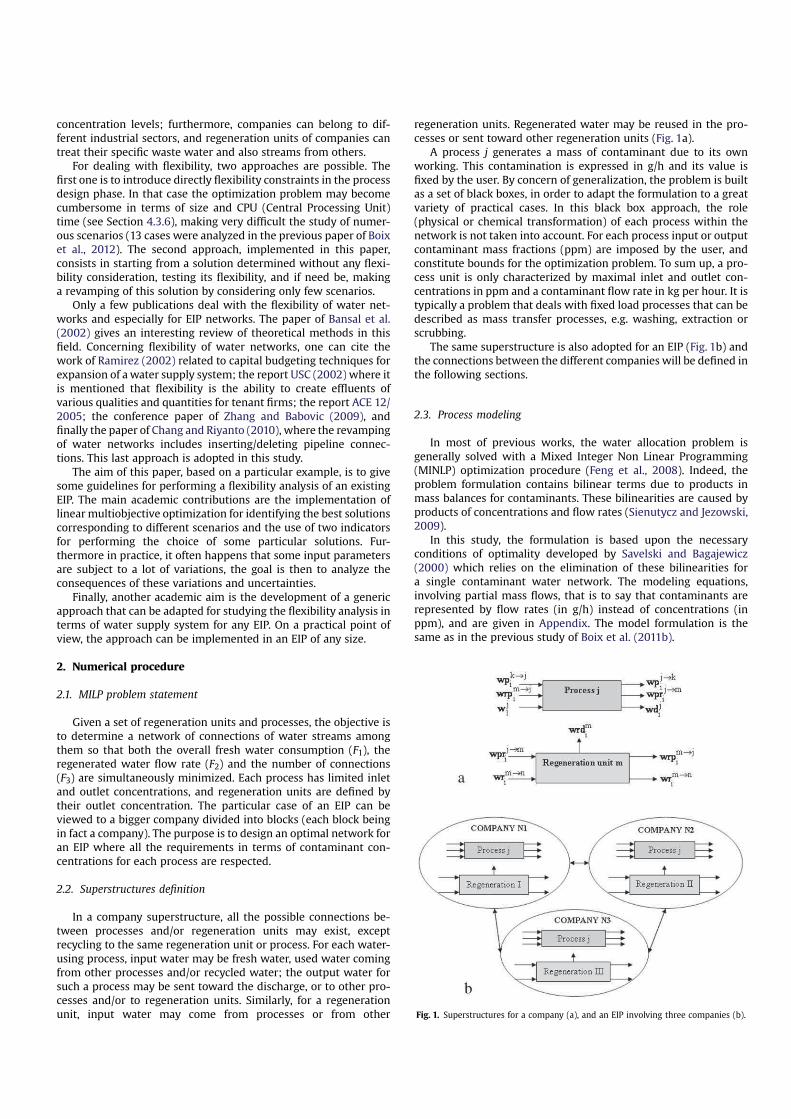
2.2. Superstructures definition
In a company superstructure, all the possible connections be-
tween processes and/or regeneration units may exist, except
recycling to the same regeneration unit or process. For each water-
using process, input water may be fresh water, used water coming
from other processes and/or recycled water; the output water for
such a process may be sent toward the discharge, or to other pro-
cesses and/or to regeneration units. Similarly, for a regeneration
unit, input water may come from processes or from other
regeneration units. Regenerated water may be reused in the pro-
cesses or sent toward other regeneration units (Fig. 1a).
A process j generates a mass of contaminant due to its own
working. This contamination is expressed in g/h and its value is
fixed by the user. By concern of generalization, the problem is built
as a set of black boxes, in order to adapt the formulation to a great
variety of practical cases. In this black box approach, the role
(physical or chemical transformation) of each process within the
network is not taken into account. For each process input or output
contaminant mass fractions (ppm) are imposed by the user, and
constitute bounds for the optimization problem. To sum up, a pro-
cess unit is only characterized by maximal inlet and outlet con-
centrations in ppm and a contaminant flow rate in kg per hour. It is
typically a problem that deals with fixed load processes that can be
described as mass transfer processes, e.g. washing, extraction or
scrubbing.
The same superstructure is also adopted for an EIP (Fig. 1b) and
the connections between the different companies will be defined in
the following sections.
2.3. Process modeling
In most of previous works, the water allocation problem is
generally solved with a Mixed Integer Non Linear Programming
(MINLP) optimization procedure (Feng et al., 2008). Indeed, the
problem formulation contains bilinear terms due to products in
mass balances for contaminants. These bilinearities are caused by
products of concentrations and flow rates (Sienutycz and Jezowski,
2009).
In this study, the formulation is based upon the necessary
conditions of optimality developed by Savelski and Bagajewicz
(2000) which relies on the elimination of these bilinearities for
a single contaminant water network. The modeling equations,
involving partial mass flows, that is to say that contaminants are
represented by flow rates (in g/h) instead of concentrations (in
ppm), and are given in Appendix. The model formulation is the
same as in the previous study of Boix et al. (2011b).
Fig. 1. Superstructures for a company (a), and an EIP involving three companies (b).
2.4. Multiobjective optimization
The main goal of multiobjective optimization is to provide good
trade-offs between conflicting objectives by using for instance the
notion of non domination (see equation (4)). Multiobjective opti-
mization makes part of our current life; for example when a cus-
tomer buys a car, he tries to reach a satisfactory compromise
between the investment cost and the operating cost.
As it involves real variables (flow rates) and binary ones (exis-
tence of connections), the problem is a mixed-integer one. By using
partial flow rates instead of concentrations and the necessary
conditions of Savelski and Bagajewicz (2000), the set of constraints
defined in Appendix is linear. The considered objectives to be
simultaneously minimized are the fresh water flow rates at the
network entrances F1, the water flow rates at inlets of regeneration
units F2. They are conflicting ones, because if the fresh water flow
rate is decreased, the regenerated water flow has to be increased.
Let us note that F1 and F2 are expressed linearly in terms of flow
rates. Insofar as it involves linear objectives submitted to a linear
set of constraints, the problem is a biobjective MILP (Mixed Integer
Linear Programming) one. Another objective is the number of
connections into the network, F3, expressed as a sum of binary
variables. F3 is deliberately formulated in terms of connections
number, because if a cost is attributed, the objective function linked
to connections does not follow a linear formulation (see Sienutycz
and Jezowski, 2009). As in practice, F3 covers a restricted range of
integer values, the biobjective problem Min(F1, F2) was solved by
considering several values of F3 as additional linear equality
constraints.
When dealing with multiobjective optimization, the classical
optimality conditions of Kuhn-Tucker developed in the mono-
bjective case do not hold, because Rn is not provided with a total
relation order, for n $ 2. The solution, generally adopted consists in
defining a set of non dominated solutions, also called a Pareto front.
A general multiobjective optimization problem is formulated as:
MinFðxÞ ¼h
f1ðxÞ; f2ðxÞ; .:; fp"
x#iT
(1)
where x ˛ X3 Rn ' Nm (2)
The subspace X is defined by a set of equalityeinequality
constraints:
X ¼%
x˛Rn ' Nm=giðxÞ ( 0; i ¼ 1 to r; hj&
x'
¼ 0;
j ¼ 1 to s; l&
i'
( x&
i'
( u&
i'( (3)
The Pareto optimal or non dominated solutions are the solutions
that cannot be improved in one objective function without dete-
riorating the performance in at least one of the other objectives.
The mathematical definition of a Pareto solution is the following:
a feasible solution x* of the multiobjective optimization problem is
non-dominated if there is no other feasible solution x such as:
fiðxÞ ( fiðx*Þci˛f1; :::; pg (4)
with at least one strict inequality. The set of non dominated solu-
tions constitute the Pareto front, i.e. the set of problem solutions
amongst which the decision maker has to perform his choice.
Several Multiple Criteria Decision Methods are available in the lit-
erature, one of the most popular one being TOPSIS (Chen et al.,
2009). TOPSIS is an evaluation method where the distance be-
tween available solutions and the ‘optimized ideal reference point’
is calculated. The optimized ideal reference point is a theoretical
point where both objectives are at their minimal values. This
program calculates this distance and ranks them by increasing or-
der of distance.
2.5. Comparison strategy
In what follows, internal connections refer to connections be-
tween processes of the same company and external connections
(between two companies) are related to connections coming from
or going toward other companies. The industrial symbiosis in the
park comes into play through these external connections. By sup-
posing constant distances between companies, it is assumed that
for each external connection, the cost for each company is divided
by two. If distances are different a convex weighted sum of the
number of external connections can be used in relation (5). For EIPs
involving an interceptor for sharing regeneration units, the con-
nections between a given company and the interceptor are con-
sidered as external connections. Thus, the Equivalent Number of
Connections (ENC) for a given company, which reflects the com-
plexity of the associated infrastructure, is given by:
ENC ¼ number or internal connectionsþ 0:5
' number of external connections (5)
The number of connections has a significant economic impact,
as it is shown in Chew et al. (2008) and Boix et al. (2012) (see
Section 4.3.2).
Another economic indicator, the Global Equivalent Cost (GEC) in
fresh water flow rate, was defined (Boix et al., 2011a). This cost is
expressed as an equivalent of fresh water flow rate in T/h. For
comparison purposes, we could use the prices of fresh water, of
regenerated water and of post-treatment in the waste, which rep-
resents the cost for treating polluted water (costs of plants, of
chemicals, manpower) before recycling it. However, these prices
are strongly linked to the country and even to regions of a given
state.
GEC ¼ F1 þ RþW (6)
where F1 is defined above, R and W are the contributions of re-
generated and waste waters, with:
R ¼ a' F2 andW ¼ b' Fw (7)
where Fw is the waste water flow rate.
Combining relations (6) and (7) leads to the following relation:
GEC ¼ F1 þ a' F2 þ b' Fw (8)
In the previous relations, a depends on the type of regeneration
unit (see Table 1) and b ¼ 5.625 according to Bagajewicz and Faria
(2009).
After the multiobjective optimization step, the different solu-
tions are discriminated by performing a Pareto front sorting on
couples (GEC, ENC) for each company, which are related to the
economic dimension of the EIP. In fact, by implementing a bio-
bjective optimization a Pareto front is obtained instead of a single
solution as in the monobjective case (with the total cost to be
Table 1
Values of a according to types of regeneration units.
Regeneration type Outlet concentration (ppm) a value
I 50 0.375
II 20 1.75
III 5 3.125
minimized for instance). Here all the results provided by the bio-
bjective optimization are presented first and a tool for decision aid
is then used for determining the set of “best” solutions. The
advantage of this method is to provide results, without any pref-
erence a priori on objectives and that can be treated with several
Multiple Choice Decision Making (MCDM) tools. Furthermore, if
a cost is considered as an objective function, the multiobjective
optimization problem cannot remain linear. It is worth noting that
the results provided by the Pareto front can be evaluated in terms of
cost in the post-optimization stage, by introducing the cost as
a supplementary item in the MCDM procedure.
3. Best EIP
3.1. Problem formulation
The example proposed by Olesen and Polley (1996), is used as
illustration purpose. The industrial pool involves three companies,
each one including five processes; the data are displayed in
Table 2.
In a preliminary study (Boix et al., 2012), the water network was
designed for each company without considering the EIP in order to
determine the best regeneration unit chosen by each company
among the three types listed in Table 3. From this multiobjective
optimization study (objectives F1, F2 and with constraint F3), the
best solution is obtained when companies A and B choose regen-
eration unit I, and company C, regeneration unit II. This solution is
given by themedian point of the Pareto front (F1, F2) for theminimal
value of F3 (reference case 0 of Table 4).
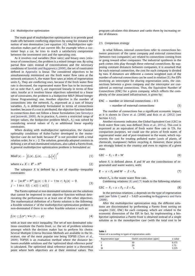
The three companies decide to pursuit an industrial symbiosis
for managing their used waters inside an EIP. The superstructure of
the EIP is shown in Fig. 2. The objective is to identify the best
strategy for each company so as to minimize the global equivalent
cost (GEC) and the number of connections in the network (ENC). For
each scenario, several situations were analyzed: different gains for
companies, restricted number of connections, and same gain for all
the companies. The major constraint is that the EIP has to be eco-
nomically profitable, that is to say, the gains for each companymust
be positive.
3.2. Problem solution
In a first step, the range of possible values for the number of
connections F3 in the EIP is defined. Then the water allocation
problem consists in solving the biobjective problem Min (F1, F2)
under the constraint F3 fixed at a given value in the previous range.
The multiobjective method based on the ε-constraint two-phase
strategy (Mavrotas, 2009), was implemented (details are given in
Boix et al., 2012). For each biobjective solution, the median point of
the Pareto front is retained if it does not involve connections with
flows lower than 2 T/h (for avoiding using very small pipes, with
diameter less than one inch). If this constraint does not hold for the
median solution, a neighboring solution is chosen on the Pareto
front.
Using this optimization strategy, the best solution among the
several scenarios was identified for the EIP. Two main scenarios
were studied: EIP with one regeneration unit per company (direct
integration) and EIP with a common regeneration unit (indirect
integration), and for each scenario several cases (restricted number
of connections, same or different gains for companies). This best
solution (case 1) corresponds to a direct integration strategy (pri-
vate regeneration units) for this particular network.
The results are displayed in Table 4, where the gains are com-
puted vs. the reference case, case 0. This case corresponds to stand-
alone companies (not included in the EIP), with private regener-
ation units (Type I for A and B, type II for C, Boix et al., 2012). In the
proposed solution, it was imposed that the three companies have
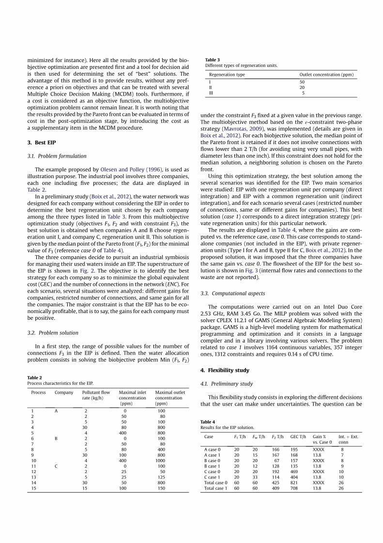
the same gain vs. case 0. The flowsheet of the EIP for the best so-
lution is shown in Fig. 3 (internal flow rates and connections to the
waste are not reported).
3.3. Computational aspects
The computations were carried out on an Intel Duo Core
2.53 GHz, RAM 3.45 Go. The MILP problem was solved with the
solver CPLEX 11.2.1 of GAMS (General Algebraic Modeling System)
package. GAMS is a high-level modeling system for mathematical
programming and optimization and it consists in a language
compiler and in a library involving various solvers. The problem
related to case 1 involves 1164 continuous variables, 357 integer
ones, 1312 constraints and requires 0.14 s of CPU time.
4. Flexibility study
4.1. Preliminary study
This flexibility study consists in exploring the different decisions
that the user can make under uncertainties. The question can be
Table 2
Process characteristics for the EIP.
Process Company Pollutant flow
rate (kg/h)
Maximal inlet
concentration
(ppm)
Maximal outlet
concentration
(ppm)
1 A 2 0 100
2 2 50 80
3 5 50 100
4 30 80 800
5 4 400 800
6 B 2 0 100
7 2 50 80
8 5 80 400
9 30 100 800
10 4 400 1000
11 C 2 0 100
12 2 25 50
13 5 25 125
14 30 50 800
15 15 100 150
Table 3
Different types of regeneration units.
Regeneration type Outlet concentration (ppm)
I 50
II 20
III 5
Table 4
Results for the EIP solution.
Case F1 T/h Fw T/h F2 T/h GEC T/h Gain %
vs. Case 0
Int. þ Ext.
conn
A case 0 20 20 166 195 XXXX 8
A case 1 20 15 167 168 13.8 7
B case 0 20 20 67 157 XXXX 8
B case 1 20 12 128 135 13.8 9
C case 0 20 20 192 469 XXXX 10
C case 1 20 33 114 404 13.8 10
Total case 0 60 60 425 821 XXXX 26
Total case 1 60 60 409 708 13.8 26
formulated as follows: “What are the consequences of some
changes in the pollutant flow rates in terms of decision making?”
According to Swaney and Grossmann (1985), one can define
a flexibility index as a measure of the maximum tolerable range of
variation in every uncertain parameter (here, the contaminant flow
rates for every process unit in the network). In the previous section,
the problem was solved for fixed values of the pollutant flow rate
for each process of each company (see Table 2). The questionwhich
arises now is to know what is the maximal increase/decrease of
pollutant flow rates, so that the existing EIP remains feasible and
profitable.
Several cases have to be studied: flow rate variations in one, two
or three companies. In the EIP, it is important to constrain each
company to have the same gain. In the following tables, notation
FA*x means that the pollutant flow rates FA of company A (third
column of Table 2) are multiplied by x, and (FA þ FB)*x means that
the pollutant flow rates FA of company A and FB of company B are
multiplied by x.
The value of x is determined by a simple dichotomy procedure.
For example, considering an increase of the flow rates in company
A, and assuming x ˛ [1, 2], if for x ¼ 2, the EIP is unfeasible or has
a gain less or equal a given threshold, x is replaced by 1.5, and so on.
The Gain After a Variation of x (GAVc) for a company c (c¼ A, B or
C) is computed according to the following expression:
GAVc ¼ ðx*GECc incase0eNewGECcÞ=ðx*GECc incase0Þ (9)
where New GECc is the GEC for a company c, computed by opti-
mizing the flow rates in the EIP (with fixed number of connections,
for example, for case 1, the value is set at 26).
Let us note that if the pollutant flow rates in a company are
multiplied by x, insofar as the outlet concentrations are fixed at
their maximal values (theorems of Savelski and Bagajewicz, 2000),
all the flows are multiplied by x. So, after an increase of x, the GEC is
also multiplied by x. It is the same case for a decrease.
For case 1, the gains of the three companies vs. the reference case
0 (GECc in case 0) is 13.8% for x ¼ 1 (see Table 4). The values of GAV
related to case 1 (best solution, one regeneration unit per company,
26 connections) are displayed in Table 5. The limit value of x, xlim,
reported in this Table, corresponds to the limit beyond which the
network becomes unfeasible for performing the polluted water
treatment.
The flexibility of company C is near zero. For an increase x
greater than 1.01, the EIP of case 1 becomes unfeasible. The EIP
network being flexible in no way, we did not pursue further this
study with an increase of the pollutant flow rates for companies
A&B, A&C, B&C, A&B&C. Indeed, the lack of flexibility comes from
the fact that company C is more demanding than the two other
ones in terms of pollutant loads to be treated.
4.2. Discussion
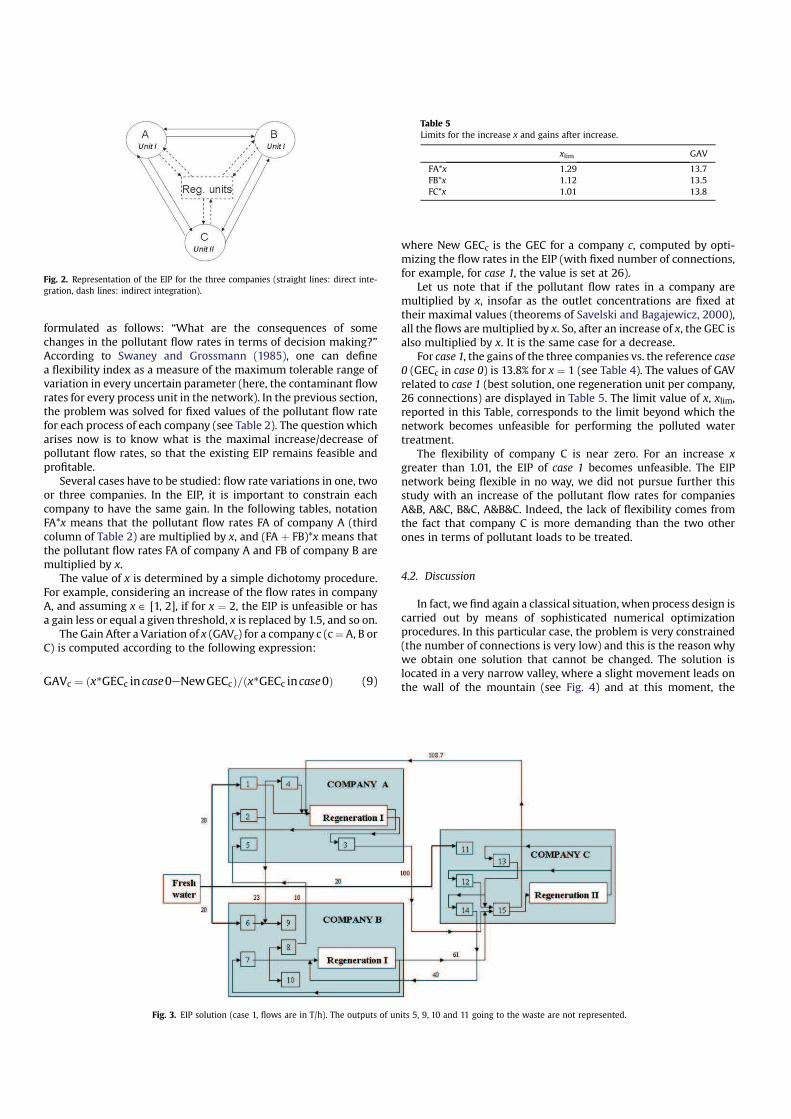
In fact, we find again a classical situation, when process design is
carried out by means of sophisticated numerical optimization
procedures. In this particular case, the problem is very constrained
(the number of connections is very low) and this is the reason why
we obtain one solution that cannot be changed. The solution is
located in a very narrow valley, where a slight movement leads on
the wall of the mountain (see Fig. 4) and at this moment, the
Fig. 3. EIP solution (case 1, flows are in T/h). The outputs of units 5, 9, 10 and 11 going to the waste are not represented.
Fig. 2. Representation of the EIP for the three companies (straight lines: direct inte-
gration, dash lines: indirect integration).
Table 5
Limits for the increase x and gains after increase.
xlim GAV
FA*x 1.29 13.7
FB*x 1.12 13.5
FC*x 1.01 13.8
problem becomes unfeasible. The best EIP identified by the bio-
bjective optimization Min (F1, F2) corresponds to the minimal value
of GEC, for the minimal value of internal and external connections
(26).
The only solution to return the proposed network flexible is to
increase the number of connections. Let us note that only internal
connections are concerned, insofar as it is assumed that each
company has always two external input and two external output
connections (see Fig. 2). However, it must be kept in mind that
connections have a cost, so the increase of the number of connec-
tions needs to remain moderate. We have limited it at 30 connec-
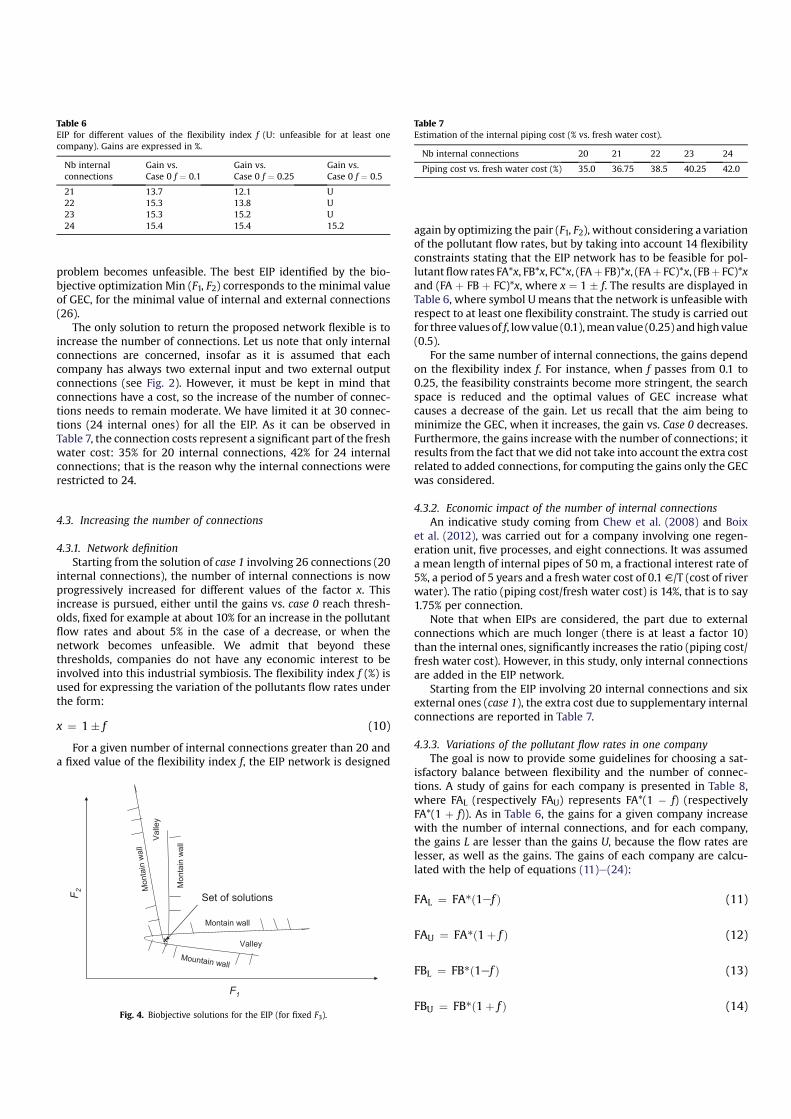
tions (24 internal ones) for all the EIP. As it can be observed in
Table 7, the connection costs represent a significant part of the fresh
water cost: 35% for 20 internal connections, 42% for 24 internal
connections; that is the reason why the internal connections were
restricted to 24.
4.3. Increasing the number of connections
4.3.1. Network definition
Starting from the solution of case 1 involving 26 connections (20
internal connections), the number of internal connections is now
progressively increased for different values of the factor x. This
increase is pursued, either until the gains vs. case 0 reach thresh-
olds, fixed for example at about 10% for an increase in the pollutant
flow rates and about 5% in the case of a decrease, or when the
network becomes unfeasible. We admit that beyond these
thresholds, companies do not have any economic interest to be
involved into this industrial symbiosis. The flexibility index f (%) is
used for expressing the variation of the pollutants flow rates under
the form:
x ¼ 1# f (10)
For a given number of internal connections greater than 20 and
a fixed value of the flexibility index f, the EIP network is designed
again by optimizing the pair (F1, F2), without considering a variation
of the pollutant flow rates, but by taking into account 14 flexibility
constraints stating that the EIP network has to be feasible for pol-
lutantflow rates FA*x, FB*x, FC*x, (FAþ FB)*x, (FAþ FC)*x, (FBþ FC)*x
and (FA þ FB þ FC)*x, where x ¼ 1 # f. The results are displayed in
Table 6, where symbol Umeans that the network is unfeasible with
respect to at least one flexibility constraint. The study is carried out
for three values of f, lowvalue (0.1),meanvalue (0.25) andhighvalue
(0.5).
For the same number of internal connections, the gains depend
on the flexibility index f. For instance, when f passes from 0.1 to
0.25, the feasibility constraints become more stringent, the search
space is reduced and the optimal values of GEC increase what
causes a decrease of the gain. Let us recall that the aim being to
minimize the GEC, when it increases, the gain vs. Case 0 decreases.
Furthermore, the gains increase with the number of connections; it
results from the fact that we did not take into account the extra cost
related to added connections, for computing the gains only the GEC
was considered.
4.3.2. Economic impact of the number of internal connections
An indicative study coming from Chew et al. (2008) and Boix
et al. (2012), was carried out for a company involving one regen-
eration unit, five processes, and eight connections. It was assumed
a mean length of internal pipes of 50 m, a fractional interest rate of
5%, a period of 5 years and a freshwater cost of 0.1V/T (cost of river
water). The ratio (piping cost/fresh water cost) is 14%, that is to say
1.75% per connection.
Note that when EIPs are considered, the part due to external
connections which are much longer (there is at least a factor 10)
than the internal ones, significantly increases the ratio (piping cost/
fresh water cost). However, in this study, only internal connections
are added in the EIP network.
Starting from the EIP involving 20 internal connections and six
external ones (case 1), the extra cost due to supplementary internal
connections are reported in Table 7.
4.3.3. Variations of the pollutant flow rates in one company
The goal is now to provide some guidelines for choosing a sat-
isfactory balance between flexibility and the number of connec-
tions. A study of gains for each company is presented in Table 8,
where FAL (respectively FAU) represents FA*(1 + f) (respectively
FA*(1 þ f)). As in Table 6, the gains for a given company increase
with the number of internal connections, and for each company,
the gains L are lesser than the gains U, because the flow rates are
lesser, as well as the gains. The gains of each company are calcu-
lated with the help of equations (11)e(24):
FAL ¼ FA*ð1ef Þ (11)
FAU ¼ FA*ð1þ f Þ (12)
FBL ¼ FB*ð1ef Þ (13)
FBU ¼ FB*ð1þ f Þ (14)
Table 6
EIP for different values of the flexibility index f (U: unfeasible for at least one
company). Gains are expressed in %.
Nb internal
connections
Gain vs.
Case 0 f ¼ 0.1
Gain vs.
Case 0 f ¼ 0.25
Gain vs.
Case 0 f ¼ 0.5
21 13.7 12.1 U
22 15.3 13.8 U
23 15.3 15.2 U
24 15.4 15.4 15.2
x
Set of solutions
Valley
Va
lley
Mountain wall
Montain wall
Monta
inw
all
Mo
nta
inw
all
F1
F2
Fig. 4. Biobjective solutions for the EIP (for fixed F3).
Table 7
Estimation of the internal piping cost (% vs. fresh water cost).
Nb internal connections 20 21 22 23 24
Piping cost vs. fresh water cost (%) 35.0 36.75 38.5 40.25 42.0
FCL ¼ FC*ð1ef Þ (15)
FCU ¼ FC*ð1þ f Þ (16)
FABL ¼ ðFAþ FBÞ*ð1ef Þ (17)
FABU ¼ ðFAþ FBÞ*ð1þ f Þ (18)
FACL ¼ ðFAþ FCÞ*ð1ef Þ (19)
FACU ¼ ðFAþ FCÞ*ð1þ f Þ (20)
FBCL ¼ ðFBþ FCÞ*ð1ef Þ (21)
FBCU ¼ ðFBþ FCÞ*ð1þ f Þ (22)
FABCL ¼ ðFAþ FBþ FCÞ*ð1ef Þ (23)
FABCU ¼ ðFAþ FBþ FCÞ*ð1þ f Þ (24)
Obviously, the mean gains decrease when the flexibility index f
increases. When passing from a low flexibility level (f ¼ 0.1) to
a mean flexibility level (f ¼ 0.25), this decrease being small, the
lower level of flexibility is not any more considered. To pursue the
flexibility study, the cases (f ¼ 0.25, number of internal
connections ¼ 23 e scenario 1) and (f ¼ 0.5, number of internal
connections ¼ 24 e scenario 2) have been retained. Let us note that
when passing to 20 internal connections as in the case 1, to 23 in
scenario 1 (respectively to 24 in scenario 2), the extra cost due to the
increase of the number of connections is estimated at 5.25%
(respectively 7%) in terms of fresh water cost (see Table 7).
4.3.4. Variations of the pollutant flow rates in two companies
If the pollutant flow rate variations are planned to occur into
two companies (AB), or (AC), or (BC), the problem is now to know if
the EIP structure identified in scenario 1 (respectively scenario 2)
remains economically profitable.
The lower and upper values for the GEC are displayed in Table 9;
they are computed according to relation (9), where the GAV is
known from Table 8. For example, New GECAL is given by
((0.75*195) e New GECAL)/(0.75*195) ¼ 0.137, that is to say, New
GECAL ¼ 126.1.
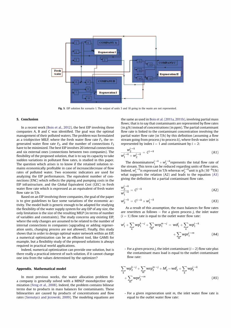
The results for the GAV are reported in Table 10. For example in
scenario 1, from Tables 4 and 9, the GAV for ABL is computed as
follows: GAVABL ¼ (0.75*(195 þ 157) + (126.1 þ 101.1))/
(0.75*(195 þ 157)) ¼ 13.9. From Table 10, the two scenarios are
economically viable. The gains in GAV and the extra cost due to the
number of connections are better for scenario 1 than for scenario 2,
but scenario 2 offers more flexibility.
4.3.5. Variations in the three companies
This is the more general case, where the economic analysis does
not allow targeting one or two particular companies. The pollutant
flow rate variations can occur in the three companies; the results
are reported in Table 11. Concerning the comparison of the two
scenarios, the conclusion is the same as in the previous case. The
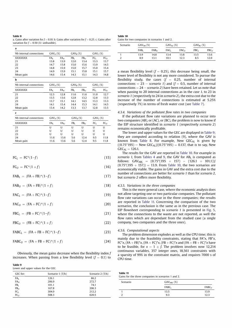
EIP flowsheet corresponding to scenario 1 is presented in Fig. 5,
where the connections to the waste are not reported, as well the
flow rates which are dependant from the studied case (a single
company, two companies and the three ones).
4.3.6. Computational aspects
The problem dimension explodes as well as the CPU time; this is
mainly due to the feasibility constraints, stating that FA*x, FB*x,
FC*x, (FAþ FB)*x, (FAþ FC)*x, (FBþ FC)*x and (FAþ FBþ FC)*x have
to be feasible, for x ¼ 1 # f. The problem involves now 12,214
continuous variables, 357 integer ones, 18,561 constraints with
a sparsity of 99% in the constraint matrix, and requires 7000 s of
CPU time.
Table 9
Lower and upper values for the GEC.
GEC for: Scenario 1 (T/h) Scenario 2 (T/h)
FAL 126.1 86.2
FAU 206.9 272.7
FBL 101.1 74.1
FBU 167.8 206.3
FCL 304.9 212.2
FCU 508.3 620.5
Table 10
Gains for two companies in scenarios 1 and 2.
Scenario GAVAB (%) GAVAC (%) GAVBC (%)
FABL FABU FACL FACU FBCL FBCU
1 13.9 14.8 13.4 13.8 13.5 13.6
2 8.9 13.1 10.1 12.3 8.5 12.0
Table 11
Gains for the three companies in scenarios 1 and 2.
Scenario GAVABC (%)
FABCL FABCU
1 13.5 13.9
2 9.3 12.3
Table 8
a. Gains after variation for f ¼ 0.10. b. Gains after variation for f ¼ 0.25. c. Gains after
variation for f ¼ 0.50 (U: unfeasible).
a
Nb internal connections GAVA (%) GAVB (%) GAVC (%)
XXXXXXX FAL FAU FBL FBU FCL FCU
21 13.8 13.9 12.0 13.4 13.3 13.7
22 14.7 15.8 15.0 15.6 13.9 14.5
23 14.8 15.9 15.0 15.7 15.0 15.4
24 14.9 15.9 15.1 15.8 15.1 15.7
Mean gain 14.6 15.4 14.3 15.1 14.3 14.8
b
Nb internal connections GAVA (%) GAVB (%) GAVC (%)
XXXXXXX FAL FAU FBL FBU FCL FCU
21 12.3 12.8 11.6 11.6 11.0 12.7
22 13.5 13.6 12.8 13.2 12.8 13.3
23 13.7 15.1 14.1 14.5 13.3 13.3
24 14.1 15.4 14.4 15.3 14.1 14.5
Mean gain 13.4 14.2 13.3 13.7 12.8 13.5
c
Nb internal connections GAVA (%) GAVB (%) GAVC (%)
XXXXXXX FAL FAU FBL FBU FCL FCU
21 U U U U U U
22 U U U U U U
23 U U U U U U
24 11.6 13.6 5.6 12.4 9.5 11.8
Mean gain 11.6 13.6 5.6 12.4 9.5 11.8
5. Conclusion
In a recent work (Boix et al., 2012), the best EIP involving three
companies A, B and C was identified. The goal was the optimal
management of their polluted waters. The problemwas formulated
as a triobjective MILP, where the fresh water flow rate F1, the re-
generated water flow rate F2, and the number of connections F3have to beminimized. The best EIP involves 20 internal connections
and six external ones (connections between two companies). The
flexibility of the proposed solution, that is to say its capacity to take
sudden variations in pollutant flow rates, is studied in this paper.
The question which arises is to know if the retained solution re-
mains economically profitable in case of increase/decrease of flow
rates of polluted water. Two economic indicators are used for
analyzing the EIP performances. The equivalent number of con-
nections (ENC) which reflects the piping and pumping costs in the
EIP infrastructure, and the Global Equivalent Cost (GEC) in fresh
water flow rate which is expressed as an equivalent of fresh water
flow rate in T/h.
Based on an EIP involving three companies, the goal of the paper
is to give guidelines to face some variations of the economic ac-
tivity. The model built is generic enough to be adapted for studying
the flexibility of the water supply system for any EIP of any size, the
only limitation is the size of the resulting MILP (in terms of number
of variables and constraints). The study concerns any existing EIP,
where the only changes are assumed to be related to the number of
internal connections in companies (upgrading or adding regener-
ation units, changing process are not allowed). Finally, this study
shows that in order to design optimal water network within an EIP,
a numerical optimization can be an efficient tool, like GAMS for
example, but a flexibility study of the proposed solutions is always
required in practical world applications.
Indeed, numerical optimization can provide one solution, but is
there really a practical interest of such solution, if it cannot change
one iota from the values determined by the optimizer?
Appendix. Mathematical model
In most previous works, the water allocation problem for
a company is generally solved with a MINLP monobjective opti-
mization (Feng et al., 2008). Indeed, the problem contains bilinear
terms due to products in mass balances for contaminants. These
bilinearities are caused by products of concentrations and flow
rates (Sienutycz and Jezowski, 2009). The modeling equations are
the same as used in Boix et al. (2011a, 2011b), involving partial mass
flows; that is to say that contaminants are represented by flow rates
(in g/h) instead of concentrations (in ppm). The partial contaminant
flow rate is linked to the contaminant concentration involving the
partial water flow rate (in T/h) by this definition (assuming a flow
stream going from process j to process k), where fresh water inlet is
represented by index i ¼ 1 and contaminant by i ¼ 2:
wj/k2
wj/k1 þwj/k
2
¼ Cj/k (A1)
The denominatorwj/k1 þwj/k
2 represents the total flow rate of
the stream. This term can be reduced regarding units of flow rates.
Indeed, wj/k1 is expressed in T/h whereas wj/k
2 unit is g/h (10+6T/h)
what supports the relation (A2) and leads to the equation (A3)
giving the definition for a partial contaminant flow rate.
wj/k2
wj/k1
¼ Cj/k (A2)
wj/k2 ¼ Cj/k 'wj/k
1 (A3)
As a result of this assumption, the mass balances for flow rates
are rewritten as follows e For a given process j, the inlet water
(i ¼ 1) flow rate is equal to the outlet water flow rate:
wj1 þ
X
k
wpk/j1 þ
X
m
wrpm/j1 ¼ wdj1 þ
X
k
wpj/k1
þX
m
wprj/m1 (A4)
- For a given process j, the inlet contaminant (i¼ 2) flow rate plus
the contaminant mass load is equal to the outlet contaminant
flow rate:
X
k
wpk/j2 þ
X
m
wrpm/j2 þMj
2 ¼wdj2 þX
k
wpj/k2
þX
m
wprj/m2 (A5)
- For a given regeneration unit m, the inlet water flow rate is
equal to the outlet water flow rate:
Fig. 5. EIP solution for scenario 1. The output of units 5 and 10 going to the waste are not represented.

X
n
wrn/m1 þ
X
j
wprj/m1 ¼ wrdm1 þ
X
j
wrpm/j1 þ
X
n
wrm/n1
(A6)
- For a given regeneration unitm, the inlet contaminant flow rate
is equal to the outlet contaminant flow rate:
X
n
wrn/m2 þ
X
j
wprj/m2 ¼ wrdm2 þ
X
j
wrpm/j2 þ
X
n
wrm/n2
(A7)
- The overall freshwater flow rate is equal to the total discharged
water flow rate:
X
m
wrdm1 þX
j
wdj1 ¼X
j
wj1 (A8)
- The total discharged contaminant flow rate is equal to the sum
of contaminant mass loads of each process j:
X
m
wrdm2 þX
j
wdj2 ¼X
j
Mj2 (A9)
Equations (A10) and (A11) are used to introduce two new no-
tations for the total inlet and outlet flow rates in a given process j.
wjiþX
k
wpk/ji
þX
m
wrpm/ji
¼ wpjin;i
(A10)
X
k
wpj/ki þ
X
m
wprj/mi þwdji ¼ wpjout;i (A11)
Given this set of mass balances equations, constraints on con-
taminant concentrations are added to the mathematical problem.
Each process is limited vs. inlet and outlet contaminant concen-
tration following these inequalities (for a process j):
wpjin;2
( Cmaxinj 'wpjin;2
(A12)
wpjout;2 ( Cmaxoutj 'wpjout;2 (A13)
In the same way, the post-regeneration concentration is fixed
and gives birth to equality (A14).
wrmout;2 ¼ Croutm 'wrmout;1 (A14)
The addition of constraint (A13) is not without repercussions
because it represents mass balances at splitters. Consequently, the
output streams of a given process must have the same pollutant
concentration and this assumption is mathematically conveyed for
the outlet of a process j as:
wpj/k2 + Cmaxoutj 'wpj/k
1 ¼ wprj/m2 + Cmaxoutj 'wprj/m
1
¼ wdj2 + Cmaxoutj 'wdj1 (A15)
In the same way, for the regeneration unit m, it comes:
wrm/n2 +Croutm 'wrm/n
1 ¼wrpm/j2 +Croutm 'wrpm/j
1 (A16)
However, these equalities hide an important condition. Indeed,
if the mass flow of water is null for one stream, this stream does not
exist, what is translated by the logic condition (A17):
if wpj/k1 ¼ 0 then wpj/k
2 ¼ 0 (A17)
It changes equation (A15) in equation (A18), if the process j does
not distribute water to another process k; it comes:
0 ¼ wprj/m2 + Cmaxoutj 'wprj/m
1 ¼ wdj2 + Cmaxoutj 'wdj1
(A18)
Thus,
wprj/m2 ¼ Cmaxoutj 'wprj/m
1 (A19)
The former demonstration changes the logic equation (A17) into
the equality (A19), and thus, implies that outlet concentrations are
equal to the maximal value Cmaxoutj for each process of the net-
work. The above problem checks all the necessary optimality con-
ditions for a single contaminant water allocation problem given by
Savelski and Bagajewicz (2000). According to this formulation, the
problem is linear. Nevertheless, in order to design the water supply
network, a binary variable is assigned to each flow, what changes
the problem into a MILP one. These variables y are added in the
program with the help of a big-U constraint as (U has to be bigger
than any water flow rate of the plant): wji ( yji ' U(A20) Now, the
problem has a mixed-integer linear form. For the case of an EIP,
these equations are the same for each company included in the
park.
The objectives functions are respectively: F1 the fresh water
consumption, F2 the regenerated water flow rate and F3 the num-
ber of connections in the network.
F1 ¼X
j
wj1 (A21)
F2 ¼X
l
0
@
X
m
wrm/l þX
j
wprj/l
1
A (A22)
F3 ¼X
k
yk (A23)
References
Advisory Council of Environment (ACE) of Hong Kong, paper 12/2005. Report on the92nd environmental impact assessment subcommittee meeting.
Alexander, B., Barton, G., Petrie, J., Romagnoli, J., 2000. Process synthesis andoptimisation tools for environmental design: methodology and structure.Comp. Chem. Eng. 24, 1195e1200.
Allenby, B., 2006. The ontologies on industrial ecology? Prog. Ind. Ecology, Int. J. 3(1e2), 28e40.
Aviso, K.B., Tan, R.R., Culaba, A.B., 2010a. Designing eco-industrial water exchangenetworks using fuzzy mathematical programming. Clean Techn. Environ. Policy12, 353e363.
Aviso, K.B., Tan, R.R., Culaba, A.B., Cruz Jr., J.B., 2010b. Bi-level fuzzy optimizationapproach for water exchange in eco-industrial parks. Process. Saf. Environ. Prot.88, 31e40.
Baas, L., Boons, F., 2004. An industrial ecology project in practice: exploring theboundaries of decision-making levels in regional industrial systems. J. Clean.Prod. 12, 1073e1085.
Bagajewicz, M., Faria, D.C., 2009. On the appropriate architecture of the water/wastewater allocation problem in process plants. Comp. Aided Chem. Eng. 26,1e20.
Bansal, V., Perkins, J.D., Pistikopoulos, E.N., 2002. Flexibility analysis and designusing a parametric framework. AIChE J. 48, 2851e2868.
Boix, M., Montastruc, L., Pibouleau, L., Azzaro-PanteL, C., Domenech, S., 2011a. Ecoindustrial parks for water and heat management. ESCAPE 21. Comp. AidedChem. Eng. 29, 1708e1712.
Boix, M., Montastruc, L., Pibouleau, L., Azzaro-PanteL, C., Domenech, S., 2011b.A multiobjective optimization framework for multicontaminant industrialwater network design. J. Environ. Manag. 92, 1802e1810.
Boix, M., Montastruc, L., Pibouleau, L., Azzaro-Pantel, C., Domenech, S., 2012. In-dustrial water management by multiobjective optimization: from individual tocollective solution through eco industrial parks. J. Clean. Prod. 22, 85e97.

Chang, C.T., Riyanto, E., 2010. Revamp heuristics for improving operational flexi-bility of water networks. Comp. Aided Chem. Eng. 28
Chen, Y., Li, K.W., Xu, H., Liu, S., 2009. A DEA-TOPSIS method for multiple criteriadecision analysis in emergency management. J. Syst. Sci. Syst. Eng. 28, 489e507.
Chertow, M.R., 2007. “Uncovering” industrial symbiosis. J. Ind. Ecol. 11, 11e30.Chew, I.M.L., Tan, R.R., Ng, D.K.S., Foo, D.C.Y., Majozi, T., Gouws, J., 2008. Synthesis of
direct and indirect interplantwaternetwork. Ind. Eng. Chem. Res. 47, 9485e9496.Chew, I.M.L., Tan, R.R., Foo, D.C.Y., Chiu, A.S.F., 2009. Game theory approach to the
analysis of interplant water integration in an eco-industrial park. J. Clean. Prod.17, 1611e1619.
Chew, I.M.L., Thillaivarrna, S.L., Tan, R.R., Foo, D.C.Y., 2011. Analysis of inter-plantwater integration with indirect integration schemes through game theoryapproach: Pareto optimal solution with interventions. Clean. Techn. Environ.Policy 13, 49e62.
Conover, W.R., 1918. Salvaging and utilizing wastes and scrap in industry. Ind. M.55.6, 449e451.
Côté, R., Cohen-Rosenthal, E., 1998. Designing eco-industrial parks: a synthesis ofsome experiences. J. Clean. Prod. 6, 181e188.
Feng, X., Bai, J., Wang, H.M., Zheng, X.S., 2008. Grass-roots design of regenerationrecycling water networks. Comp. Chem. Eng. 32, 1892e1907.
Frosh, R.A., Gallopoulos, N.E., 1989. Strategies for manufacturing. Sci. Am. 261, 144e152.
Geng, Y., Hengxin, Z., 2009. Industrial park management in the Chinese environ-ment. J. Clean. Prod. 17, 1289e1294.
Gibbs, D., Deutz, P., 2005. Implementing industrial ecology? Planning for eco-industrial parks in the USA. Geoforum 36, 452e464.
Gibbs, D., Deutz, P., 2007. Reflections on implementing industrial ecology througheco-industrial park development. J. Clean. Prod. 15, 1683e1695.
Giurco, D., Bossilkov, A., Patterson, J., Kazaglis, A., 2010. Developing industrial waterreuse synergies in Port Melbourne: cost effectiveness, barriers and opportu-nities. J. Clean. Prod. 19, 867e876.
Heeres, R.R., Vermeulen, W.J.V., de Walle, F.B., 2004. Eco-industrial parks initiativesin the USA and the Netherlands: first lessons. J. Clean. Prod. 12, 985e995.
Hoffman, C., 1971. The Industrial Ecology of Small and Intermediate-sized TechnicalCompanies: Implications forRegionalEconomicDevelopment. Reportprepared fortheEconomicDevelopmentAdministrationCOM-74-10680, TexasUniversity,USA.
Kim, S.H., Yoon, S.-G., Chae, S.H., Park, S., 2010. Economic and environmentaloptimization of a multi-site utility network for an industrial complex. J. Environ.Manag. 91, 690e705.
Liu, C., Zhang, K., Zhang, J., 2010. Sustainable utilization of regional water resources:experiences from the Hai Hua ecological industry pilot zone (HHEIPZ) project inChina. J. Clean Prod. 18, 447e453.
Lovelady, E.M., El-Halwagi, M.M., 2009. Design and integration of eco-industrialparks for managing water resources. Environ. Prog. Sustain. Energ. 28, 265e272.
Mavrotas, G., 2009. Effective implementation of the ε-constraint method in multi-objectivemathematical programming problems. Ap. Math. Comp. 213, 455e465.
Mirata, M., 2004. Experiences from early stages of a national industrial symbiosisprogramme in the UK: determinants and coordination challenges. J. Clean. Prod.12, 967e983.
Oh, D.S., Kim, K.B., Jeong, S.Y., 2005. Eco-industrial park design: a Daedeok Tech-novalley case study. Habitat. Int. 29, 269e284.
Olesen, S.G., Polley, G.T., 1996. Dealing with plant geography and piping constraintsin water network design. Trans. Chem. E. 74, 273e276.
Park, H.S., Rene, E.R., Choi, S.M., Chiu, A.S.F., 2008. Strategies for sustainable devel-opment of industrial park in Ulsan, South Koreae from spontaneous evolution tosystematic expansion of industrial symbiosis. J. Environ. Manag. 87, 1e13.
PCSD (President’s Council on Sustainable Development), 1996. Eco-efficiency TaskForce Report. D.C, USA, Washington.
Ramirez, N., 2002. Valuing flexibility in infrastructure developments. The Bogotaexpansion plan. MSc thesis. MIT.
Report University of Southern California (USC), 2002. Resource Manual on Infra-structure for Eco-industrial Development.
Roberts, B.H., 2004. The application of industrial ecology principles and planningguidelines for the development of eco-industrial parks: an Australian casestudy. J. Clean. Prod. 12, 997e1010.
Savelski, M., Bagajewicz, M., 2000. On the necessary conditions of water utilizationsystems in process plants with single contaminants. Chem. Eng. Sci. 55, 5035e5048.
Shi, H., Chertow, M., Song, Y., 2010. Developing country experience with eco-industrial parks: a case study of the Tianjin economical-technological devel-opment area in China. J. Clean. Prod. 18, 191e199.
Sienutycz, S., Jezowski, J., 2009. Energy Optimization in Process Systems e Chapter20: Approaches to Water Network Design. 613e657. Elsevier, Oxford, UK.
Simmonds, P.L., 1862. Waste Products and Undeveloped Substances. Hardwicke,London.
Swaney, R.E., Grossmann, I.E., 1985. An index for operational flexibility in chemicalprocess design. Part I. Formulation and theory. AIChE J. 31, 621e630.
Tiejun, D., 2010. Two quantitative indices for the planning and evaluation of eco-industrial parks. Res. Conserv. Recycle 54, 442e448.
Tudor, T., Adam, E., Bates, M., 2007. Drivers and limitations for the successfuldevelopment and functioning of EIPs (eco-industrial parks): a literature review.Ecol. Econ. 61, 199e207.
Van Beers, D., Corder, G., Bossilkov, A., Van Berkel, R., 2007. Industrial symbiosis inthe Australian minerals industry: the cases of Kwinana and Gladstone. J. Ind.Ecol. 11, 55e72.
Van Berkel, R., 2007. Cleaner production and eco-efficiency initiatives in WesternAustralia 1996e2004. J. Clean. Prod. 15, 741e755.
Van Leeuwen, M.G., Vermeulen, W.J.V., Glasbergen, P., 2003. Planning eco-industrialparks: an analysis of Dutch planning methods. Bus. Strat. Environ. 12, 147e162.
Veiga, E., Bechara, L., Magrini, A., 2009. Eco-industrial park development in Rio deJaneiro, Brazil: a tool for sustainable development. J. Clean. Prod. 17, 653e661.
Watanabe, C., 1972. Industrial-Ecology: Introduction of Ecology into IndustrialPolicy. Ministry of International Trade and Industry (MITI), Tokyo.
Zhang, S., Babovic, V., 2009. Architecturing water supply system. A perspective fromvalue of the flexibility. In: Second International Symposium on EngineeringSystems. MIT, June, pp. 15e17.
Zhu, L., Zhou, J., Cui, Z., Liu, L., 2010. A method for controlling enterprises access toan eco-industrial park. Sci. Total Environ. 408, 4817e4825.