The University of MaineDigitalCommons@UMaine

Electronic Theses and Dissertations Fogler Library

2003

On the Generation and Detection of UltrasonicPlate Waves in Microporous Polymeric MaterialLin Lin

Follow this and additional works at: http://digitalcommons.library.umaine.edu/etd

Part of the Mechanical Engineering Commons

This Open-Access Thesis is brought to you for free and open access by DigitalCommons@UMaine. It has been accepted for inclusion in ElectronicTheses and Dissertations by an authorized administrator of DigitalCommons@UMaine.

Recommended CitationLin, Lin, "On the Generation and Detection of Ultrasonic Plate Waves in Microporous Polymeric Material" (2003). Electronic Thesesand Dissertations. 292.http://digitalcommons.library.umaine.edu/etd/292

ON THE GENERATION AND DETECTION OF

ULTRASONIC PLATE WAVES IN MICROPOROUS

POLYMERIC MATERIAL

BY

Lin Lin

B.S. Beijing University of Technology (Beijing Polytechnic University), 1994

A THESIS

Submitted in Partial Fulfillment of the

Requirements for the Degree of

Master of Science

(in Mechanical Engineering)

The Graduate School

The University of Maine

August, 2003

Advisory Committee:

Michael Peterson, Associate Professor of Mechanical Engineering, Advisor

Donald Grant, R.C. Hill Professor and Chairman of Mechanical Engineering

Eric Landis, Associate Professor of Civil Engineering

ON THE GENERATION AND DETECTION OF

ULTRASONIC PLATE WAVES IN MICROPOROUS

POLYMERIC MATERIAL

By Lin Lin

Thesis Advisor: Dr. Michael Peterson

An Abstract of the Thesis Presented in Partial Fulfillment of the Requirements for the

Degree of Master of Science (in Mechanical Engineering)

August, 2003

Membranes are among the most important engineering components in use in

many process industries. Examples of uses for membranes include water purification,

industrial effluent treatment, recovery of volatile organic compounds, protein recovery,

bio-separations and many others. Polymeric membranes are the most commonly used

membranes. Membranes act as a barrier through which fluids and solutes are selectively

transported.

Quality assurance is a critical aspect of membrane module fabrication. In other

materials, ultrasound has been widely used for materials characterization as well as flaw

detection. Recently ultrasonic techniques have been used to detect the presence of

defects in membranes. This thesis describes the use of guided waves in membrane

applications to improve the ability to inspect large areas of membranes. Plate waves also

have the potential to provide additional information in asymmetric membranes.

The present effort focuses on developing techniques that make it possible to test

microporous membranes using low frequency ultrasonic guided waves. The sensitivity of

the material attenuation in polyvinylidene fluoride (PVDF) membrane material with

frequency was investigated. The attenuation of the PVDF membrane increases with

frequency, and does not appear linear. There is at least one inflection point occurs in the

range considered. These measurements were verified using single frequency method.

For these measurements the propagation distance and inspection area of a plate wave at

different frequencies in porous PVDF membrane were estimated. The inspection ranged

from 2.01cm2 at 2.25MHz to 7.69mm2 at 30MHz. The dispersion curve for the first mode

was obtained using experimental data, and the single mode generated in the plate was

shown to be dispersive.

ACKNOWLEDGEMENTS

I would first like to express my deep sense of gratitude towards my advisor

Professor Michael "Mick" Peterson for being an outstanding advisor. This work would

not have been possible without the constant encouragement and help from Mick.

I am grateful to Professor Donald Grant and Professor Eric Landis for taking part

in my thesis committee, and for providing me with valuable suggestion and guidance.

I would also like to thank Dr. Anthony DiLeo at Millipore Corporation for his

help in providing me with membrane samples, and valuable suggestion from an industrial

perspective.

I wish to thank Jeremy Winn for helping me with the experimental setups for this

work. I would like to thank Anthony Puckett for his help in getting me started with the

ultrasonic techniques, and many fruitful discussions with him. I would also like to thank

all the members of Mick's research group for the help, suggestions, encouragements, and

of course the friendship.

My greatest thanks go to my husband, Wenjin, and my parents for the love,

support, and encouragement.

TABLE OF CONTENTS

. . .......................................................................................... ACKNOWLEDGEMENTS i i

............................................................................................................. LIST OF TABLES vi

. . .......................................................................................................... LIST OF FIGURES vii

Chapter

...................................................................................................... . 1 INTRODUCTION 1

2 . BACKGROUND ........................................................................................................ 5

...................................................................................... 2.1 Microporous membrane 5

.......................................................................... 2.1.1 Polymers membrane types 5

............................. 2.1.2 Microporous polyvinyl de-fluoride (PVDF) membrane 6

2.1.3 Membrane defects ....................................................................................... 7

2.1.4 Membrane characterization techniques .................................................. 7

2.2 Ultrasonic waves in porous materials ................................................................. 9

2.2.1 Types of waves in porous materials ............................................................ 9

................................................................. 2.2.1.1 Fast compressional waves 10

2.2.1.2 Slow compressional waves ............................................................... 10

2.2.1.3 Transverse (shear or rotational) waves ........................................ 11

2.2.1.4 Velocities of the waves propagation in porous materials ................. 11

2.2.2 Plate waves (Lamb waves) ........................................................................ 13

2.2.2.1 Modes ................................................................................................ 14

2.2.2.2 Partial wave analysis .................................................................. 15

2.2.2.3 Phase and group velocity .................................................................. 16

iii

............................................................................... 2.2.2.4 Dispersion curve 19

................................................................. 2.2.2.5 Generation of plate waves 20

..................... 2.2.2.6 Plate wave propagation in a fluid-loaded porous plate 22

............................................. 2.3 Attenuation of the ultrasound in porous polymer 25

.............................................................................. 2.4 Ultrasonic testing technique 27

......................................................................................... 3 . LITERATURE REVIEW 29

............................................................................... Membrane characterization 29

............................................................................... Ultrasonic characterization 29

....................................... Application of ultrasonic testing to porous materials 31

Biot's theory ...................................................................................................... 33

Plate wave (Lamb wave) ................................................................................... 36

Water loading influence on guided waves ........................................................ 38

........................................................................................................... Summary 39

.......................................................................................... . 4 SIGNAL PROCESSING 41

....... 4.1 Attenuation measurement using deconvolution and Pseudo-Wiener filter 41

................................................. 4.2 Velocity measurement using cross-correlation 46

4.3 Dispersion curve by 2D Fourier transform and short time Fourier

transform (STFT) .............................................................................................. 47

4.3.1 2D Fourier transform ................................................................................ 47

4.3.2 Time frequency analysis - short time Fourier transform .......................... 48

................................................................................... 5 . EXPERIMENTAL SYSTEM 52

............................................................................................... 5.1 Materials sample 52

5.2 Wetting the membranes .................................................................................... 52

5.3 Experimental setup and data acquisition ........................................................... 54

............................ 5.3.1 Attenuation measurement with broadband transducers 54

....................... 5.3.2 Attenuation curve calibrated with single frequency signal 57

5.3.3 Plate wave generation ............................................................................... 58

.................... 5.3.4 Propagation distance of the plate wave in PVDF membrane 60

............................................................................... 6 . RESULTS AND DISCUSSION 62

6.1 Normal incidence attenuation vs . frequency ..................................................... 62

6.2 Generation of plate wave propagating in the PVDF membrane ....................... 65

6.3 Estimated propagation distance of plate waves at different frequencies in

porous PVDF membrane ................................................................................... 67

6.4 Dispersion curve ............................................................................................... 73

6.5 Discussion: Expected area of membrane to be inspected with plate

waves ................................................................................................................. 75

7 . CONCLUSIONS AND FUTURE WORK ............................................................... 78

REFERENCES ................................................................................................................. 80

APPENDICES .................................................................................................................. 84

Appendix A: Solution of the Rayleigh-Lamb frequency equations by the potential

method for fully dense plates ................................................................. 85

Appendix B: Partial wave analysis for liquid loaded dense plates .............................. 87

Appendix C: Partial wave analysis for fluid-saturated porous cylinder ...................... 90

BIOGRAPHY OF THE AUTHOR ................................................................................... 94

LIST OF TABLES

Table 1 . List of the transducers used in attenuation measurement .................................. 56

Table 2 . Distances of the plate waves propagating at different frequencies .................... 70

Table 3 . Estimated area of PVDF membrane to be inspected with plate waves .............. 77

LIST OF FIGURES

Figure 1 . Microporous membrane ...................................................................................... 6

........................................... Figure 2 . Symmetric (a) and Antisymmetric (b) plate wave 14

.................................................................... Figure 3 . Coordinate system for a free plate 14

....................................... Figure 4 . Oblique incidence for the generation of plate waves 20

.................................. Figure 5 . Transducers on the (a) same side and (b) opposite sides 21

......................... Figure 6 . Comb transducer technique for the generation of plate waves 21

Figure 7 . Coordinate system for a fluid-loaded plate ....................................................... 22

Figure 8 . Immersion-testing geometry for determining diffraction correction

integrals based on plate front- and back-surface reflections from a solid ........ 41

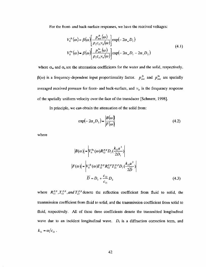
.................................... Figure 9 . Immersion-testing geometry for through transmission 43

Figure 10 . Graphical representation of the 2D Fourier Transform .................................. 48

Figure 11 . Example of effect of window length .............................................................. 50

Figure 12 . Signal segment without overlap ..................................................................... 5 1

Figure 13 . Signal segments with L overlap ...................................................................... 51

Figure 14 . Schematic representation of the wetting system ............................................. 52

Figure 15 . Effect of immersion time . a ... 5 hours; b ... 24 hours; c ... 48 hours .......... 53

Figure 16 . Schematic representation of the immersion system for the attenuation

measurement ................................................................................................... 54

Figure 17 . The frame to secure the membrane sample .................................................... 55

Figure 18 . Schematic representation of the attenuation measurement with single

frequency ......................................................................................................... 57

vii

..................... Figure 19 . Schematic representation of the system generating plate wave 59

..................... Figure 20 . Schematic drawing for the propagating distance measurement 60

........................................ Figure 21 . Normal incidence attenuation factor vs . frequency 62

..... Figure 22 . Attenuation by deconvolution as well as single frequencies experiments 64

Figure 23 . Different path of the signal ............................................................................. 66

...................................................................................... Figure 24 . Signal of plate waves 66

Figure 25 . Signals from the plate wave set.up . (a) water signal; (b) with

............................................. membrane; (c) rubber between the transducers 67

Figure 26 . Amplitudes of the plate wave propagating through membrane

at 2.25MHz frequency ..................................................................................... 68

Figure 27 . Amplitudes of the plate waves at 2.25MHz ................................................... 71

Figure 28 . Amplitudes change of the ultrasonic signal .................................................... 72

Figure 29 . Spectrogram of the plate wave using 2.25MHz transducers .......................... 73

Figure 30 . Spectrogram of (a) plate wave and (b) water signal ....................................... 74

Figure 31 . Graphical representation of beam parameters ................................................ 75

viii

Since the early 1960s, synthetic membranes have been used successfully in a wide

variety of large-scale industrial applications. Their modular nature, high selectivity, and

energy efficiency make membranes an attractive alternative to other traditional separation

processes. Membranes are among the most important engineering components in use in

many process industries, and each year more uses for membrane technologies are found.

Examples of uses for membranes include water purification, industrial effluent treatment,

recovery of volatile organic compounds, protein recovery, bio-separations and many

others [Scott 19951. Polymeric membranes are the most commonly used membranes.

Membranes act as a barrier through which fluids and solutes are selectively

transported [Mohr et a1 19891. Quality assurance is a critical aspect of membrane module

fabrication. The presence of defects in membrane structure such as pinholes and

macrovides compromise the integrity and performance of the membranes. In some

applications such as bio-pharmaceuticals these may have significant cost and efficiency

implications. Therefore, nondestructive test (NDT) techniques need to be improved for

the characterization of membranes during the fabrication process as well as during

module operation.

Current characterization techniques available for the analysis of membrane pore-

structure include scanning electron microscopy (SEM), gas permeation, and mercury

intrusion [Matsuura 19941. But, these other methods are limited by resolution, time and

cost concerns. In addition none of these techniques are applicable for on-line monitoring

with liquid separation. Recent research has demonstrated the potential of ultrasonic

techniques for the real-time nondestructive characterization of membranes. Ultrasonic

methods are attractive since they are well suited to liquid immersed membranes unlike

optical or electrical-magnetic methods. Successful application of ultrasonic techniques

has been reported for a wide range of applications including membrane formation,

compaction, and fouling [Ramaswany, 20021.

Ultrasound has been widely used for the materials characterization as well as flaw

detection [Krautkramer, 19831. Ultrasonic waves are mechanical vibrations that

propagate in an elastic medium. The characteristics of the ultrasonic waves depend on

the medium through which the waves travel. The ultrasonic properties of polymers are

influenced strongly by their molecular structure. In particular, the degree of cross-linking

and degree of crystallinity of the polymer will influence the viscoelastic and elastic

properties. Therefore the measurement of such properties is useful for the further

understanding of polymer membranes. Another important structural characterization of

membrane is the colloidal of the membrane, which governs the statistics of pores, such as

pore size, pore size distribution, pore density and void volume [Khulbe and Matsuura,

20001. Microporous membranes are typically about 70% porous; therefore, ultrasound

would be particularly well suited to characterizing membranes if the pore characteristics

of these materials could be understood. Biot's [I9561 theory for the propagation of

elastic waves through a fluid-saturated porous medium was originally developed for low

frequencies. The low frequency assumption is consistent with standard ultrasonic

frequencies in microporous membranes. It is in theory possible to relate the measured

characteristics of the ultrasonic waves to membrane characteristics of interest as several

investigators have shown [Corsaro and Sperling, 1990; Ramaswamy 20021. Attenuation

(the change of amplitude) and velocity are the two most common measurements used to

characterize any elastic medium, and are associated with each type of waves. These

characteristics of the ultrasonic waves can also be used to detect the presence of defects

in membranes. In particular, attenuation of the ultrasonic wave is due to scattering from

pores as well as due to damping in materials. Material damping is related to the

dissipation of energy during the dynamic viscous portion of deformation, and the

attenuation caused by damping is often observed to increase linearly with frequency in a

polymeric solid [Corsaro and Sperling, 19901. Pores in the membrane also act as scatters,

which cause attenuation. This scattering portion of the attenuation depends on the size of

the scatters and the frequency of the ultrasonic wave. Therefore it can provide

information about the size of the scatters. As another important acoustic measurement,

the velocity of the ultrasonic waves in porous membrane is a function of the overall

porosity of the membrane [Ramaswamy 20021.

There are different ways in which ultrasonic waves can be employed to

characterize and identify defects. A confluence of technologies has contributed to an

increase in the characterization of plate-like structures using structure-borne, or guided

waves [Chimenti, 19971. It has been well known for a long time that guided waves are

more suitable to evaluate a thin plate than the conventional bulk waves. Plate (Lamb)

waves are guided waves propagating in a plate. Numerous studies and reviews of the

characterization of plate waves have been written [Redwood, 1960; Rose, 1999;

Chimenti, 19971. Compared to the traditional bulk waves, the advantage of ultrasonic

testing with plate waves in the membrane application of interest is the capability of long

distance inspections. If the membrane is not a perfectly elastic material, attenuation due

to material dissipation exists, but the attenuation due to beam spreading is reduced by

using plate waves and it is possible to inspect a large area of a thin structure with a single

beam. Therefore, plate waves travel long distances with less attenuation than a

longitudinal wave in the membrane or other structure.

In ultrasonic guided waves, there are numerous possible modes that may

propagate in a plate. Wave velocity varies not only by the properties of the medium, but

also by the frequency, the thickness of plate, and wave mode, which is generated [Rose,

19991. At a given frequency and plate thickness, several modes may propagate with

different velocities. At a given phase velocity and plate thickness, several modes can be

excited with different frequencies. The group velocity, which is the speed of wave

energy propagating, is different from the phase velocity because of the variation in phase

velocity with frequency or the dispersion. Therefore, the dispersion characteristics of a

plate should be understood for an appropriate application of guided waves.

Thesis statement: The present effort focuses on the development of a technique

for microporous membrane characterization and testing using ultrasonic guided waves in

the low frequency range.

The variation of the attenuation of a normal incidence plane wave with frequency

will be investigated in order to understand the membrane related attenuation.

The propagation distance and area a plate wave can inspect at different

frequencies in porous PVDF membrane will be estimated.

The dispersion curve, which shows the relationship between phase velocity and

wavelength of PVDF membranes, will be discussed using experimental data for

the configuration considered.

BACKGROUND

2.1 Microporous membrane

Membranes can be used to satisfy many of the separation requirements in the

process industries. These separations can be put into two general areas: where materials

are present as a number of phases, and where species are dissolved in a single-phase

[Scott 19951. A membrane is a permeable or semi-permeable phase, polymer, inorganic

or metal, which restricts the motion of certain species. The membrane, or barrier,

controls the relative rates of transport of various species through the barrier and thus, as

with all separations, gives one product depleted in certain components and a second

product concentrated in these components. Membranes can be fabricated from a wide

variety of organic (e.g. polymers, liquids) or inorganic (e.g. carbons, zeolites, metals etc)

materials. Currently, the majority of commercial membranes are made from polymers.

2.1 .I Polymers membrane types

A membrane either has a symmetric or an asymmetric structure. Symmetric

membranes have a uniform structure throughout the entire membrane thickness, whereas

asymmetric membranes have a pore-size gradient across the cross-section of the

membrane. The gradient may or may not be uniform throughout the cross-section. The

separation properties of symmetric membranes are determined by their entire structure.

Asymmetric membranes demonstrate separation properties that are determined primarily

by the densest region on one face of the membrane. There are two kinds of symmetric

membranes: porous symmetric membranes, and dense symmetric membranes. Because

of the commercial importance of membranes, a number of monographs have been written

on the topic such as the one by Pinnan and Freeman [2000].

2.1.2 Microporous polyvinyl de-fluoride (PVDF) membrane

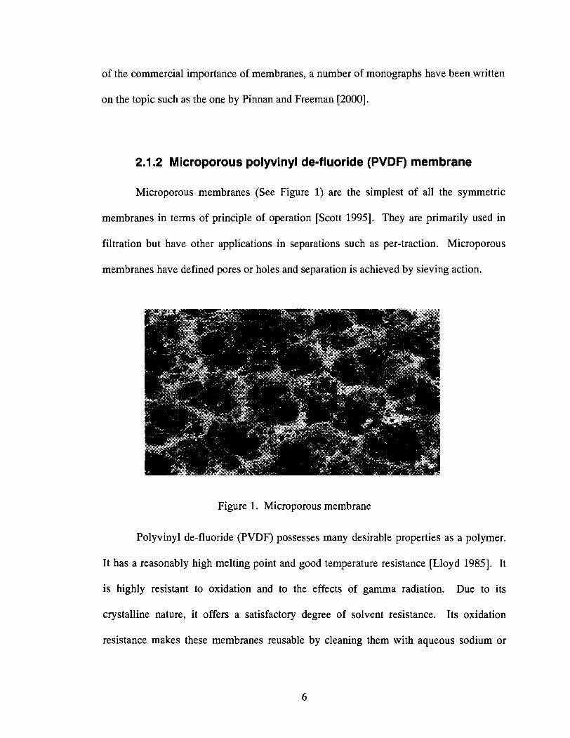
Microporous membranes (See Figure 1) are the simplest of all the symmetric

membranes in terms of principle of operation [Scott 19951. They are primarily used in

filtration but have other applications in separations such as per-traction. Microporous

membranes have defined pores or holes and separation is achieved by sieving action.

Figure 1. Microporous membrane

Polyvinyl de-fluoride (PVDF) possesses many desirable properties as a polymer.

It has a reasonably high melting point and good temperature resistance [Lloyd 19851. It

is highly resistant to oxidation and to the effects of gamma radiation. Due to its

crystalline nature, it offers a satisfactory degree of solvent resistance. Its oxidation

resistance makes these membranes reusable by cleaning them with aqueous sodium or

calcium hypochlorite or hydrogen peroxide. Also, PVDF membranes typically possess

superior ageing resistance as well as good resistance to abrasion. For these reasons, it is

desirable to have microporous PVDF membranes, which also possess suitable properties

for filtration application [Lloyd 19851.

2.1.3 Membrane defects

There are two kinds of defects present in membranes: defects caused by the

external forces during the module operation; and defects from manufacturing. Two of

the most common defects in microporous membranes are pinholes and macro-voids

[Ramaswamy 20021. Pinholes generally extend throughout the cross section of the

membrane, and are open at both surfaces. Normally the pinhole results from trapped gas

in the casting solution that escapes during membrane formation [Pinnan and Freeman

20001. The size of pinhole defects generally ranges from 100 - 1000 micron. Macro-

voids are another type of membrane defect that are often observed in membranes

manufactured using phase inversion processes. They are oversized "pores" usually

ranging from 30 - 100 microns [Ramaswamy 20021. The defects caused by external

forces varies depending on the source, thus the defects can be in any shape and size.

2.1.4 Membrane characterization techniques

Membrane characterization is a critical part of the overall membrane fabrication

process. Several techniques are available for the characterization of microporous

membrane pore structure. Scanning electron microscopy (SEM) is the most commonly

used technique. In SEM, a membrane is bombarded with a beam of electrons. These

electrons cause the sample to release secondary electrons, which are then detected, such

that an image of the impinged surface is formed. This method provides an overall view

of the membrane structure, but the sample preparation (including the freeze fracturing to

expose the cross-section and coating with a conductive metal) may change the actual

structure of the membrane. Atomic force microscopy (AMF) is a technique used to

characterize the surface of microporous membranes. AFM uses a sharp tip line-scanned

across the membrane surface with a constant force. The force between the atoms of the

probe tip and the membrane surface is measured, which therefore can be related to the

structure of the membrane surface. However, the high forces in this technique may

damage the porous structure. Bubble point method measures the pressure required to

force a gas through a liquid-filled membrane, and been used to characterize the maximum

pore size of a given liquid filled membrane. Mercury intrusion method forces mercury

into a dry membrane to get the relationship between the pressure and the volume of

mercury. Gas permeation can characterize only the active pores in the membrane and not

the dead-end pores. All of these techniques have their own advantages, but at the present

time they are limited by expensive equipment; suffer from inaccuracies due to the

process; or the possibility of damaging the porous structure [Ramaswamy, 20021.

A key advantage offered by ultrasonics is the ability for non-invasive, real-time

characterization of processes and product quality. Pioneering research showed the

application of ultrasonic for the real-time characterization of membrane formation as well

as membrane performance [Kools et al, 1998; Peterson et al, 1998; Maria1 et al, 1999;

Maria1 et al, 2000; Ramaswamy, 20021. In addition a significant area of literature

concerns waves in porous media [Mavko et al, 1998; Jones, 20011. Biot [I9561

developed perhaps the most important phenomenological model for understanding wave

propagation in fluid-saturated porous media. Based on this theory, ultrasonic waves in

porous media can be effectively exploited to measure a broad range of material properties

in porous material. These measurements include permeability of the porous frame, which

describes the overall structure as well as tortuosity [Berryman, 1981; Johnson et al, 1987;

Johnson et al, 19941.

2.2 Ultrasonic waves in porous materials

On the basis of the mode of the particle displacement, ultrasonic waves are

classified as longitudinal (dilatational) waves, transverse (shear or rotational) waves that

propagate in unbounded media, or surface waves and plate (Lamb) waves that propagate

in a half space and a layer respectively. A number of studies have attempted to model the

propagation of ultrasonic waves through porous materials, and the theory developed by

Biot is probably the most significant [Ramaswamy, 20021. For porous materials two

separate longitudinal waves propagate as well as a shear wave in an unbounded media.

2.2.1 Types of waves in porous materials

Biot [I9561 developed theoretical equations for the propagation of elastic waves

in fluid-saturated porous materials. His study predicted the existence of one shear wave

and two longitudinal waves, which were denoted as waves of the first and second kind.

The first and second dilatational waves are also known as the fast (type one) and slow

(type two) compressional waves respectively with reference to their velocity. These

waves have been shown to exist experimentally [Plona, 19801.

2.2.1 . I Fast compressional waves

The fast compressional wave usually has the higher phase velocity and typically

has lower attenuation. It deforms both the solid and fluid constituents by approximately

the same amount, and the deformations are approximately in phase [Hickey and Sabatier,

19971. The fast wave is characterized by the simultaneous compression of the pore fluid

and matrix material. It is found that the fast compressional wave velocity increases with

decreasing porosity [Plona, 19801. The dispersion due to porosity is negligible with a

phase velocity increasing or decreasing with frequency depending on the mechanical

parameters. In cases close to the dynamic compatibility condition, the dispersion and

attenuation of the fast wave tend to vanish. The attenuation of this wave may therefore

vary widely for materials of similar composition [Biot, 19561.

2.2.1.2 Slow compressional waves

The slow compressional wave has a lower phase velocity and generally larger

attenuation. Both the phase velocity and the attenuation are strongly frequency

dependent for the slow wave. The deformation associated with the slow wave consists

of primarily fluid component deformation and a very small deformation of the solid

component. The deformation of the fluid and solid components is almost 180' out of

phase [Hickey and Sabatier, 19971. Numerous attempts have been made in the

laboratory to detect this highly attenuated wave. This is due to the fact that the slow

compressional wave is characterized by the out of phase movement of the pore fluid and

the matrix materials, and offers a unique opportunity to study material properties such as

permeability and tortuosity. In contrast with the fast compressional wave, the velocity of

slow compressional wave decreases with decreasing porosity [Plona, 19801.

2.2.1.3 Transverse (shear or rotational) waves

For a transverse wave, the particle displacement at each point in a material is

perpendicular to the direction of wave propagation. Water and air do not support

transverse waves because the forces of attraction between molecules are so small that

shear waves cannot be transmitted. The same is true of any liquid other than water,

unless it is particularly viscous or is present as a very thin layer [Boyer et al, 19761. The

velocity of the transverse wave is about 50% of the longitudinal wave velocity for the

same material. For the fluid-saturated porous solid, it is found that the phase velocity of

the transverse waves increase slightly with frequency. The attenuation coefficient for

transverse waves can differ significantly from the coefficient for compressional waves in

the same material, so that separate calibration experiments must also be performed for

transverse waves [Schmerr, 19981. The speed of the transverse wave also changes with

the porosity. Plona [I9801 indicated that as the porosity decreases, the speed of the

transverse wave would increase.

2.2.1.4 Velocities of the waves propagation in porous materials

To model the propagation of ultrasonic waves through porous materials, Biot

[I9561 developed a phenomenological model of wave propagation in fluid-saturated

porous media. For a solid unbounded medium, two types of waves exist: longitudinal

waves, and transverse waves. Biot7s study predicted the existence of two longitudinal

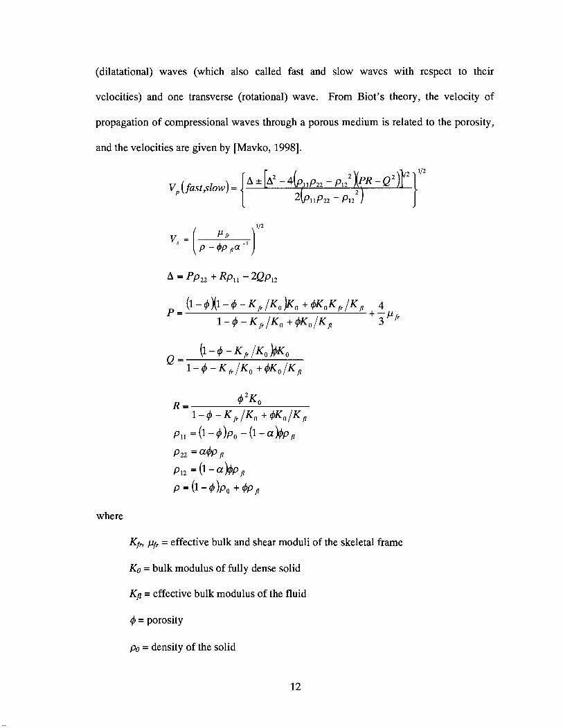
(dilatational) waves (which also called fast and slow waves with respect to their

velocities) and one transverse (rotational) wave. From Biot's theory, the velocity of

propagation of compressional waves through a porous medium is related to the porosity,

and the velocities are given by [Mavko, 19981.

where

Kfi, = effective bulk and shear moduli of the skeletal frame

KO = bulk modulus of fully dense solid

Kfl = effective bulk modulus of the fluid

+ = porosity

po = density of the solid

= density of the fluid

a = tortuosity parameter, always greater than 1

The tortuosity (also called structure factor) is a purely geometrical factor which is

dependent on the solid and liquid densities. According to Mavko et a1 [1998], Berryman

obtained the relation:

a = 1 - r(1- 114)

where, r equals to 112 for spheres, and lies between 0 and 1 for other ellipsoids. For

uniform cylindrical pores with axes parallel to the pore pressure gradient, a = 1 (which is

the smallest value for a), whereas for a random system of pores with all possible

orientations a = 3 [Stoll, 1977; Mavko et al, 19981.

These equations were derived based on the assumptions that the wavelength is

much larger than the pore scale, and the solid matrix is isotropic. These are reasonable

assumptions when normal ultrasonic frequencies are used with microporous membranes.

2.2.2 Plate waves (Lamb waves)

A plate wave is guided between two parallel free surfaces, and is generally

considered to propagate only in a solid that is several wavelengths thick. However, it can

be shown that infinitesimally thin and unbounded solids are limit cases for plate waves

[Redwood, 19601. A plate wave is the wave of plane strain that occurs in a free plate.

The traction forces must vanish on the upper and lower surface of the plate [Rose, 19991.

Apart from the material characteristics, the propagation of plate waves also depends on

the thickness of the plate, or, correspondingly, the frequency of the waves [Krautkramer,

19831.

2.2.2.1 Modes

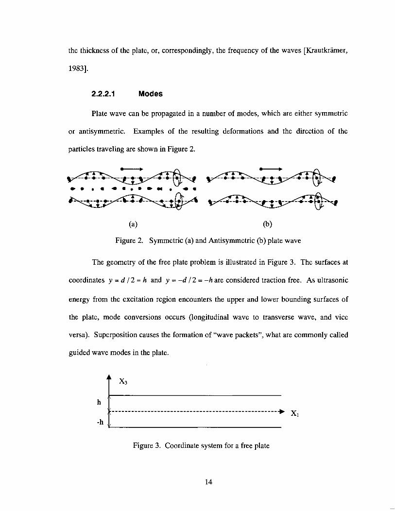
Plate wave can be propagated in a number of modes, which are either symmetric

or antisymmetric. Examples of the resulting deformations and the direction of the

particles traveling are shown in Figure 2.

(a) (b)

Figure 2. Symmetric (a) and Antisymmetric @) plate wave

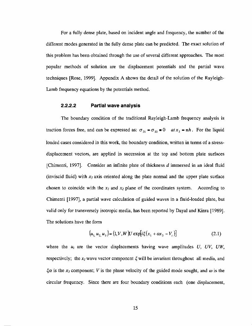
The geometry of the free plate problem is illustrated in Figure 3. The surfaces at

coordinates y = d I 2 = h and y = -d 12 = -h are considered traction free. As ultrasonic

energy from the excitation region encounters the upper and lower bounding surfaces of

the plate, mode conversions occurs (longitudinal wave to transverse wave, and vice

versa). Superposition causes the formation of "wave packets", what are commonly called

guided wave modes in the plate.

Figure 3. Coordinate system for a free plate

For a fully dense plate, based on incident angle and frequency, the number of the

different modes generated in the fully dense plate can be predicted. The exact solution of

this problem has been obtained through the use of several different approaches. The most

popular methods of solution are the displacement potentials and the partial wave

techniques [Rose, 19991. Appendix A shows the detail of the solution of the Rayleigh-

Lamb frequency equations by the potentials method.

2.2.2.2 Partial wave analysis

The boundary condition of the traditional Rayleigh-Lamb frequency analysis is

traction forces free, and can be expressed as: a,, = a,, = 0 at x, = kh . For the liquid

loaded cases considered in this work, the boundary condition, written in terms of a stress-

displacement vectors, are applied in succession at the top and bottom plate surfaces

[Chimenti, 19971. Consider an infinite plate of thickness d immersed in an ideal fluid

(inviscid fluid) with x3 axis oriented along the plate normal and the upper plate surface

chosen to coincide with the xl and xz plane of the coordinates system. According to

Chimenti [1997], a partial wave calculation of guided waves in a fluid-loaded plate, but

valid only for transversely isotropic media, has been reported by Dayal and Kinra [1989].

The solutions have the form

(.I, u2,"3)= b,v,w)uex~[ie(xl + a, -V, 11 @I)

where the ui are the vector displacements having wave amplitudes U, UV, UW,

respectively; the xl wave vector component { will be invariant throughout all media, and

{a is the x3 component; V is the phase velocity of the guided mode sought, and o is the

circular frequency. Since there are four boundary conditions each (one displacement,

three traction) on the upper and lower platelfluid interfaces, there will be a total of eight

partial waves equations. These equations could be solved by some analytical or

numerical method; however, they are complicated and lend little physical insight into the

wave motion [Chimenti, 19971. Solution for the symmetric and isotropic liquid loaded

plate will be described in appendix B. Similar results of the analysis for porous

membrane immersing into the water have not been reported. The closest solution in the

literature is shown as appendix C, which is for guided waves in a porous bar with a

traction free surface. All of these solutions are reported in terms of phase and group

velocity curves.

2.2.2.3 Phase and group velocity

The propagation of a constant phase is cp, defined as the phase velocity [Graff,

19911. To understand this, consider an expression for the longitudinal displacement of

the form

u(x, t ) = A cos[k(x - c,t)]

where A is amplitude, and the argument k(x - c,t) is called the phase of the wave.

Points of constant phase are propagated with the phase velocity cp. At any time t, u(x, t )

is a periodic function of x with wavelength A, where il = 27r l k , and k is termed the wave

number. The phase velocity is defined as

c, = w/k(w)

where w is the circular frequency [Achenbach, 19841.

The phase velocity cp should be clearly distinguished from the particle velocity

ur(x7 t ) , which is obtained as

Group velocity is associated with the propagation velocity of a group of waves.

According to Lord Rayleigh: " It has often been remarked that when a group of waves

advances into still water, the velocity of the group is less than that of the individual

waves of which it is composed; the waves appear to advance through the group, dying

away as they approach its interior limit" [Rose 19991. In the wave mechanics field,

people also use term "velocity of wave packets".

Rose [I9991 showed a way to present a classical definition of group velocity. At

some time increment t = to + dt , the change in phase of any individual component as

follows:

where kx - wt presents the phase of the wave. In order for the wave group to be

maintained, the changes in phase for all components should be the same: d e - dPj = 0.

With regard to phase angle kx - a t , we have

In brief, the velocity of a particular wave in the packet of waves that are

propagating is the phase velocity, and the group velocity is the packet velocity. When we

take a group of waves traveling in a structure at approximately the same frequency, that

particular wave packet travels with the group velocity. The group velocity can be much

different than the phase velocity, and changes drastically as we move along each mode as

frequency is swept.

There are several ways to express the group velocity:

People have proved that for general periodic wave motions that energy propagates

with the velocity d o l d k . According to Achenbach [1984], Rayleigh discussed the

relation between d o l d k and energy transport for one-dimensional case. Rose [I9991

shows the relation between group velocity and energy transmission by considering the

simple group

Define the energy density as

Taking the time average of this expression over several periods T, we find for lossless

media

( k ) ss 2 p w 2 ~ 2 cos2

This suggests that the time-averaged energy density propagation has the velocity

Hence, group velocity is the velocity of energy transport.

2.2.2.4 Dispersion curve

Dispersion is the phenomenon that waves with different frequency will travel at

different phase velocities in the same material, and defined as c, = c, (o). Dispersion is

present in elastic and electromagnetic waves as well as in fluids. In elastic waveguides,

dispersion arises both from geometrical considerations as well as a result of material

properties. Dispersion curves are used to describe and predict the relationship between

frequency, phase velocity and group velocity, mode and thickness [Achenbach, 1984;

Rose, 19981. Dispersion is an important phenomenon because it governs the change of

shape of a pulse as it propagates through a dispersive medium.

There are three cases showing the physical example [Rose, 19991:

c, > c, -- Classical dispersion that appears to originate behind the group, travels

to the front, and disappears;

c, = c g -- No dispersion;

c, < c, -- Anomalous dispersion, disturbance appears to originate at the front or

the packet, travels to the rear, and then disappears.

As described above, plate waves propagate differently from the most commonly

used longitudinal waves or shear waves. Their velocities are not only dependent on the

materials (like longitudinal, shear and surface waves), but also the thickness of the

materials and the propagation frequency. Dispersion curves are used to describe and

predict the relationship between frequencies, phase velocity or group velocity, mode, and

thickness. Based on the understanding of the wave characterization, plate waves can be

generated and used as a NDT technique.

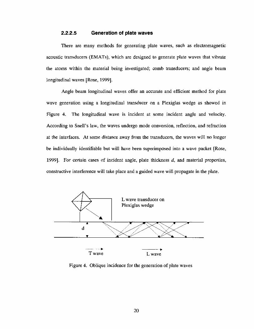
2.2.2.5 Generation of plate waves

There are many methods for generating plate waves, such as electromagnetic

acoustic transducers (EMATs), which are designed to generate plate waves that vibrate

the atoms within the material being investigated; comb transducers; and angle beam

longitudinal waves [Rose, 19991.

Angle beam longitudinal waves offer an accurate and efficient method for plate

wave generation using a longitudinal transducer on a Plexiglas wedge as showed in

Figure 4. The longitudinal wave is incident at some incident angle and velocity.

According to Snell's law, the waves undergo mode conversion, reflection, and refraction

at the interfaces. At some distance away from the transducers, the waves will no longer

be individually identifiable but will have been superimposed into a wave packet [Rose,

19991. For certain cases of incident angle, plate thickness d, and material properties,

constructive interference will take place and a guided wave will propagate in the plate.

. . . . . . . . .. ... . . . .. . b

T wave A

L wave

Figure 4. Oblique incidence for the generation of plate waves

These conditions for constructive interference are actually met for many

combinations of thickness, angle, and material properties. For generation using a

longitudinal wave transducer on a Plexiglas wedge, the phase velocity c p has a simple

relation to the angle of incidence via Snell's law:

sin(oi ) sin(90° ) -- - C~lai~l'Zs

(2.5) P

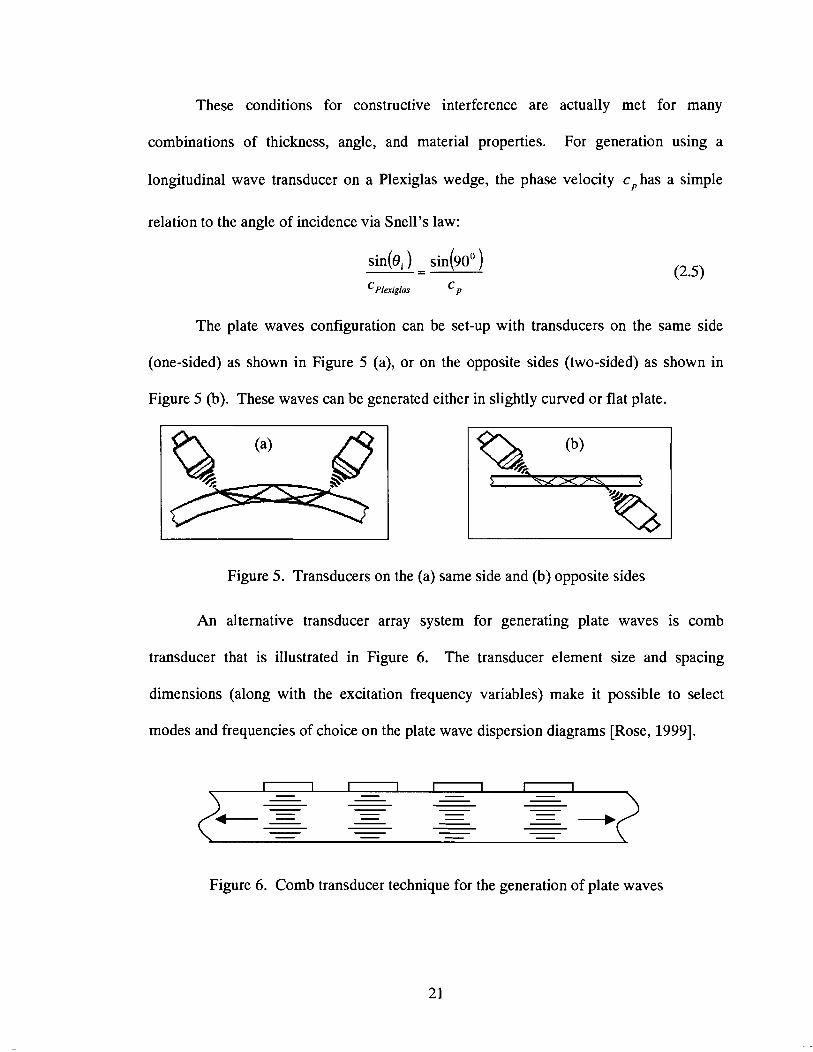
The plate waves configuration can be set-up with transducers on the same side

(one-sided) as shown in Figure 5 (a), or on the opposite sides (two-sided) as shown in

Figure 5 (b). These waves can be generated either in slightly curved or flat plate.

Figure 5. Transducers on the (a) same side and (b) opposite sides

An alternative transducer array system for generating plate waves is comb

transducer that is illustrated in Figure 6. The transducer element size and spacing

dimensions (along with the excitation frequency variables) make it possible to select

modes and frequencies of choice on the plate wave dispersion diagrams [Rose, 19991.

Figure 6. Comb transducer technique for the generation of plate waves

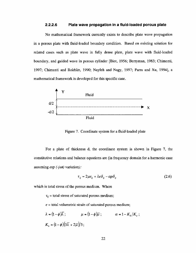
2.2.2.6 Plate wave propagation in a fluid-loaded porous plate

No mathematical framework currently exists to describe plate wave propagation

in a porous plate with fluid-loaded boundary condition. Based on existing solution for

related cases such as plate wave in fully dense plate, plate wave with fluid-loaded

boundary, and guided wave in porous cylinder [Biot, 1956; Berryman, 1983; Chimenti,

1997; Chimenti and Rokhlin, 1990; Nayfeh and Nagy, 1997; Parra and Xu, 19941, a

mathematical framework is developed for this specific case.

f Fluid

-dl2 1 Fluid

Figure 7. Coordinate system for a fluid-loaded plate

For a plate of thickness d, the coordinate system is shown in Figure 7, the

constitutive relations and balance equations are (in frequency domain for a harmonic case

assuming exp (-jwt) variation):

zV = 2peV + LeSij - apSij (2.6)

which is total stress of the porous medium. Where

zq = total stress of saturated porous medium;

e = total volumetric strain of saturated porous medium;

L = (I-@; p = ( 1 - 4 ) ~ ; a = 1 - K,/K, ;

K, = (I - 4)(3n + 2 ~ ) / 3 ;

p = fluid pressure; ) = porosity;

1 and ji are the Lam6 coefficients of the porous skeleton or matrix;

K, and & are the bulk grain modulus and the bulk frame modulus, respectively.

The equations of stress in the pore fluid are:

'T!' = -&dg = ( $ 1 ~ lave u + @v. (U - u)bi ,

where

%* = stress in pore fluid;

u = displacement in the solid frame;

U = displacement in the pores fluid;

P = C - @)ps + ) / K , ;

Kf = pore fluid modulus.

Momentum balance equations for total stress are:

where

p, and pf are the densities of porous matrix and pore fluid, respectively.

The generalized Darcy's law (the average displacement of the fluid relative to the frame)

is:

w = )(u - u ) = e ( a 2 p p , u - vp)

where

e = - K(.)/ j a ;

~ ( a ) is the frequency-dependent generalized Darcy coefficient, and is given by

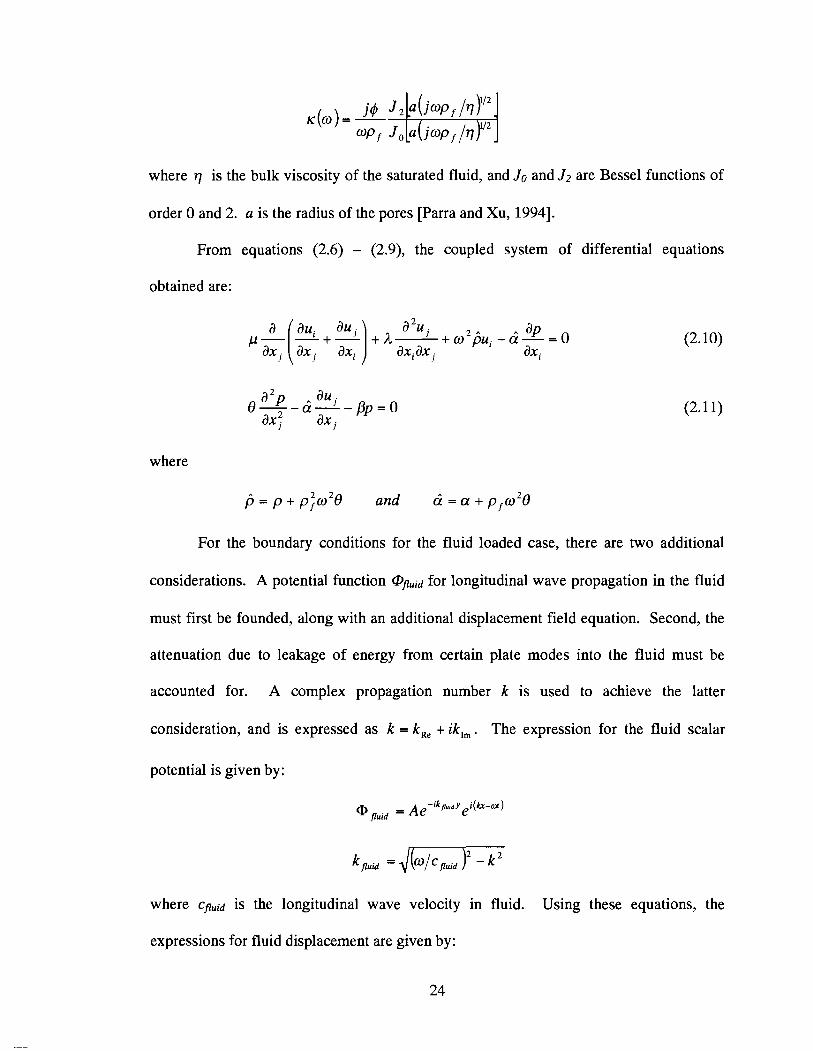
where q is the bulk viscosity of the saturated fluid, and Jo and J2 are Bessel functions of

order 0 and 2. a is the radius of the pores [Parra and Xu, 19941.

From equations (2.6) - (2.9), the coupled system of differential equations

obtained are:

where

1j = p + p ; w 2 0 and oi = a + p f w 2 0

For the boundary conditions for the fluid loaded case, there are two additional

considerations. A potential function @fluid for longitudinal wave propagation in the fluid

must first be founded, along with an additional displacement field equation. Second, the

attenuation due to leakage of energy from certain plate modes into the fluid must be

accounted for. A complex propagation number k is used to achieve the latter

consideration, and is expressed as k = k,, + ik,, . The expression for the fluid scalar

potential is given by:

A e - i k p u 8 d ~ (h -a ) @ fluid = e

where 'fluid is the longitudinal wave velocity in fluid. Using these equations, the

expressions for fluid displacement are given by:

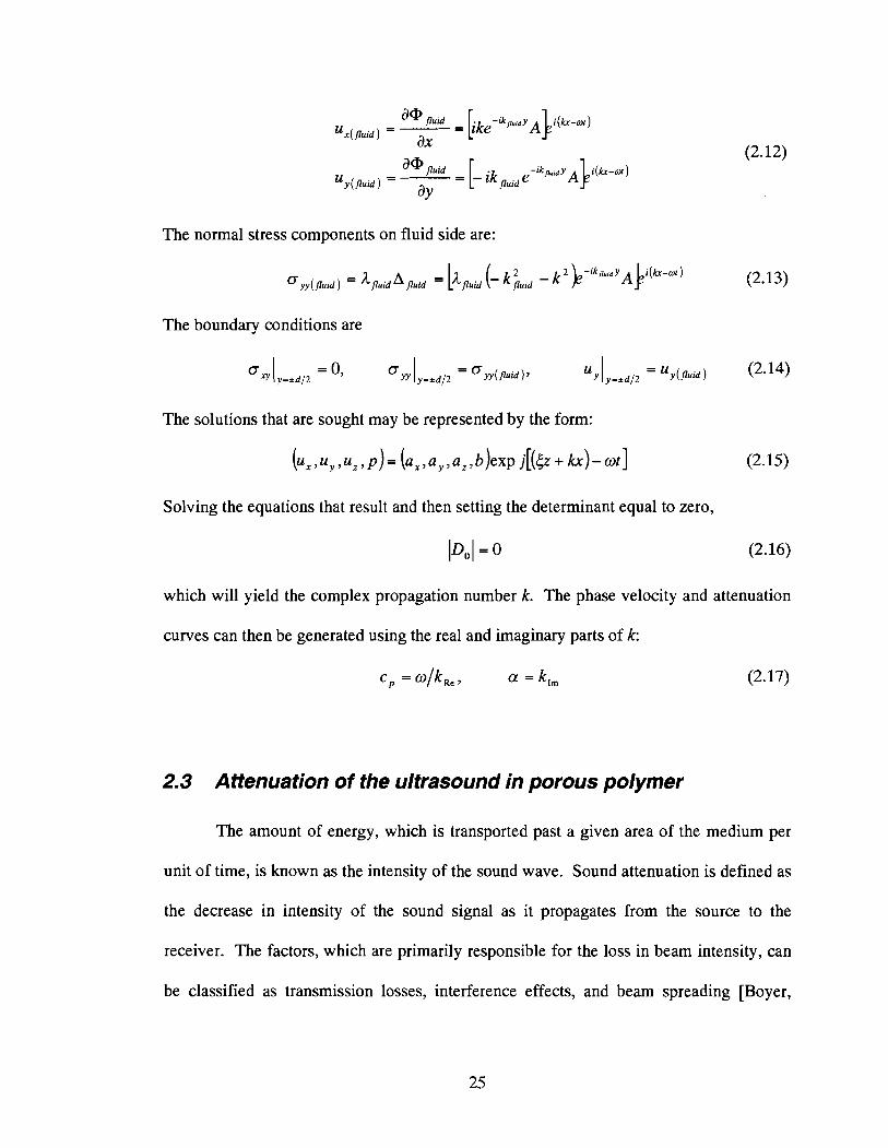
The normal stress components on fluid side are:

k2 ) e - ~ ) 7 u , d y ~ k i ( k X - W ) 'TW(fluid) = 'fluidAfluid = ['fluid (- k;uid - (2.13)

The boundary conditions are

= 0, - 'TXY Iy-*d/2 ly-*d/2 = CT,(fluid), uYly-*d/2 - U ~ ( f l u y ) (2.14)

The solutions that are sought may be represented by the form:

( ~ x , ~ y , ~ z , ~ ) = ( a , , a y , a z , b ) e x p j [ ( ~ + ~ ) - ~ t 1

Solving the equations that result and then setting the determinant equal to zero,

1 ~ 0 1 = 0 (2.16)

which will yield the complex propagation number k. The phase velocity and attenuation

curves can then be generated using the real and imaginary parts of k:

C, = elk,, , a = k,,

2.3 Attenuation of the ultrasound in porous polymer

The amount of energy, which is transported past a given area of the medium per

unit of time, is known as the intensity of the sound wave. Sound attenuation is defined as

the decrease in intensity of the sound signal as it propagates from the source to the

receiver. The factors, which are primarily responsible for the loss in beam intensity, can

be classified as transmission losses, interference effects, and beam spreading [Boyer,

19761. Mostly, attenuation of the ultrasound in porous polymer include scattering by

inhomogeneities, and damping by conversion of the oscillatory motion to heat.

Polymers in general display significant levels of viscoelastic behavior, therefore,

have material damping characteristics that result in measurable attenuation even in the

absence of significant crystallinity. When a sudden stress is applied, the response of

polymer is an instantaneous elastic deformation followed by a delayed deformation. The

delayed deformation is due to various molecular and structural relaxation processes,

which cause the conversion of the sound wave to heat. For a given polymer, damping is

found to depend on the temperature and frequency of the measurements [Corsaro and

Sperling, 19901. Attenuation caused by damping is often observed to increase linearly

with frequency in polymeric solids. This linear increase is observed for both longitudinal

wave and shear wave. It is also found that, at any given frequency, shear wave

attenuation is much higher than longitudinal wave attenuation in viscoelastic materials

[Corsaro and Sperling, 19901.

For porous materials, the scattering by inhomogeneities in a host medium can also

cause attenuation of the ultrasound. The scatterers (pores) can attenuate the ultrasound

wave by any one of the following mechanisms: intrinsic dissipation of ultrasound within

the scatterer itself; mode conversion at the boundary of the scatterer; and scattering of

sound to a back propagating wave [Corsaro and Sperling, 19901. The complete treatment

of the scattering of ultrasound in a porous polymer involves both the calculation of the

scattering cross-section of a single pore in the host medium, and the multiple scattering

effects due to surrounding pores. It is important to note that, in general, scattering of

ultrasound from pores in the polymer does not become significant until the dimensions of

the pores are comparable to the wavelength of ultrasound in the polymer. The frequency

dependency of the attenuation coefficient for scattering depends strongly on the

wavelength relative to the average pore diameter [Schmerr, 19981. Therefore, the

frequency dependence of the attenuation can provide information about the size of the

pores.

Mode conversion at boundaries also causes attenuation of ultrasound. With

appropriate boundary conditions, the longitudinal wave can be converted to shear wave in

the plate or to the viscous flow in the fluid. Conversion to viscous flow is most readily

achieved at the boundaries in porous materials. The viscous flow is then converted to

heat by molecular collisions. The end result is attenuation of the ultrasound wave as it

propagates through the porous materials. The condition is easier to achieve in air than

water [Corsaro and Sperling, 19901. Conversion to shear deformation is particularly

pronounced in materials such as viscoelastic polymers. The shear deformation energy is

converted to heat by molecular relaxation, and the ultrasound wave is attenuated.

Attenuation often serves as a measurement tool that leads to the formation of

theories to explain physical or chemical phenomenon, which decrease the ultrasonic

intensity. Therefore attenuation has the potential to play an important role in

characterization of porous polymer membrane using ultrasound.

2.4 Ultrasonic testing technique

The term ultrasonic testing is used for various testing techniques. The pulse-echo

technique is such that the ultrasound is generated in the part by means of a piezo-electric

transducer, and the reflected signals are recorded by the same transducer. One element in

the probe is configured for both functions (standard probes). The through-transmission

technique is normally applied for a larger wall thickness or material with high sound

absorption. In such case two probes (sender and receiver) are positioned on opposite sides

of the part. Thus the ultrasonic wave only passes one way, and does not require that the

wave pass through the part twice as for the pulse-echo technique.

The difference between the contact technique and the immersion technique is also

a basic consideration for the ultrasonic technique. When using the contact technique the

probe is attached directly to the part. For the acoustic probe-to-specimen contact a

coupling medium must be applied between the probe and the part. This couplant is

typically a viscous gel that can contaminate the material. For ultrasonic testing using the

immersion technique, the transducer is placed in water, which acts as coupling agent

between the part and the transducer. The advantage of the immersion techniques is that

the transducer position may be defined at an optional distance and angle above the part.

Thus considerably higher sensitivity can be achieved in most cases.

3. LITERATURE REVIEW

3.1 Membrane characterization

Membrane formation and characterization have been extensively studied.

Ramaswamy[2002] reviewed the existing techniques employed for the characterization of

membranes. In particular scanning electron microscopy (SEM), bubble point method,

gas permeation (wet and dry-flow method), mercury intrusion method, solution rejection

measurements, and atomic force microscope (AMF) are used to characterize membranes.

Chapter 2 in this work gives more details on each of these methods. Kim et a1 [I9941

compared various techniques, which include thermoporometry, biliquid permporometry,

and molecular weight cut-off determination (MWCO). Khulbe and Matsuura [2000]

reviewed some of the latest techniques, which include Raman spectroscopy (RS),

electron spin resonance (ESR) and atomic force microscopy (AFM). It is clear that there

are many techniques for the characterization of membrane. However, all the techniques

described so far are either destructive, or can only be applied off-line [Ramaswamy

20021. Thus a need for in-site and on-line testing is a continuing need in the field of

membrane science.

3.2 Ultrasonic characterization

The use of ultrasonics for nondestructive characterization of materials has been

widely reported in the literature. Krautkramer and Krautkramer [I9901 presented the

various test problems involving ultrasonic technique. Schmerr [I9981 gave the

fundamentals of ultrasonic nondestructive evaluation in his book. Bray and Stanley

[I9891 showed the developments in ultrasonic techniques in nondestructive evaluation,

and gave large number of problems and the laboratory experiments as examples.

According to these texts, most of the common applications of the ultrasonic testing

involve metallic components (such as casting, welded joints, railway materials, and

nuclear power plant) and non-metallic components, which include detection of the cracks

in glass, bubbles in tires, defects in concrete, bonding in wood, and so on.

Abundant literature exists on the efforts to utilize ultrasonic waves to characterize

the properties of polymers. Hartmann [I9801 reviewed the use of ultrasonic

measurements for polymer solids, and compared the velocities and moduli of different

solid polymers measured by an immersion apparatus. It is well known that polymers are

dispersive materials and that the amount of attenuation is significant. Corsaro and

Sperling [I9901 focused their work on viscoelastic characteristics of solid polymers,

especially the relation between the sound attenuation with the polymer material and

structure. Jones [2001] discussed the damping behavior of polymer materials in his book.

Because of the dispersive characteristics of polymeric materials, the transmitted signals

are deformed and the ultrasonic velocity is frequency dependent. This made

measurements on polymers quite difficult prior to the advent of low cost computers and

digital acquisition. Zellouf et al. [I9961 discussed the application of the Kramers-Kronig

relations to ultrasonic spectroscopy in polymers, and compared attenuation and velocity

spectra by ultrasonic spectroscopy measurement.

3.3 Application of ultrasonic testing to porous materials

Compared to other traditional methods of the porous membrane characterization,

ultrasonic techniques have the advantage of being non-invasive and they are suitable for

on-line testing. This makes ultrasonic techniques potentially one of the most attractive

techniques for porous polymer membrane characterization. Panakkal [I9961 presented an

analysis of experimental data of various types of porous materials and demonstrated the

relationship between ultrasonic velocity and the physical properties of interest. This

paper demonstrated that the measurement of an ultrasonic velocity is useful as a predictor

of diverse material properties of porous materials. Alderson et al. [I9971 described the

experimental study of ultrasonic attenuation in microporous polyethylene. Experiments

were carried out on auxetic (negative Poisson's ratio) microporous ultra-high-molecular

weight polyethylene foams (UHMWPE), and compared to microporous positive

Poisson's ratio UHMWPE and non-porous UHMWPE. The author concluded that the

attenuation in auxetic UHMWPE is higher than non-auxetic UHMWPE; the microporous

polymer, whether auxetic or not, showed strong enhancements in attenuation compared to

the non-porous UHMWPE.

Johnson et a1 [I9871 studied the response of a simple fluid entrained in a rigid

porous medium and subjected to a harmonic pressure drop across the sample. In their

work, they showed the relevant response functions, the dynamic permeability and

tortuosity in fluid-saturated porous materials, were analytic functions of frequency. A

parameter A was defined, which dynamically connected with pore size. To measure the

dynamic permeability/tortuosity of porous material, Helium was used to fill the pores.

Based on this research, Johnson et a1 [1994; 19941 reported the measurements of phase

velocity and attenuation of first and second sound as function of frequency and

temperature in different cases. These measurements were in excellent agreement with the

theoretical predictions.

More directly relevant research has also been done with membrane materials.

Kools et a1 [I9981 made efforts to extending the applicability of ultrasonics for real time

measurement of thickness changes during evaporative casting of polymeric membranes.

These experiments were preformed using pulse-echo system and a 10MHz transducer.

Longitudinal waves were reflected at the top and bottom surface of the membrane. The

arrival time of the various reflected signals was used to determine the thickness of the

membrane. Peterson et a1 [I9981 developed ultrasonic time-domain reflectometry (TDR)

for quantifying membrane compressive strain. The major limitation of previous

compaction studies was the inability to obtain the measurements at the same time as

permeating flux and membrane thickness changes were monitored in real time. As the

result, compressive strain had to be obtained indirectly. In this work, the authors

employed a pulse-echo ultrasound system, and a 25MHz transducer was used to measure

the arrival time of reflection signal from membrane. The strain measurement was based

on the change in arrival time, which translated into changes in membrane thickness

during compaction. These studies and ongoing work point to the importance of

ultrasonic methods in the membrane characterization.

Another important area for ultrasonics is in membrane fouling [Lloyd, 19851.

Fouling is a major problem that limits membrane application. Maria1 et a1 [1999; 20001

described an approach to the real-time, noninvasive, in situ measurement of membrane

fouling layer growth and cleaning using ultrasonic time-domain reflectometry. The

fouling layer was present on the membrane, and altered the reflected ultrasonic signal

generated by a transducer. The same approach was utilized as the measurement of

thickness changes. Li and Sanderson [2002] showed that the ultrasonic technique could

be used for in situ measurement of particles deposition and removal, and also could be

used to monitor membrane cleaning.

Defect detection is the third area of membrane science with important implication

for ultrasonic testing. Ramaswamy [2002] focused his work on adapting the ultrasonic

time-domain reflectometry (UTDR) technique for study and characterization of

membrane structure. He showed that the velocity and amplitude of reflected ultrasonic

waves are greatly altered by the presence of defects in the membrane structure, and

evaluated the ability of the UTDR technique to identify the defects with a wide range of

size-scales including pinholes and macrovoids. A 90MHz ultrasonic transducer was used

in his work to successfully obtain unique acoustic signatures from microporous

polymeric membranes of three different sub-micron pore sizes.

With the potential broad implications of this technology, it is particularly

important that a fundamental understanding be developed. The theoretical foundations

do exist and can be applied to this problem.

3.4 Biot 's theory

Biot [I9561 developed a phenomenological model of wave propagation in fluid-

saturated porous media to model the propagation of ultrasonic waves through porous

materials. These equations were derived based on the assumptions that the wavelength is

much larger than the pore scale, and the solid matrix is isotropic. These are reasonable

assumptions when normal ultrasonic frequencies are used with microporous membranes.

Plona [I9801 first used an ultrasonic immersion technique to generate the two bulk

longitudinal modes in a fluid-saturated porous medium. Experiments were carried out

using water and sintered glass spheres. A second bulk compressional wave, which

propagates at a speed that is approximately 25% of the speed of the normal bulk wave,

was observed. Plona's study confirmed the existence of the three waves predicted by

Biot. Berryman [I9801 demonstrated quantitative agreement between Biot's theory and

Plona's measurement, and thus, concluded that Biot's theory provided an accurate

description of elastic wave propagation in fluid-saturated porous media.

Based on the classical work of Biot, a number of efforts to extend the application

of Biot's equations have occurred. Biot's theory has a significant restriction to a fully

saturated solid. Therefore, the applications of Biot's equations were limited in many

problems of practical interest in geophysics and materials science. Berryman and

Thigpen [I9851 developed a comprehensive theory of partially saturated solids at low

frequencies, thus, reducing the limitations of Biot's theory of full saturation. Brown and

Korringa [I9751 derived theoretical formulas relating the elastic moduli of an anisotropic

dry rock to the same rock containing fluid [Mavko et al, 19981, which extend Biot's

theory to anisotropic materials.

Berryman [I9831 studied ultrasonic dispersion of extensional waves in fluid-

saturated porous cylinders by analyzing generalized Pochhammer equations derived

using Biot's theory. He considered the cases with open-pore surface and closed-pore

surface boundary conditions. He found the fast extensional wave didn't differ much, and

a slow wave propagated in the case with a closed-pore surface but not in the case with

open-pore surface.

Wu et a1 [I9901 solved the wave equation, and developed a theoretical analysis to

determine the reflection and transmission coefficients of elastic waves from a fluid

saturated porous solid boundary. Two cases of modes conversion were studied: (1) wave

incident from the fluid, and generated three transmitted waves in the fluid saturated

porous solid; (2) wave incident from the fluid saturated porous media to the interface,

and the generated the three reflected waves in the same media. This work also showed

that the open-pore and sealed-pore boundary caused a significant difference in the

reflection and transmission characteristics of the elastic waves.

Biot's theory has been primarily applied to problems involving geological

applications including viscoelastic materials and partially saturated materials

[Ramaswamy, 20021. Stoll [1977; 19801 has studied the propagation of acoustic waves

in ocean sediments. Based on Biot's theory, the propagation of acoustic waves in

sediments was modeled to predict the velocity and attenuation of the waves. Mavko et a1

[I9981 brought together much of the theory to form the foundation of rock physics with

particular emphasis on wave propagation, effective material, and elasticity and

poroelasticity. With the exception of Berrymen's work on porous cylinder [Berrymen,

19831, no previous work on porous materials has considered guided waves in porous

media.

3.5 Plate wave (Lamb wave)

Plate and other guided waves have been used in many ultrasonic applications.

Guided waves, waves that travel along a surface, a rod, a tube, or a plate-like structure,

could be much more efficient than the traditional technique of point-by-point

examination [Rose, 19991. Guided wave techniques can be used to find tiny defects over

large distance, under adverse condition, in structures with coatings, and in harsh

environments. Guided wave concepts have been extended to help examine the

composites on the aircraft, the tubing in power plants, the pipelines in chemical

processing facilities, and the safety aspects of large petroleum and gas pipelines

[Chimenti, 1997; Rose 19991. All the research or tests applied on porous membrane

using ultrasonic waves described so far are normally incident.

A number of researchers have made efforts to develop and extend the

applicability of guided plate waves. Redwood [I9601 emphasized work on the theoretical

analysis of guided waves, and considered both fluid and solid waveguides. Achenbach

[I9831 gives a detailed mathematical background for guided waves propagating in plates,

layers, and rods. Krautkramer and Krautkramer [I9831 describes the physical principles

of the plate wave, and discusses practical testing techniques using plate waves for steep

plate, sheet, strip, rod and wires. Rose [I9991 explained the basic physical principles of

wave propagation, and then related them to the more recent guided wave techniques used

for inspection and evaluation. Seale et a1 [I9941 showed that Lamb wave's velocity

could be used to evaluate fatigued composites, and thermally damaged composites.

Chimenti [I9971 gives a more current review of ultrasonic characterization of materials

using guided plate waves and describes their usage to evaluate the mechanical properties

of both isotropic and anisotropic plates.

Methods of presenting the guided wave behavior in plates represent an additional

challenge from a practical perspective. Dayal and Afful [I9931 presented a technique for

plate wave velocity and attenuation measurement. This technique is based on the

conversion of the time domain signal into frequency domain. Since the calculation was

made in frequency domain, the dispersive nature of the plate waves can be detected and

measured. This technique was applied to an aluminum plate of thickness 1.57mm, and a

metal-matrix (SiCtTi) sample. The experimental result showed very good correlation

with theoretically determined curves in the dispersive regions.

Alleyne and Cawley [I9911 demonstrated the application of the 2D Fourier

transform for analyzing multimode time signals. Chapter 2 gives details about this

method. The advantage of this method is that the different modes are more easily

distinguished in the wavenumber-angular frequency domain. The limitation of this

method is the requirement of a signal discretized in space and time [Niethammer, 19991.

In contrast to the 2D Fourier transform, time-frequency representation method

only needs a single 1D signal. Nietharnmer and Jacobs [2000] reported a study that

applied the reassigned spectrogram to develop the dispersion curve for Lamb (plate)

wave propagation in an aluminum plate. This study showed that this technique was

extremely effective in localizing multiple, closely spaced modes in both time and

frequency. Further more, Niethammer et a1 [2001] compared the effectiveness of four

candidate time frequency representations to analyze broadband multimode ultrasonic

waves. The four methods were the reassigned spectrogram, the reassigned scalogram, the

smoothed Wiper-Ville distribution, and the Hilbert spectrum. The result showed that

each method had certain advantages and disadvantages, but the reassigned spectrogram

was the best method to characterize Lamb waves.

These recent methods of describing the complex signals produced during plate

wave inspection are quite important for modern testing. Dispersive signals are only

tractable with the appropriate analysis. However, as opposed to simpler signals, plate

waves contain significant information about the materials and the condition of the

sample.

3.6 Water loading influence on guided waves

A Lamb wave is generated for traction free boundary conditions. However, for

practical ultrasonics water immersion is required to generate the wave. Thus, it is of

interest to find the behavior of the plate immersed in water. The propagation of guided

waves is impacted by the effect of water loading because reflection at the plate water

interface is not complete. The fluid loaded plate wave, which is called leaky Lamb wave

(LLW), refers to the tendency for energy to leak from the plate. The phenomenon is a

resonant excitation of plate waves that leak waves into the immersion fluid [Rose, 19991.

The leaky Lamb wave phenomenon has been an important topic for at least two decades,

and led numerous studies of ultrasonic wave propagation with fluid loading.

Billy et a1 [I9841 observed backscattered leaky Lamb waves from a plate

immersed in liquid. These backward propagation Lamb waves leak back at both sides of

the plate. Dayal and Kinra [I9891 considered the propagation of leaky Lamb wave in a

composite plate. An exact solution and numerical result were obtained and were shown

to be in good agreement with experments. Xu et a1 [I9931 applied the leaky Lamb wave

technique to the quantitative characterization of coatings, and showed the potential ability

of leaky Lamb wave for real time inspection. Nayfeh and Nagy [I9971 extended the

analytical model to assess the effect of viscous fluid loading on Lamb wave properties

when it is propagating in fluid-loaded solid.

In a review paper, Chimenti [I9971 introduced some phenomenological aspects of

plate waves and several approaches to the mathematical modeling. Chimenti gives a

detailed discussion of a partial wave analysis in an anisotropic fluid-loaded plate. Several

analytical and finite element or finite difference approaches have been used for plate

wave modeling of water-loaded cases. Depending on the applications, advantages and

weaknesses of these models exist.

Rose [I9991 also gives a more physical explanation of the effect from the water

loading in his book. Examples of leaky guided waves from water-loaded hollow cylinder

are shown as well as the possibility of using various numerical techniques for this

problem.

3.7 Summary

From brief review of the literature, it is clear that the application of ultrasonics for

the characterization of the porous materials and membranes is an important emerging

area. The ability of Biot7s theory to predict pore sizes from wave propagation parameters

presents an important role for NDT in porous membranes using ultrasonic waves. The

fluid loaded case for fully dense plate wave propagation has also been considered.

Because of the complexity of the problem, no previous discussion of the modeling of

plate wave propagation in porous materials with fluid loading has been found. This is the

case for both experimental and theoretical studies of the topic.

4. SIGNAL PROCESSING

4. I Attenuation measurement using deconvolution and

Pseudo- Wiener filter

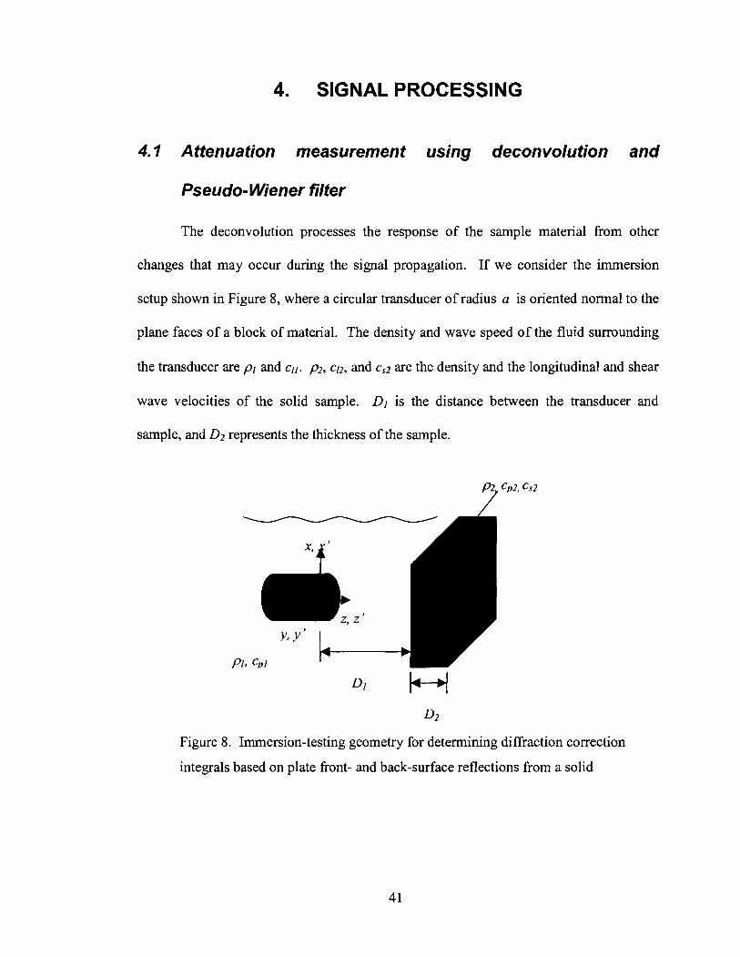
The deconvolution processes the response of the sample material from other

changes that may occur during the signal propagation. If we consider the immersion

setup shown in Figure 8, where a circular transducer of radius a is oriented normal to the

plane faces of a block of material. The density and wave speed of the fluid surrounding

the transducer are pl and ell. p2, ~ 1 2 , and c,2 are the density and the longitudinal and shear

wave velocities of the solid sample. Dl is the distance between the transducer and

sample, and D2 represents the thickness of the sample.

D2

Figure 8. Immersion-testing geometry for determining diffraction correction

integrals based on plate front- and back-surface reflections from a solid

For the front- and back-surface responses, we have the received voltages:

where a, and a, are the attenuation coefficients for the water and the solid, respectively.

P(o) is a frequency-dependent input proportionality factor. p,fe and pEe are spatially

averaged received pressure for front- and back-surface, and vo is the frequency response

of the spatially uniform velocity over the face of the transducer [Schmerr, 19981.

In principle, we can obtain the attenuation of the solid from:

where

where RZP, TI;:', and TgtP denote the reflection coefficient from fluid to solid, the

transmission coefficient from fluid to solid, and the transmission coefficient from solid to

fluid, respectively. All of these three coefficients denote the transmitted longitudinal

wave due to an incident longitudinal wave. Dl is a diffraction correction term, and

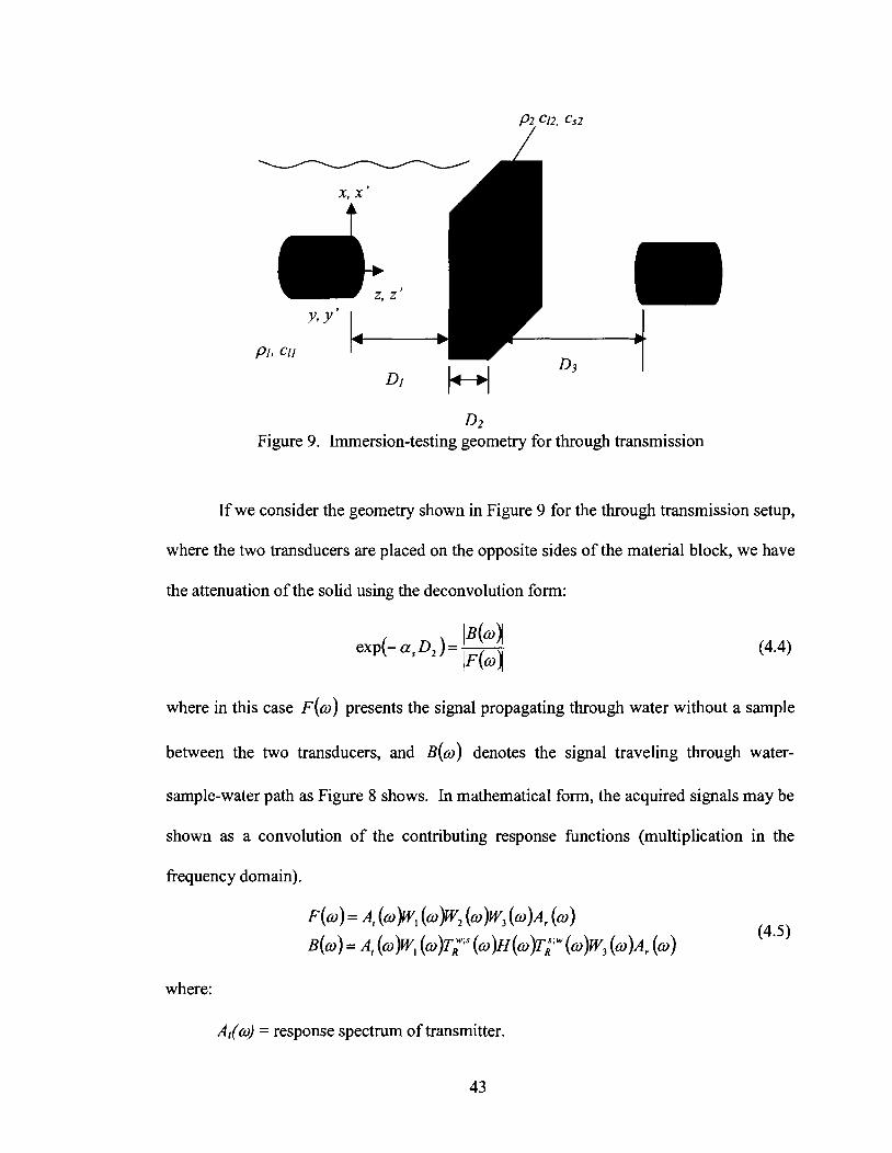
D2 Figure 9. Immersion-testing geometry for through transmission

If we consider the geometry shown in Figure 9 for the through transmission setup,

where the two transducers are placed on the opposite sides of the material block, we have

the attenuation of the solid using the deconvolution form:

where in this case ~ ( w ) presents the signal propagating through water without a sample

between the two transducers, and ~ ( o ) denotes the signal traveling through water-

sample-water path as Figure 8 shows. In mathematical form, the acquired signals may be

shown as a convolution of the contributing response functions (multiplication in the

frequency domain).

where:

A,(&) = response spectrum of transmitter.

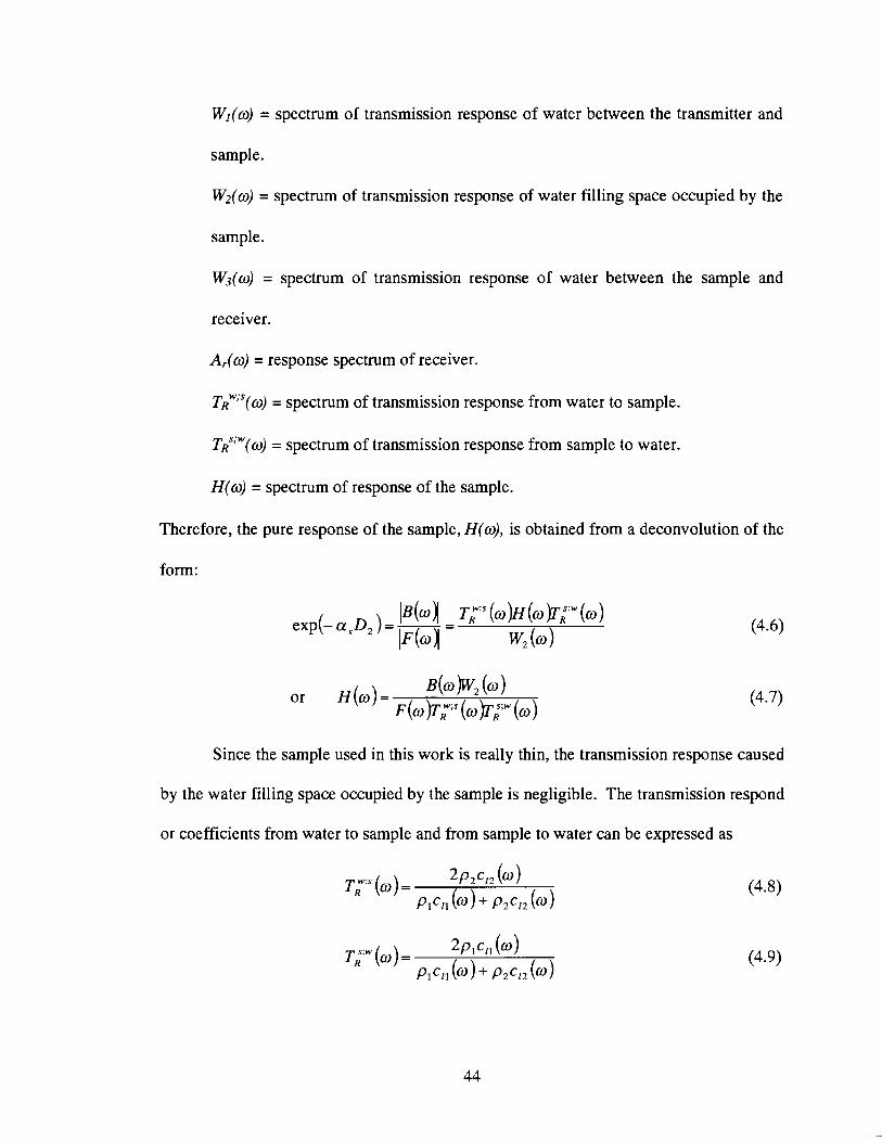
Wl(w) = spectrum of transmission response of water between the transmitter and

sample.

W2(0) = spectrum of transmission response of water filling space occupied by the

sample.

W3(0) = spectrum of transmission response of water between the sample and

receiver.

A,(o) = response spectrum of receiver.

T R ~ ; ~ ( O ) = spectrum of transmission response from water to sample.

T R ~ ' ~ ( O ) = spectrum of transmission response from sample to water.

H(w) = spectrum of response of the sample.

Therefore, the pure response of the sample, H(o), is obtained from a deconvolution of the

form:

or ~ ( m ) = ~ ( 0 )W2 (0 ) F (m )Ti;, (a )Tiiw (m)

Since the sample used in this work is really thin, the transmission response caused

by the water filling space occupied by the sample is negligible. The transmission respond

or coefficients from water to sample and from sample to water can be expressed as

T;, (m) = 2 ~ 2 ~ 1 2 (4 P l c l l (4 + ~ 2 ~ 1 2 (4

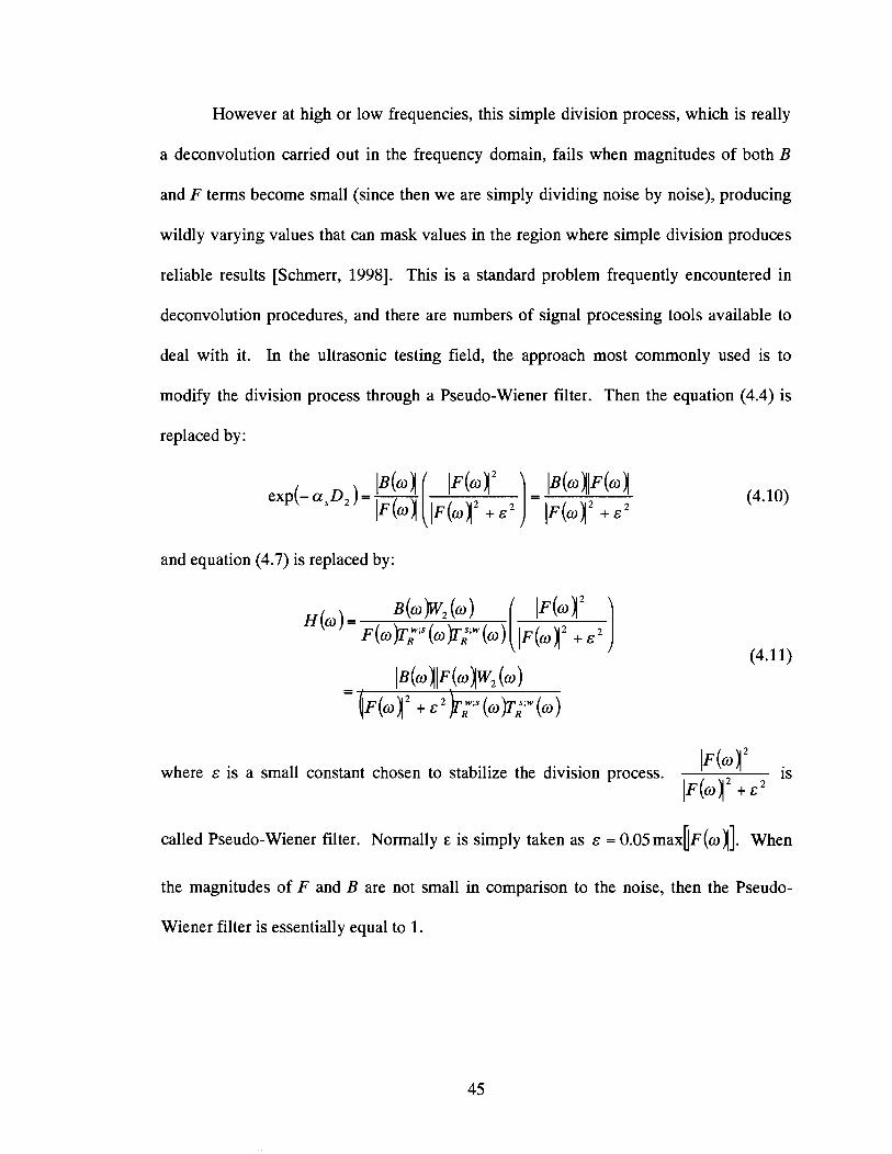
However at high or low frequencies, this simple division process, which is really

a deconvolution carried out in the frequency domain, fails when magnitudes of both B

and F terms become small (since then we are simply dividing noise by noise), producing

wildly varying values that can mask values in the region where simple division produces

reliable results [Schmerr, 19981. This is a standard problem frequently encountered in

deconvolution procedures, and there are numbers of signal processing tools available to

deal with it. In the ultrasonic testing field, the approach most commonly used is to

modify the division process through a Pseudo-Wiener filter. Then the equation (4.4) is

replaced by:

and equation (4.7) is replaced by:

where E is a small constant chosen to stabilize the division process. p(o)12 is

IF(w)(' + c 2

called Pseudo-Wiener filter. Normally E is simply taken as E = 0.05 max[lF (w I]. When

the magnitudes of F and B are not small in comparison to the noise, then the Pseudo-

Wiener filter is essentially equal to 1.

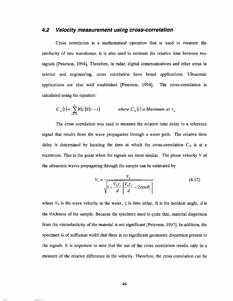
4.2 Velocity measurement using cross-correlation

Cross correlation is a mathematical operation that is used to measure the

similarity of two waveforms. It is also used to estimate the relative time between two

signals [Peterson, 19941. Therefore, in radar, digital communications and other areas in

science and engineering, cross correlation have broad applications. Ultrasonic

applications are also well established [Peterson, 19941. The cross-correlation is

calculated using the equation:

The cross correlation was used to measure the relative time delay to a reference

signal that results from the wave propagation through a water path. The relative time

delay is determined by locating the time at which the cross-correlation C , is at a

maximum. This is the point when the signals are most similar. The phase velocity V of

the ultrasonic waves propagating through the sample can be estimated by

\I I + - - - Vzi [Vzi 2 cos 8, I where Vo is the wave velocity in the water, Ti is time delay, Oi is the incident angle, d is

the thickness of the sample. Because the specimen used is quite thin, material dispersion

from the viscoelasticity of the material is not significant [Peterson, 19971. In addition, the

specimen is of sufficient width that there is no significant geometric dispersion present in

the signals. It is important to note that the use of the cross correlation results only in a

measure of the relative difference in the velocity. Therefore, the cross correlation can be

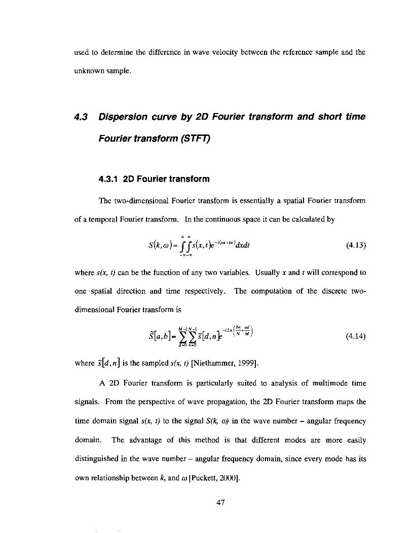
used to determine the difference in wave velocity between the reference sample and the

unknown sample.

4.3 Dispersion curve by 2 0 Fourier transform and short time

Fourier transform (ST-

4.3.1 2D Fourier transform

The two-dimensional Fourier transform is essentially a spatial Fourier transform

of a temporal Fourier transform. In the continuous space it can be calculated by

where s(x, t) can be the function of any two variables. Usually x and t will correspond to

one spatial direction and time respectively. The computation of the discrete two-

dimensional Fourier transform is

M - I N - I [t K") ?[a, b]= 2 S [ d , n ~ p - ~ ~ ~ + - n-

where S[d,n] is the sampled s(x, t) [Niethammer, 19991.

A 2D Fourier transform is particularly suited to analysis of multimode time

signals. From the perspective of wave propagation, the 2D Fourier transform maps the

time domain signal s(x, t) to the signal S(k, w) in the wave number - angular frequency

domain. The advantage of this method is that different modes are more easily

distinguished in the wave number - angular frequency domain, since every mode has its

own relationship between k, and w [Puckett, 20001.

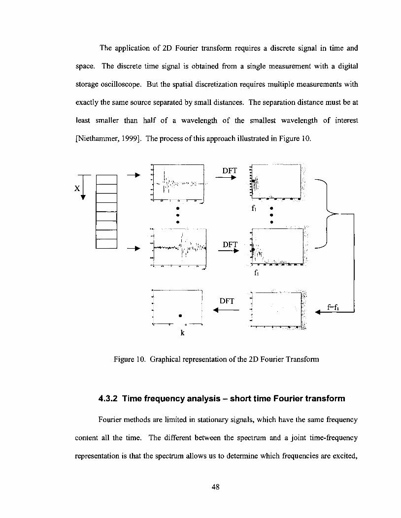
The application of 2D Fourier transform requires a discrete signal in time and

space. The discrete time signal is obtained from a single measurement with a digital

storage oscilloscope. But the spatial discretization requires multiple measurements with

exactly the same source separated by small distances. The separation distance must be at

least smaller than half of a wavelength of the smallest wavelength of interest

[Niethamrner, 19991. The process of this approach illustrated in Figure 10.

4.

I

as. r l . ) I ) I .

-b i', s~, i ; , ' )s:k DFT I / ' , i

~

, , -

0. ; ,* , >. 4 . "*

J fl

DFT +

Figure 10. Graphical representation of the 2D Fourier Transform

4.3.2 Time frequency analysis - short time Fourier transform

Fourier methods are limited in stationary signals, which have the same frequency

content all the time. The different between the spectrum and a joint time-frequency

representation is that the spectrum allows us to determine which frequencies are excited,

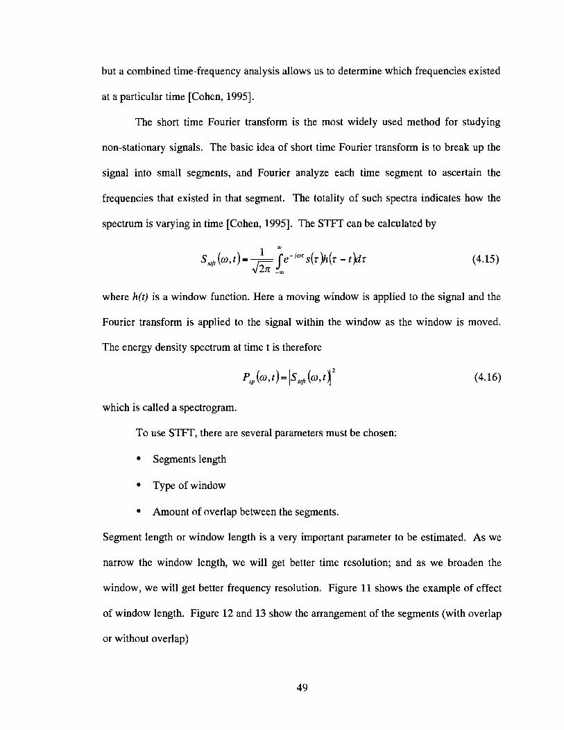
but a combined time-frequency analysis allows us to determine which frequencies existed

at a particular time [Cohen, 19951.

The short time Fourier transform is the most widely used method for studying

non-stationary signals. The basic idea of short time Fourier transform is to break up the

signal into small segments, and Fourier analyze each time segment to ascertain the

frequencies that existed in that segment. The totality of such spectra indicates how the

spectrum is varying in time [Cohen, 19951. The STFT can be calculated by

where h(t) is a window function. Here a moving window is applied to the signal and the

Fourier transform is applied to the signal within the window as the window is moved.

The energy density spectrum at time t is therefore

psp (w 4 = Iss@ (01 j2

which is called a spectrogram.

To use STFT, there are several parameters must be chosen:

Segments length

Type of window

Amount of overlap between the segments.

Segment length or window length is a very important parameter to be estimated. As we

narrow the window length, we will get better time resolution; and as we broaden the

window, we will get better frequency resolution. Figure 11 shows the example of effect

of window length. Figure 12 and 13 show the arrangement of the segments (with overlap

or without overlap)

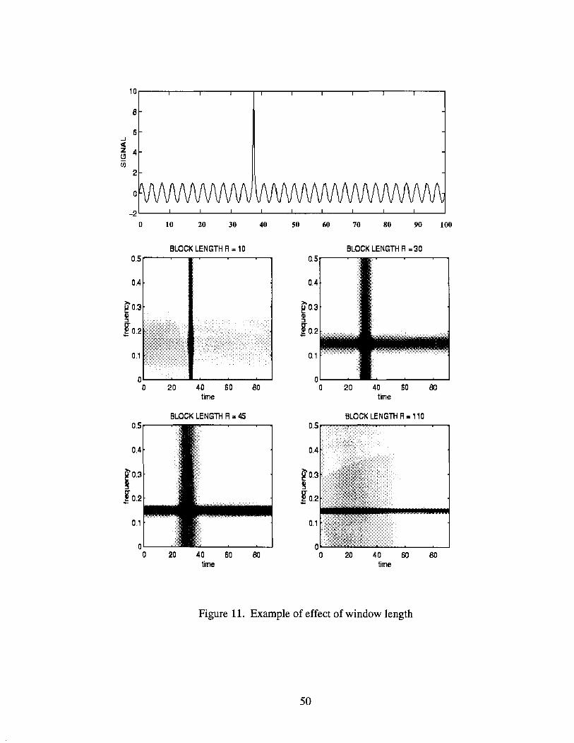
BLOCK LENGTH R = 10 BLOCK LENGTH R =30

0 20 40 60 80 time

BLOCK LENGTH R = 45

0 20 40 60 80 time

0 20 40 60 80 time

BLOCK LENGTH R = 110

0 20 40 60 80 time

Figure 11. Example of effect of window length

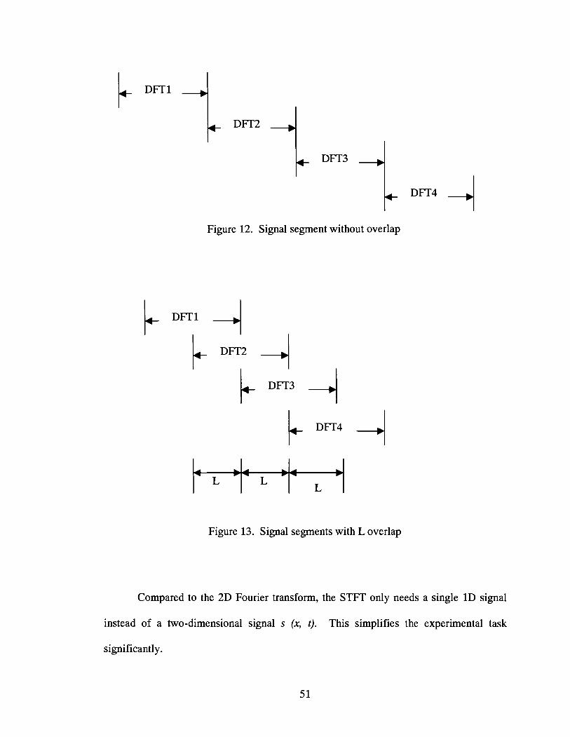
Figure 12. Signal segment without overlap

Figure 13. Signal segments with L overlap

Compared to the 2D Fourier transform, the STFT only needs a single 1D signal

instead of a two-dimensional signal s (x, t). This simplifies the experimental task

significantly.

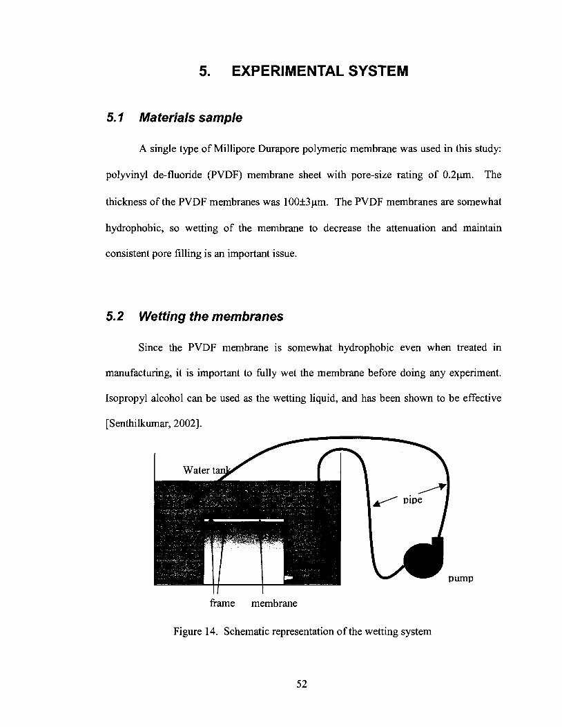
5. EXPERIMENTAL SYSTEM

5. I Materials sample

A single type of Millipore Durapore polymeric membrane was used in this study:

polyvinyl de-fluoride (PVDF) membrane sheet with pore-size rating of 0.2pm. The

thickness of the PVDF membranes was 100f 3pm. The PVDF membranes are somewhat

hydrophobic, so wetting of the membrane to decrease the attenuation and maintain

consistent pore filling is an important issue.

5.2 Wetting the membranes

Since the PVDF membrane is somewhat hydrophobic even when treated in

manufacturing, it is important to hlly wet the membrane before doing any experiment.

Isopropyl alcohol can be used as the wetting liquid, and has been shown to be effective

[Senthilkumar, 20021.

frame membrane

Figure 14. Schematic representation of the wetting system

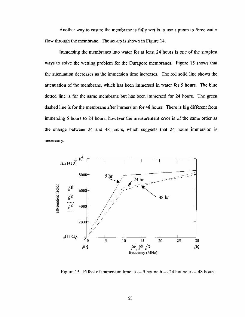
Another way to ensure the membrane is fully wet is to use a pump to force water

flow through the membrane. The set-up is shown in Figure 14.

Immersing the membranes into water for at least 24 hours is one of the simplest

ways to solve the wetting problem for the Durapore membranes. Figure 15 shows that

the attenuation decreases as the immersion time increases. The red solid line shows the

attenuation of the membrane, which has been immersed in water for 5 hours. The blue

dotted line is for the same membrane but has been immersed for 24 hours. The green

dashed line is for the membrane after immersion for 48 hours. There is big different from

immersing 5 hours to 24 hours, however the measurement error is of the same order as

the change between 24 and 48 hours, which suggests that 24 hours immersion is

necessary.

(d (d (d a ,b ,c 30

frequency (MHz)

Figure 15. Effect of immersion time. a --- 5 hours; b --- 24 hours; c --- 48 hours

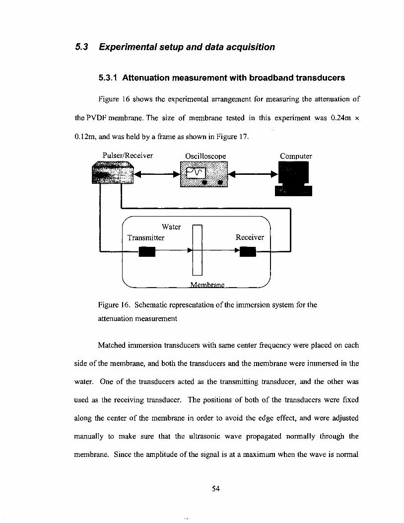
5.3 Experimental setup and data acquisition

5.3.1 Attenuation measurement with broadband transducers

Figure 16 shows the experimental arrangement for measuring the attenuation of

the PVDF membrane. The size of membrane tested in this experiment was 0.24m x

0.12m, and was held by a frame as shown in Figure 17.

Pulser/Receiver Oscilloscope Computer

Figure 16. Schematic representation of the immersion system for the

attenuation measurement

I

Matched immersion transducers with same center frequency were placed on each

side of the membrane, and both the transducers and the membrane were immersed in the

water. One of the transducers acted as the transmitting transducer, and the other was

used as the receiving transducer. The positions of both of the transducers were fixed

along the center of the membrane in order to avoid the edge effect, and were adjusted

manually to make sure that the ultrasonic wave propagated normally through the

membrane. Since the amplitude of the signal is at a maximum when the wave is normal

Water Transmitter

e

-

-

Receiver

b--W

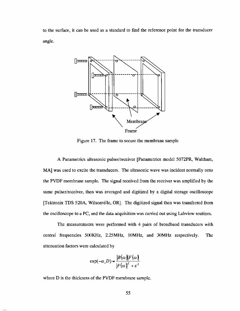
to the surface, it can be used as a standard to find the reference point for the transducer

angle.

Figure 17. The frame to secure the membrane sample

A Panarnetrics ultrasonic pulserlreceiver [Panametrics model 5072PR, Waltham,

MA] was used to excite the transducers. The ultrasonic wave was incident normally onto

the PVDF membrane sample. The signal received from the receiver was amplified by the

same pulserlreceiver, then was averaged and digitized by a digital storage oscilloscope

[Tektronix TDS 520A, Wilsonville, OR]. The digitized signal then was transferred from

the oscilloscope to a PC, and the data acquisition was carried out using Labview routines.

The measurements were performed with 4 pairs of broadband transducers with

central frequencies SOOKHz, 2.25MHz, lOMHz, and 30MHz respectively. The

attenuation factors were calculated by

where D is the thickness of the PVDF membrane sample.

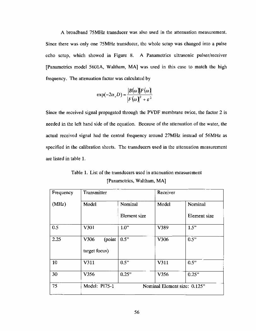
A broadband 75MHz transducer was also used in the attenuation measurement.

Since there was only one 75MHz transducer, the whole setup was changed into a pulse

echo setup, which showed in Figure 8. A Panametrics ultrasonic pulserlreceiver

[Panametrics model 5601A, Waltham, MA] was used in this case to match the high

frequency. The attenuation factor was calculated by

Since the received signal propagated through the PVDF membrane twice, the factor 2 is

needed in the left hand side of the equation. Because of the attenuation of the water, the

actual received signal had the central frequency around 27MHz instead of 56MHz as

specified in the calibration sheets. The transducers used in the attenuation measurement

are listed in table 1.

Table 1. List of the transducers used in attenuation measurement

[Panametrics, Waltham, MA]

Frequency

(MHz)

0.5

2.25

10

30

Transmitter

75

Receiver

Model: PI75-1 Nominal Element size: 0.125"

Model

V30 1

V306 (point

target focus)

V311

V356

Model

V389

V306

V311

V356

Nominal

Element size

1.0"

0.5"

0.5"

0.25"

Nominal

Element size

1.5"

0.5"

0.5"

0.25"

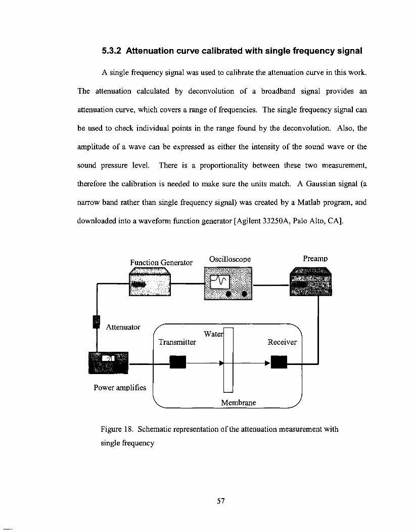
5.3.2 Attenuation curve calibrated with single frequency signal

A single frequency signal was used to calibrate the attenuation curve in this work.

The attenuation calculated by deconvolution of a broadband signal provides an

attenuation curve, which covers a range of frequencies. The single frequency signal can

be used to check individual points in the range found by the deconvolution. Also, the

amplitude of a wave can be expressed as either the intensity of the sound wave or the

sound pressure level. There is a proportionality between these two measurement,

therefore the calibration is needed to make sure the units match. A Gaussian signal (a

narrow band rather than single frequency signal) was created by a Matlab program, and

downloaded into a waveform function generator [Agilent 33250A, Palo Alto, CAI.

Attenuator

Power amplifies 1 U Membrane

Figure 18. Schematic representation of the attenuation measurement with

single frequency

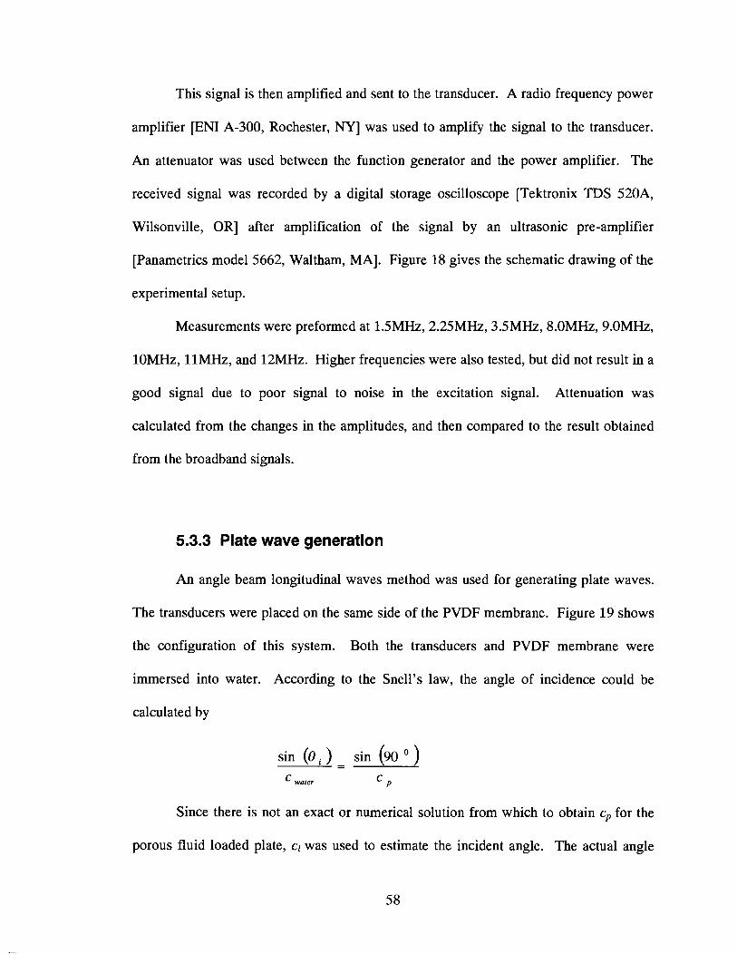
This signal is then amplified and sent to the transducer. A radio frequency power

amplifier [EN1 A-300, Rochester, NY] was used to amplify the signal to the transducer.

An attenuator was used between the function generator and the power amplifier. The

received signal was recorded by a digital storage oscilloscope [Tektronix TDS 520A,

Wilsonville, OR] after amplification of the signal by an ultrasonic pre-amplifier

[Panametrics model 5662, Waltham, MA]. Figure 18 gives the schematic drawing of the

experimental setup.

Measurements were preformed at lSMHz, 2.25MHz, 3.5MHz, 8.0MHz, 9.0MHz,

lOMHz, l lMHz, and 12MHz. Higher frequencies were also tested, but did not result in a

good signal due to poor signal to noise in the excitation signal. Attenuation was

calculated from the changes in the amplitudes, and then compared to the result obtained

from the broadband signals.

5.3.3 Plate wave generation

An angle beam longitudinal waves method was used for generating plate waves.

The transducers were placed on the same side of the PVDF membrane. Figure 19 shows

the configuration of this system. Both the transducers and PVDF membrane were

immersed into water. According to the Snell's law, the angle of incidence could be

calculated by

sin (e ) sin (90 ) - -

Since there is not an exact or numerical solution from which to obtain c, for the

porous fluid loaded plate, cl was used to estimate the incident angle. The actual angle

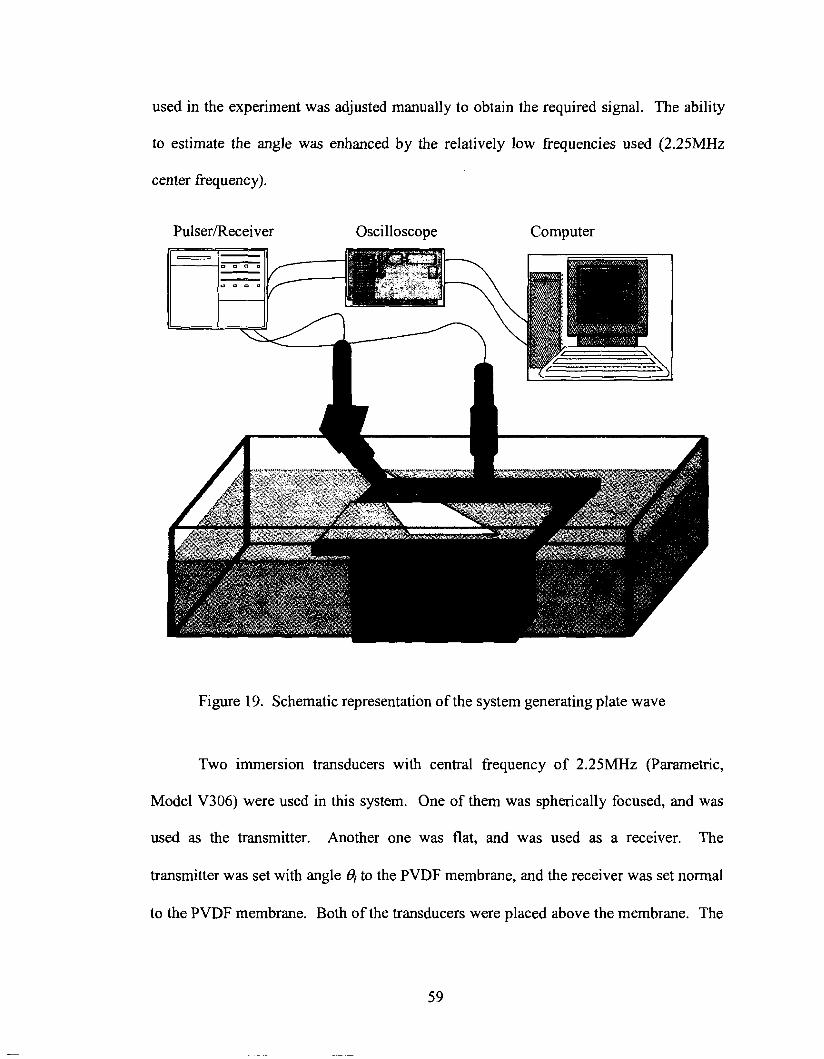
used in the experiment was adjusted manually to obtain the required signal. The ability

to estimate the angle was enhanced by the relatively low frequencies used (2.25MHz

center frequency).

PulserIReceiver Oscilloscope Computer

Figure 19. Schematic representation of the system generating plate wave

Two immersion transducers with central frequency of 2.25MHz (Parametric,

Model V306) were used in this system. One of them was spherically focused, and was

used as the transmitter. Another one was flat, and was used as a receiver. The

transmitter was set with angle 4 to the PVDF membrane, and the receiver was set normal

to the PVDF membrane. Both of the transducers were placed above the membrane. The

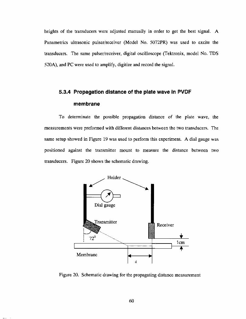
heights of the transducers were adjusted manually in order to get the best signal. A

Panametrics ultrasonic pulser/receiver (Model No. 5072PR) was used to excite the

transducers. The same pulser/receiver, digital oscilloscope (Tektronix, model No. TDS

520A), and PC were used to amplify, digitize and record the signal.

5.3.4 Propagation distance of the plate wave in PVDF

membrane

To determinate the possible propagation distance of the plate wave, the

measurements were preformed with different distances between the two transducers. The

same setup showed in Figure 19 was used to perform this experiment. A dial gauge was

positioned against the transmitter mount to measure the distance between two

transducers. Figure 20 shows the schematic drawing.

, Holder

Figure 20. Schematic drawing for the propagating distance measurement

I '....

I lcm

4 Membrane 4 b

d

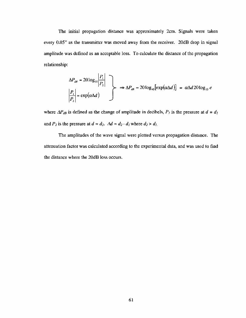
The initial propagation distance was approximately 2cm. Signals were taken

every 0.05" as the transmitter was moved away from the receiver. 20dB drop in signal

amplitude was defined as an acceptable loss. To calculate the distance of the propagation

relationship:

where APdB is defined as the change of amplitude in decibels, PI is the pressure at d = dl

and P2 is the pressure at d = d2. Ad = d2 - dl where d2 > dl.

The amplitudes of the wave signal were plotted versus propagation distance. The

attenuation factor was calculated according to the experimental data, and was used to find

the distance where the 20dB loss occurs.

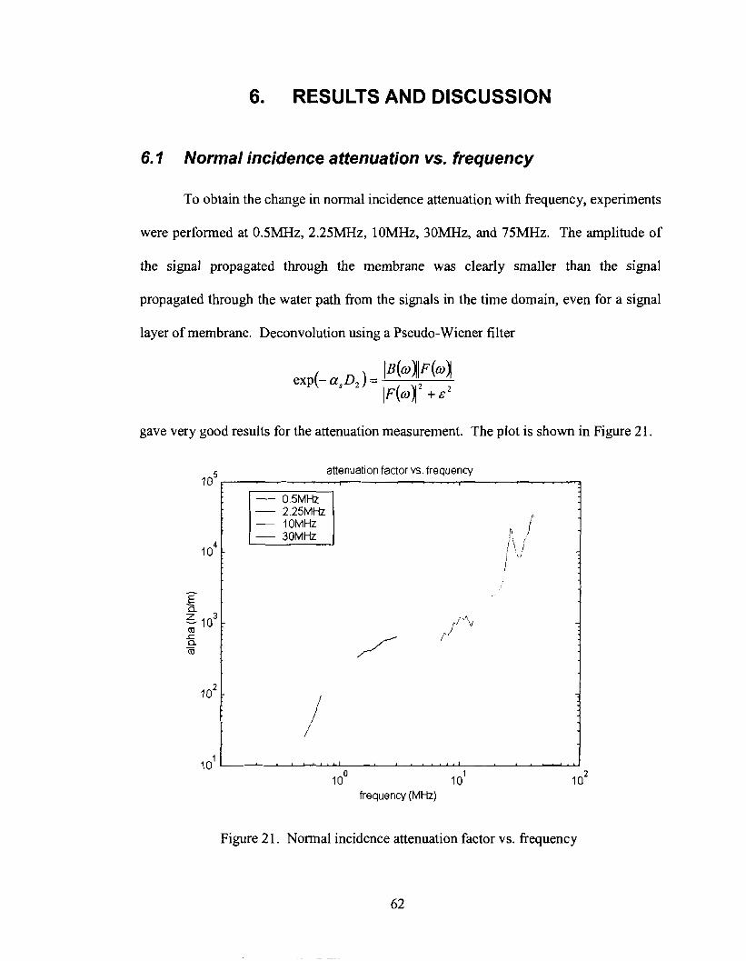
6. RESULTS AND DISCUSSION

6.7 Normal incidence attenuation vs. frequency

To obtain the change in normal incidence attenuation with frequency, experiments

were performed at OSMHz, 2.25MHz, lOMHz, 30MHz, and 75MHz. The amplitude of

the signal propagated through the membrane was clearly smaller than the signal

propagated through the water path from the signals in the time domain, even for a signal

layer of membrane. Deconvolution using a Pseudo-Wiener filter

gave very good results for the attenuation measurement. The plot is shown in Figure 2 1.

attenuation factor vs. frequency I o5

frequency (MHz)

Figure 21. Normal incidence attenuation factor vs. frequency

It is clear that the attenuation of the PVDF membrane increases with

frequency. The increase furthermore does not appear to be linear. It also does not

indicate what functional fit would be the best match to calculate the normal incident

attenuation of the PVDF membrane. However, no evidence shows that there is a global

peak of the attenuation curve. It also appears that at least one inflection point occurs in

the range considered

Since water is a highly attenuating medium for ultrasonic waves at high

frequencies, significant signal loss occurs in the signal from the 75MHz transducer

[Ramaswamy, 20021. The peak frequency of the signal from 75MHz transducer is

approximately 27MHz. Thus for the configuration used, information on the attenuation at

higher frequency is not analyzable.

Single frequency signals were used to check the result of deconvolution method.

The attenuation factors were calculated according to the equation:

Figure 22 gives the attenuation factors calculated by both deconvolution and

single frequency method. Though the values are not exactly the same, the results are

comparable.

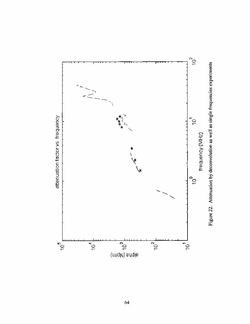
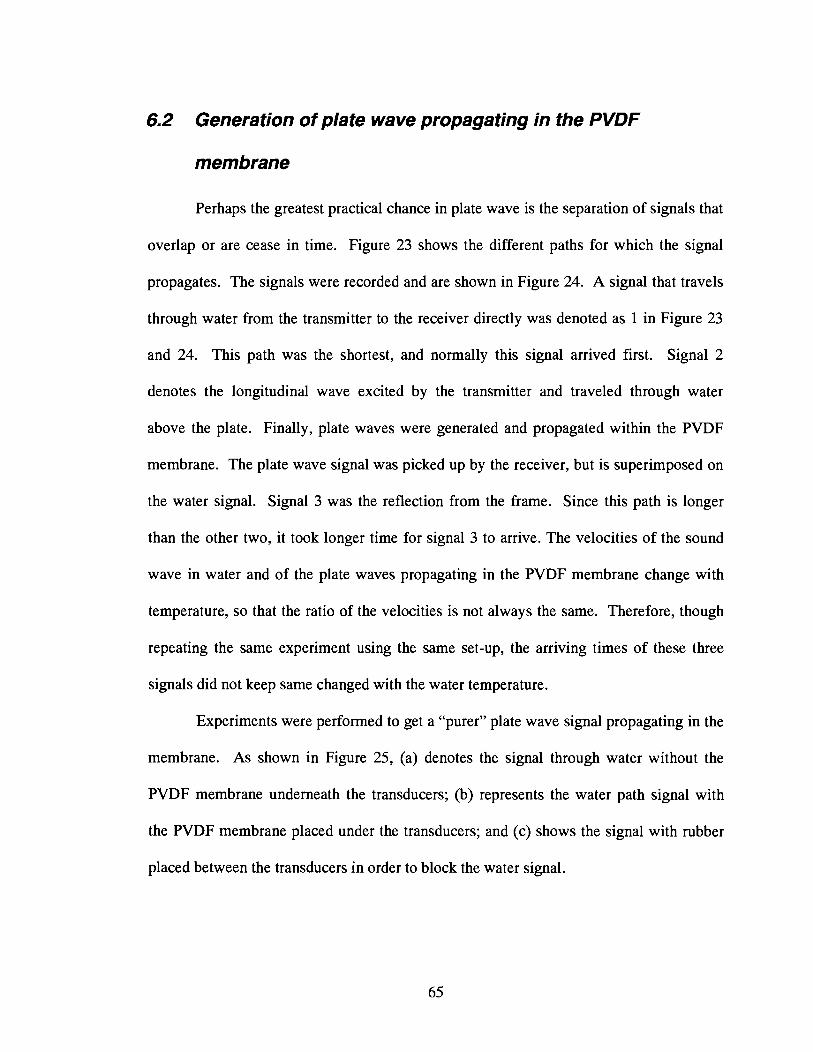
6.2 Generation of plate wave propagating in the PVDF

membrane

Perhaps the greatest practical chance in plate wave is the separation of signals that

overlap or are cease in time. Figure 23 shows the different paths for which the signal

propagates. The signals were recorded and are shown in Figure 24. A signal that travels

through water from the transmitter to the receiver directly was denoted as 1 in Figure 23

and 24. This path was the shortest, and normally this signal arrived first. Signal 2

denotes the longitudinal wave excited by the transmitter and traveled through water

above the plate. Finally, plate waves were generated and propagated within the PVDF

membrane. The plate wave signal was picked up by the receiver, but is superimposed on

the water signal. Signal 3 was the reflection from the frame. Since this path is longer

than the other two, it took longer time for signal 3 to arrive. The velocities of the sound

wave in water and of the plate waves propagating in the PVDF membrane change with

temperature, so that the ratio of the velocities is not always the same. Therefore, though

repeating the same experiment using the same set-up, the arriving times of these three

signals did not keep same changed with the water temperature.

Experiments were performed to get a "purer" plate wave signal propagating in the

membrane. As shown in Figure 25, (a) denotes the signal through water without the

PVDF membrane underneath the transducers; (b) represents the water path signal with

the PVDF membrane placed under the transducers; and (c) shows the signal with rubber

placed between the transducers in order to block the water signal.

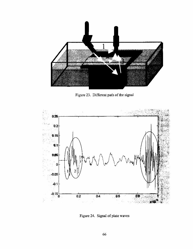
Figure 23. Different path of the signal

Figure 24. Signal of plate waves

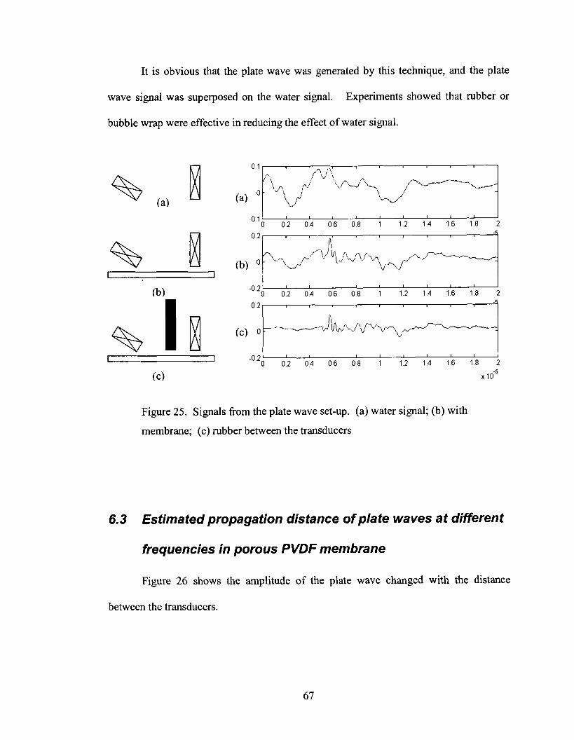
It is obvious that the plate wave was generated by this technique, and the plate

wave signal was superposed on the water signal. Experiments showed that rubber or

bubble wrap were effective in reducing the effect of water signal.

Figure 25. Signals from the plate wave set-up. (a) water signal; (b) with

membrane; (c) rubber between the transducers

6.3 Estimated propagation distance of plate waves at different

frequencies in porous PVDF membrane

Figure 2 6 shows the amplitude of the plate wave changed with the distance

between the transducers.

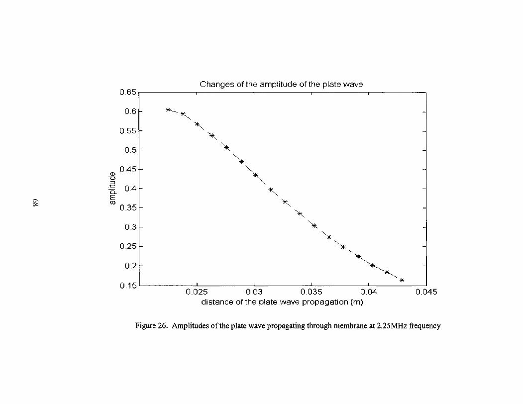
Changes of the amplitude of the plate wave 0.65 I I I I

Figure 26. Amplitudes of the plate wave propagating through membrane at 2.25MHz frequency

-

-

-

-

-

-

-

-

-

-

I I #

0 . 1 5 ~ I I

0.025 0 .03 0.035 0 .04 0.045 distance of the plate wave propagation (m)

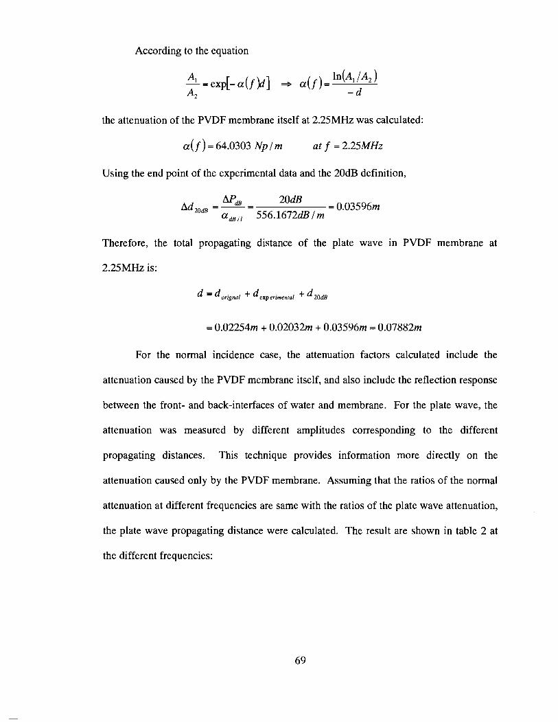
According to the equation

the attenuation of the PVDF membrane itself at 2.25MHz was calculated:

a ( f ) = 64.0303 Nplm at f = 2.25MH.z

Using the end point of the experimental data and the 20dB definition,

Therefore, the total propagating distance of the plate wave in PVDF membrane at

2.25MHz is:

= 0.02254m + 0.02032m + 0.03596m = 0.07882m

For the normal incidence case, the attenuation factors calculated include the

attenuation caused by the PVDF membrane itself, and also include the reflection response

between the front- and back-interfaces of water and membrane. For the plate wave, the

attenuation was measured by different amplitudes corresponding to the different

propagating distances. This technique provides information more directly on the

attenuation caused only by the PVDF membrane. Assuming that the ratios of the normal

attenuation at different frequencies are same with the ratios of the plate wave attenuation,

the plate wave propagating distance were calculated. The result are shown in table 2 at

the different frequencies:

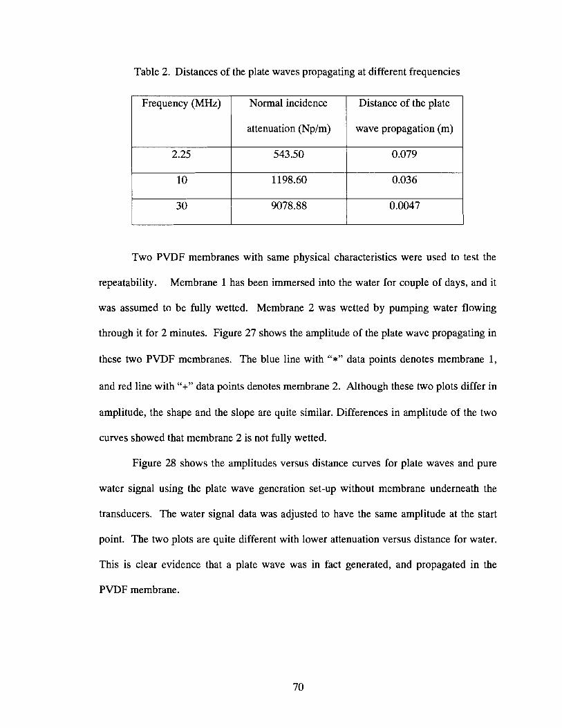
Table 2. Distances of the plate waves propagating at different frequencies

Two PVDF membranes with same physical characteristics were used to test the

repeatability. Membrane 1 has been immersed into the water for couple of days, and it

was assumed to be fully wetted. Membrane 2 was wetted by pumping water flowing

through it for 2 minutes. Figure 27 shows the amplitude of the plate wave propagating in

these two PVDF membranes. The blue line with "a" data points denotes membrane 1,

and red line with "+" data points denotes membrane 2. Although these two plots differ in

amplitude, the shape and the slope are quite similar. Differences in amplitude of the two

curves showed that membrane 2 is not fully wetted.

Figure 28 shows the amplitudes versus distance curves for plate waves and pure

water signal using the plate wave generation set-up without membrane underneath the

transducers. The water signal data was adjusted to have the same amplitude at the start

point. The two plots are quite different with lower attenuation versus distance for water.

This is clear evidence that a plate wave was in fact generated, and propagated in the

PVDF membrane.

Distance of the plate

wave propagation (m)

Frequency (MHz) Normal incidence

attenuation (Nplm)

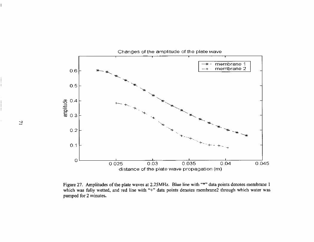
Changes of the amplitude of the plate wave

Figure 27. Amplitudes of the plate waves at 2.25MHz. Blue line with "*" data points denotes membrane 1 which was fully wetted, and red line with "+" data points denotes membrane2 through which water was pumped for 2 minutes.

-

-

-

d

-

-

-

I I I I

0.025 0 .03 0 .035 0 .04 0 .045 distance of the plate wave propagation (m)

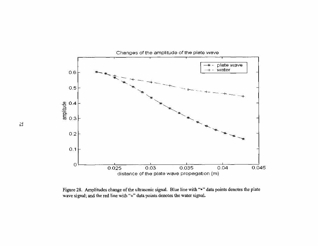
Changes of the amplitude of the plate wave I I 1 I

0.025 0 .03 0 .035 0 .04 0 .045 distance of the plate wave propagation (m)

Figure 28. Amplitudes change of the ultrasonic signal. Blue line with "*" data points denotes the plate wave signal; and the red line with "+" data points denotes the water signal.

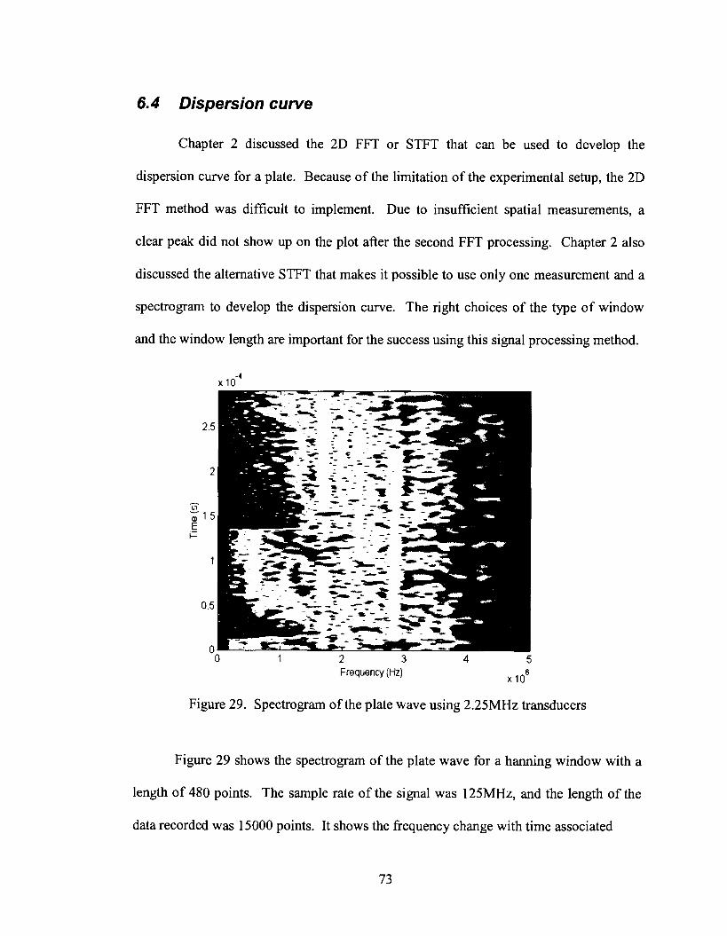
6.4 Dispersion curve

Chapter 2 discussed the 2D FFT or STFT that can be used to develop the

dispersion curve for a plate. Because of the limitation of the experimental setup, the 2D

FFT method was difficult to implement. Due to insufficient spatial measurements, a

clear peak did not show up on the plot after the second FFT processing. Chapter 2 also

discussed the alternative STFT that makes it possible to use only one measurement and a

spectrogram to develop the dispersion curve. The right choices of the type of window

and the window length are important for the success using this signal processing method.

0 1 2 3 4 5 Frequency (Hz)

x lo6

Figure 29. Spectrogram of the plate wave using 2.25MHz transducers

Figure 29 shows the spectrogram of the plate wave for a hanning window with a

length of 480 points. The sample rate of the signal was 125MHz, and the length of the

data recorded was 15000 points. It shows the frequency change with time associated

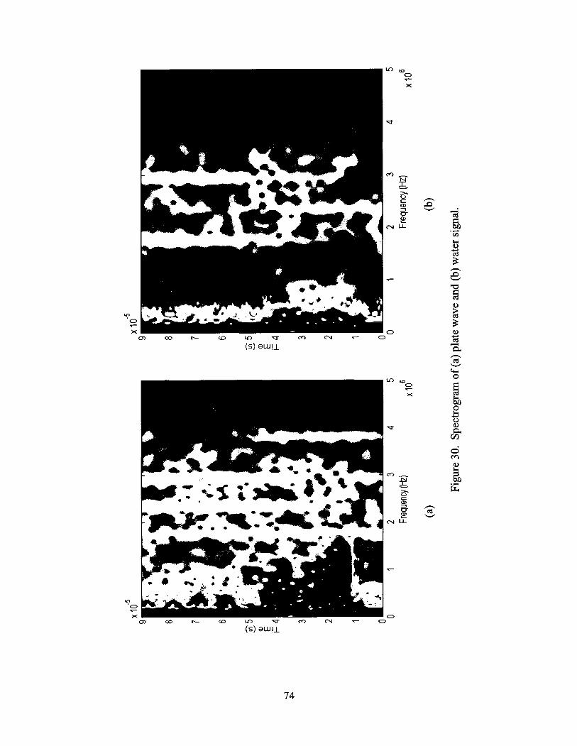
with a signal with dispersion. Figure 30 shows the spectrograms of the plate wave and

water signal in a short time period. The plate wave propagating through the PVDF

membrane is dispersive, and obviously different from the water signal.

It is difficult to determine how many and which modes propagate through the

PVDF membrane from the spectrogram. Theoretical calculation is needed at this point to

get more information about the modes.

6.5 Discussion: Expected area of membrane to be inspected

with plate waves

A transducer's sensitivity is affected by the beam diameter at the point of interest.

Figure 31 gives a graphical representation of the beam diameter.

Focal Zone

I I

-6dB beam diameter

Figure 31. Graphical representation of beam parameters

The -6dB beam diameter at the focus can be calculated with

BD(- 6dB) = 1 . 0 2 ~ ~ l p

or BD(- 6dB) = 0.2568DSF

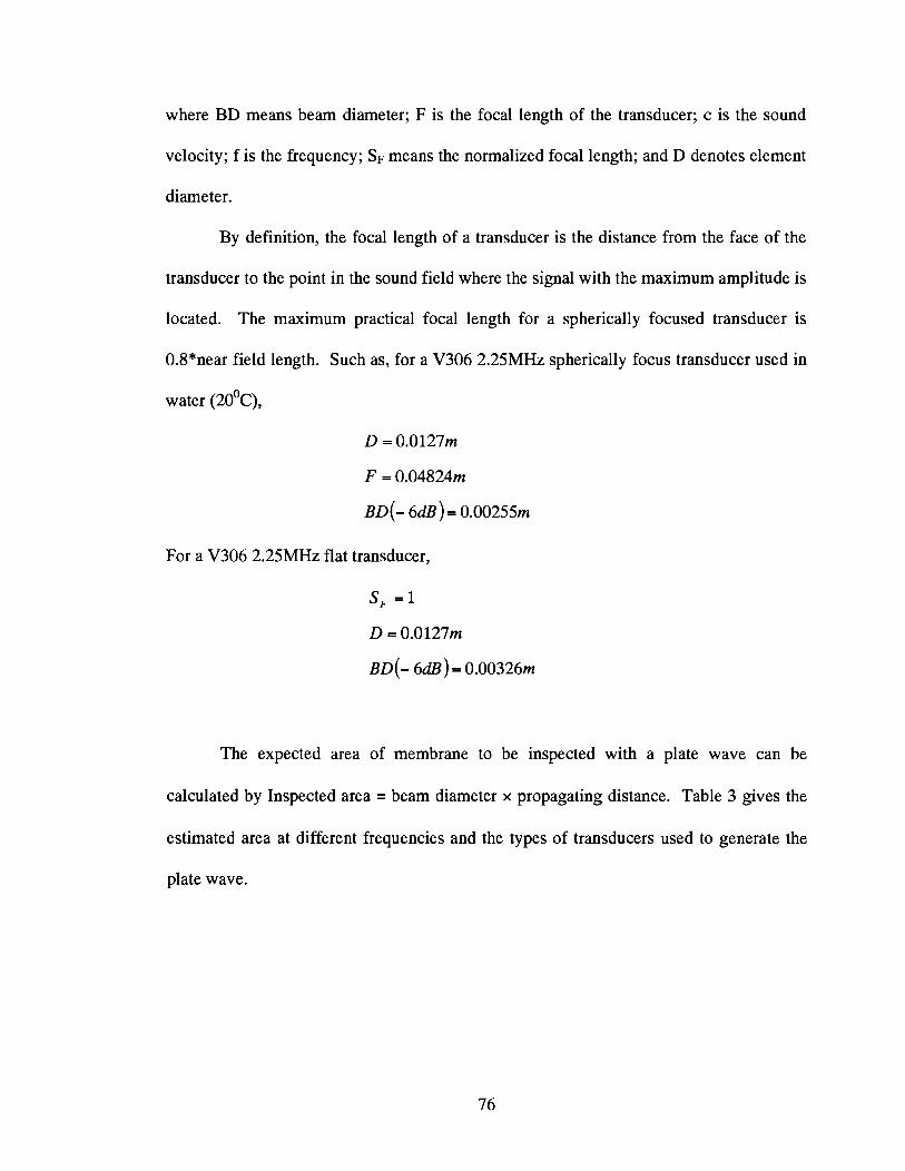
where BD means beam diameter; F is the focal length of the transducer; c is the sound

velocity; f is the frequency; SF means the normalized focal length; and D denotes element

diameter.

By definition, the focal length of a transducer is the distance from the face of the

transducer to the point in the sound field where the signal with the maximum amplitude is

located. The maximum practical focal length for a spherically focused transducer is

0.8*near field length. Such as, for a V306 2.25MHz spherically focus transducer used in

water (20°c),

For a V306 2.25MHz flat transducer,

The expected area of membrane to be inspected with a plate wave can be

calculated by Inspected area = beam diameter x propagating distance. Table 3 gives the

estimated area at different frequencies and the types of transducers used to generate the

plate wave.

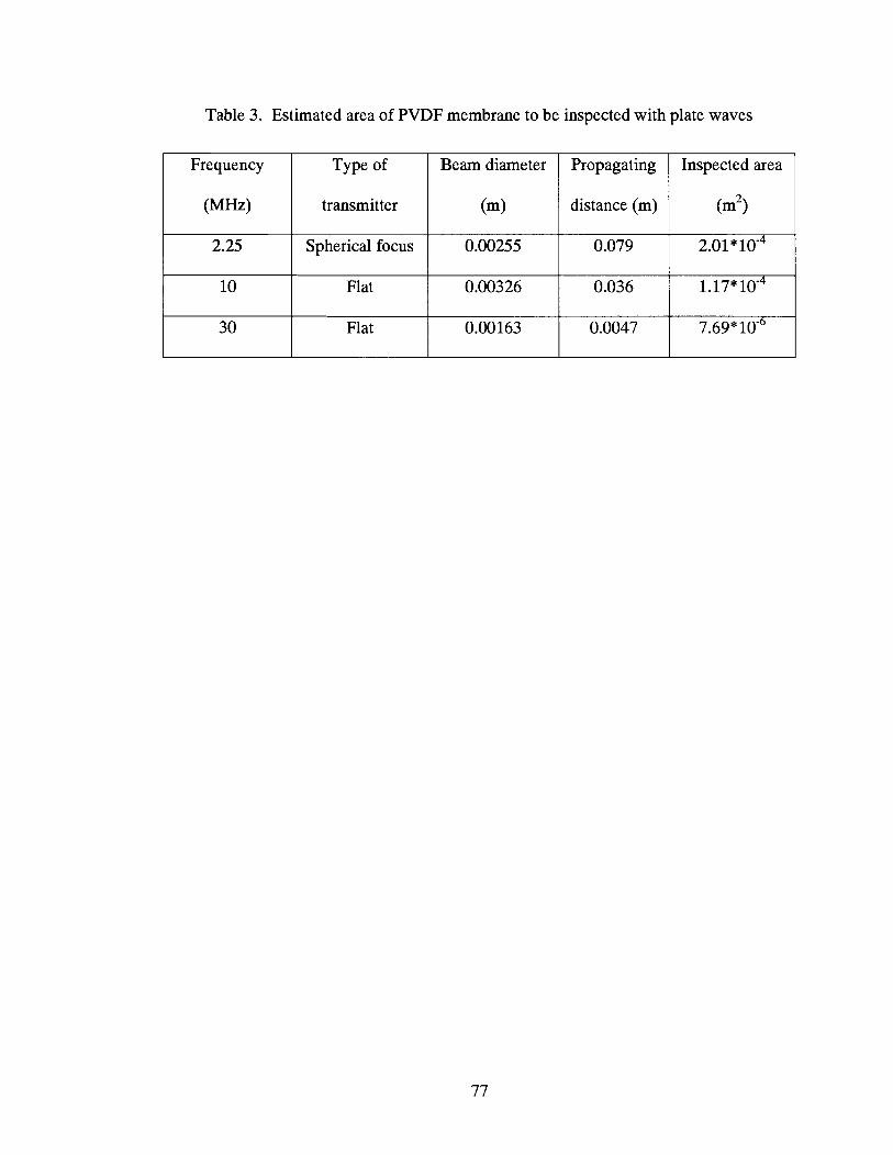
Table 3. Estimated area of PVDF membrane to be inspected with plate waves

Frequency

(MHz)

10 I Flat 1 0.00326 1 0.036 1 1.17*10-~

2.25

Type of

transmitter

Spherical focus

30

Beam diameter

(m)

0.00255

Flat

Propagating

distance (m)

Inspected area

(m2)

0.079

0.00163

2.01 *

0.0047 7.69*

CONCLUSIONS AND FUTURE WORK

An immersion method to measure the attenuation of membranes in the frequency

domain has been demonstrated. The approach is based on the deconvolution of a second

response signal. The attenuation of the PVDF membrane increases with frequency, and

does not appear linear. No evidence shows that there is a global peak of the attenuation

curve. There is at least one inflection point occurs in the range considered. A method

using a single frequency or narrow band excitation was performed to calibrate the

attenuation factor curve of the PVDF membrane.

A method was also developed to generate the ultrasonic plate wave, and

propagate it in the PVDF membrane. The potential propagating distances of the plate

waves at different frequencies were estimated, and the results show that the range of the

propagating distances is from 0.079m at 2.25MHz to 0.0047m at 30 MHz. The inspected

area of the membrane with a plate wave was also discussed in this work, and the

inspection ranged from 2.01cm2 at 2.25MHz to 7.69mm2 at 30MHz.

Finally, spectrograms of the plate wave were shown in this work. These

spectrograms showed the dispersive characteristics of the plate wave, but no conclusion

could be drawn at this point about the details of the wave modes.

Future work can be focused on two aspects. One is to identify the wave by a

numerical method and to further understand its behavior. Numerical methods can be

used to simulate the plate wave propagating in the membranes, and the dispersion curve

can be calculated. Further the numerical dispersion curve can be used to compare the

experimental spectrogram, and more information about the characteristics of the plate

wave and the mode will be drawn.

In this work, the plate waves were only observed at 2.25MHz frequency. More

experiments are expected at higher frequency, since a higher incident frequency would be

required in practice, so that smaller defects can be detected. Methods to decrease the

attenuation and increase the propagating distance at high frequency will be a very

important issue.

A suggestion to make this technique applicable to the on-line testing is to develop

a 3D surface plot, which has time, amplitude, and space axis. Because of the wrinkles of

the membrane itself, and wrinkles caused by the mounting frame or water flow, it will be

difficult to compare to a standard signal. A 3D surface plot however would be expected

to show more gradual changes caused by the wrinkles versus sharp variations which

would be caused by defects.

REFERENCES

Achenbach, J. D. 1984. Wavepropagation in elastic solids. New York: North-Holland Publishing Company.

Alderson, K. L., R. S. Webber, U. F. Mohammed, E. Murphy, and K. E. Evans. 1997. Experimental study of ultrasonic attenuation in microporous polyethylene. Appl. Acoust. 50(1): 23-33.

Alleyne, D., and P. Cawley. 1991. A two-dimensional Fourier transform method for the measurement of propagating multimode signals. J. Acoust. Soc. Am. 89(3): 1159- 1168.

Berryman, J. G. 1980. Confirmation of Biot's theory. Appl. Phys. Lett. 37(4): 382-384.

Berryman, J. G. 1981. Elastic wave propagation in fluid-saturated porous media. J. Acoust. Soc. Am. 69(2): 416-424.

Berryman, J. G. 1983. Dispersion of extensional waves in fluid-saturated porous cylinders at ultrasonic frequencies. J. Acoust. Soc. Am. 74(6): 1805-1812.

Berryman, J. G., and L. Thigpen. 1985. Effective constants for wave propagation through partially saturated porous media. Appl. Phys. Lett. 46(8): 722-724.

Billy, M. D., L. Adler, and G. Quentin. 1984. Measurements of backscattered leaky Lamb waves in plates. J. Acoust. Soc. Am. 75(3): 998-1001.

Biot, M. A. 1956. Theory of propagation of elastic waves in a fluid-saturated porous solid I. Low-frequency ranges. J. Acoust. Soc. Am. 28(2): 168-178.

Boyer, Howard E. et al. 1976. Metals Handbook: Nondestructive inspection and quality control. gth ed. llth Volume. Ohio: American Society for Metals.

Brown, R., and J. Korringa. 1975. On the dependence of the elastic properties of a porous rock on the compressibility of the pore fluid. Geophys. 40: 608-616.

Chimenti, D. E. 1997. Guided waves in plates and their use in materials characterization. Appl. Mech. Rev. 50(5): 247-284.

Chimenti, D. E., and S. I. Rokhlin. 1990. Relationship between leaky Lamb modes and reflection coefficient zeros for a fluid-coupled elastic layer. J. Acoust, Soc. Am. 88(3): 1603-1611.

Cohen, L. 1995. Time-Frequency Analysis. New Jersey: Prentice-Hall, Inc.

Corsaro, R. D., and L. H. Sperling. 1990. Sound and Vibration Damping with Polymers. Washington DC: American Chemical Society.

Dayal, V., and C. Afful. 1993. Plate wave measurement for material properties. NCA- Vo1.16/AMD-Vo1.172 of Dynamic Characterization ofAdvanced Materials. Edited by P . K. Raju, and R. F. Gibson. New York: The American Society of Mechanical Engineering.

Dayal, V., and V. K. Kinra. 1989. Leaky Lamb waves in an anisotropic plate. I: An exact solution and experiments. J. Acoust. Soc. Am. 85(6): 2268-2276.

Graff, K. F. 1991. Wave Motion in Elastic Solids. New York: Dover Publications, Inc.

Hartmann, B. 1980. Methods of experimentalphysics. Vol. 16c: 59-90. New York: Academic Press. Inc.

Hickey, C. J., and J. M. Sabatier. 1997. Measurements of two types of dilatational waves in an air-filled unconsolidated sand. J. Acoust. Soc. Am. 102(1): 128-136.

Johnson, D. L., J. Koplik, and R. Dashen. 1987. Theory of dynamic permeability and tortuosity in fluid-saturated porous media. J. Fluid Mech. 176: 379-402.

Johnson, D. L., D. L. Hemmick, and H. Kojima. 1994. Probing porous media with first and second sound. I. Dynamic permeability. J. Appl. Phys. 76(1): 104-114.

Johnson, D. L., T. J. Plona, and H. Kojima. 1994. Probing porous media with first and second sound. 11. Acoustic properties of water-saturated porous media. J. Appl. Phys. 76(1): 115-125.

Jones, D. I. G. 2001. Handbook of viscoelastic vibration damping. Chichester, England: John Wiley & Sons, Ltd.

Khulbe, K. C., and T. Matsuura. 2000. Characterization of synthenic membranes by Raman spectroscopy, electron spin resonance, and atomic force microscopy. Polymer 41: 1917-1935.

Kim, K. J., A. G. Fane, R. Ben Aim, M. G. Liu, G. Jonsson, I. C. Tessaro, A. P. Broek, and D. Bargeman. 1994. A comparative study of techniques used for porous membrane characterization: pore characterization. J. Membrane Science 87: 35- 46.

Kim, Y. H., S. J. Song, and S. D. Kwon. 2002. Measurement of phase velocity dispersion curves and group velocities in a plate using leaky Lamb waves. National Seminar of ISNT Chennai: 5. - 7.12.

Kools, W. F. C., S. Konagurthu, A. R. Greenburg, L. J. Bond, W. B. Krantz, Th. V. D. Boomgaard, and H. Strathrnann. 1998. Use of Ultrasonic Time-Domain Reflectometry for Real-Time Measurement of Thickness Changes During Evaporative Casting of Polymeric Films. J. Applied Polymer Science. 69: 2013- 2019.

Krautkramer, J., and H. Krautkramer. 1983. Ultrasonic Testing of Materials. Berlin: Springer-Verlag.

Li, J., and R. D. Sanderson. 2002. In situ measurement of particle deposition and its removal in microfiltration by ultrasonic time-domain reflectometry. Desalination 46: 169-175.

Lloyd, D. R. 1985. Materials Science of Synthetic Membranes (ACS symposium series 269). Washington DC: American Chemical Society.

Mairal, A. P., A. R. Greenburg, W. B. Krantz, and L. J. Bond. 1999. Real-time measurement of inorganic fouling of RO desalination membrane using ultrasonic time-domain reflectometry. J. Membrane Science 159: 185-196.

Mairal, A. P., A. R. Greenburg, and W. B. Krantz. 2000. Investigation of membrane fouling and cleaning using ultrasonic time-domain reflectometry. Desalination 130: 45-60.

Matsuura, T. 1994. Synthetic Membranes and Membrane Separation Processes. Boca Raton, Florida: CRC Press.

Mavko, G., T. Mukerji, and J. Dvorkin. 1998. The Rock Physics Handbook: Tools for Seismic Analysis in Porous Media. Cambridge: Cambridge University Press.

Mohr, C. M., D. E. Engelgan, S. A. Leeper, and B. L. Charboneau. 1989. Membrane Applications and Research in Food Processing. New Jersey: Noyes Data Corporation.

Nayfeh, A.H., and P.B. Nagy. 1997. Excess attenuation of leaky Lamb waves due to viscous fluid loading. J. Acoust. Soc. Am. lOl(5): 2649-2658.

Niethammer, M. 1999. Application of Time Frequency Representations to Characterize Ultrasonic Signal. Master's thesis, Georgia Institute of Technology.

Niethammer, M., and L. J. Jacobs. 2000. Time-frequency representation of Lamb waves using the reassigned spectrogram. J. Acoust. Soc. Am. 107(5): L19-L24.

Niethammer, M., L. J. Jacobs, J. Qu, and J. Jarzynski. 2001. Time-frequency representation of Lamb wave. J. Acoust. Soc. Am. 109(5): 1841-1847.

Panakkal, J. P. 1996. Longitudinal ultrasonic velocity as a predictor of material properties of porous materials. Trends in NDE Science & Technology 4: 2279- 2282.

Parra, J. O., and P. C. Xu. 1994. Dispersion and attenuation of acoustic guided waves in layered fluid-filled porous media. J. Acoust. Soc. Am. 95(1): 91-98.

Peterson, M. L. 1994. A Signal Processing Technique for Measurement of Multi-Mode Waveguide Signals: An Application to Monitoring of Reaction Bonding in Silicon Nitride. Research in Nondestructive Evaluation 5: 239-256.

Peterson, R. A., A. R. Greenburg, L. J. Bond, and W. B. Krantz. 1998. Use of Ultrasonic TDR for real-time noninvasive measurement of compressive strain during membrane compaction. Desalination 116: 115-122.

Pinnan, I., and B. D. Freeman. 2000. Membrane Formations and Modification. Washington DC: American Chemical Society, Oxford University Press.

Plona, T. J. 1980. Observation of a second bulk compressional wave in a porous medium at ultrasonic frequencies. Appl. Phys. Lett. 36(4): 259-261.

Plona, T. J., and D. L. Johnson. 1980. Experimental study of the bulk compressional modes in water-saturated porous structures. Ultrasonic Symposium 1980: 868- 872.

Puckett, A. D. 2000. Fidelity of a Finite Element Model for Longitudinal Wave Propagation in Thick Cylindrical Wave Guides. Master's thesis, Colorado State University.

Ramaswamy, S. 2002. Development of an Ultrasonic Technique for the Non-Invasive Characterization of Membrane Morphology. Ph.D. dissertation, University of Colorado.

Redwood, M. 1960. Mechanical Waveguides. Bristol: Pergamon Press.

Rose, J. L. 1999. Ultrasonic Waves in Solid Media. Cambridge: Cambridge University Press.

Schrnerr, L. W. Jr. 1998. Fundamentals of Ultrasonic nondestructive evaluation - A modeling approach. New York and London: Plenum Press.

Scott, K. 1995. Handbook of Industrial Membranes. 1st Edition. Oxford: Elsevier Advanced Technology.

Seale, M. D., B. T. Smith, W. H. Prosser, and J. E. Masters. 1994. Lamb Wave Response of Fatigued Composite Samples. Vol. 13B: 1261-1266 of Review of Progress in QNDE. Edited by D. 0. Thompson and D. E. Chimenti. New York: Plenum Press,

Stoll, R. D. 1977. Acoustic waves in ocean sediments. Geophysics 42: 715-725.

Stoll, R. D. 1980. Theoretical aspects of sound transmission in sediments. J. Acoust. Soc. Am. 68(5): 1341-1350.

Wu, K., Q. Xue, and L. Adler. 1990. Reflection and transmission of elastic waves from a fluid-saturated porous solid boundary. J. Acoust. Soc. Am. 87(6): 2349-2358.

Xu, P. C., K. E. Lindenschrnidt, and S. A. Meguid. 1993. A new high-frequency analysis of coatings using leaky Lamb waves. J. Acoust. Soc. Am. 94(5): 2954- 2962.

APPENDICES

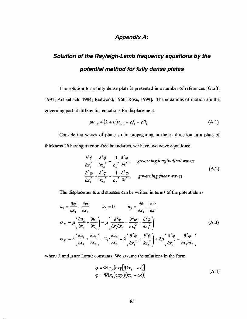
Appendix A:

Solution of the Rayleigh-Lamb frequency equations by the

potential method for fully dense plates

The solution for a fully dense plate is presented in a number of references [Graff,

1991; Achenbach, 1984; Redwood, 1960; Rose, 19991. The equations of motion are the

governing partial differential equations for displacement.

Considering waves of plane strain propagating in the XI direction in a plate of

thickness 2h having traction-free boundaries, we have two wave equations:

a2$ a2$ 1 a2$ -+-=-- 2 2 , governing longitudinal waves

ax, ax, cL2 at2

a2cp a2cp 1 a2cp ( A 4

-+-=-- 2 2 , governing shear waves ax, ax, C, at2

The displacements and stresses can be written in terms of the potentials as

a4 acp U1 =- +- u2 - 0 a$ acp

axl ax, U3 =--- ax, ax,

8 x 1 8 ~ ~ ax12 ax,

where A. and p are Lame constants. We assume the solutions in the form

4 = ~ ( x , )exp[i(bl - at)]

cp = Y (x, )exp[i(bl - at)]

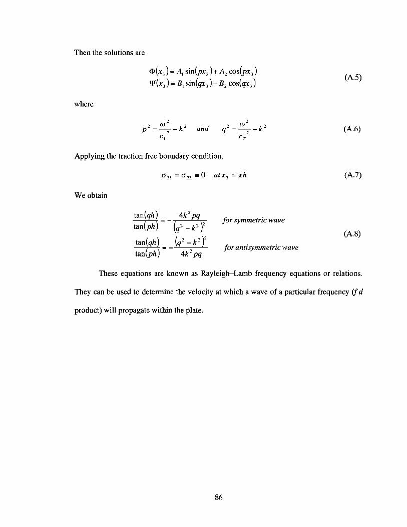
Then the solutions are

where

o2 2 o2 p2 =,-k2 and q =--k2 2

C L C T

Applying the traction free boundary condition,

o,, = o,, I 0 a tx , = +h

We obtain

tan(qh ) 4k ' pq for symmetric wave tan(ph) = - (q2 - k2 f

tan(qh) (q2 - k 2 Y (A.8)

for antisymmetric wave ta&h) = - 4k2pq

These equations are known as Rayleigh-Lamb frequency equations or relations.

They can be used to determine the velocity at which a wave of a particular frequency ( f d

product) will propagate within the plate.

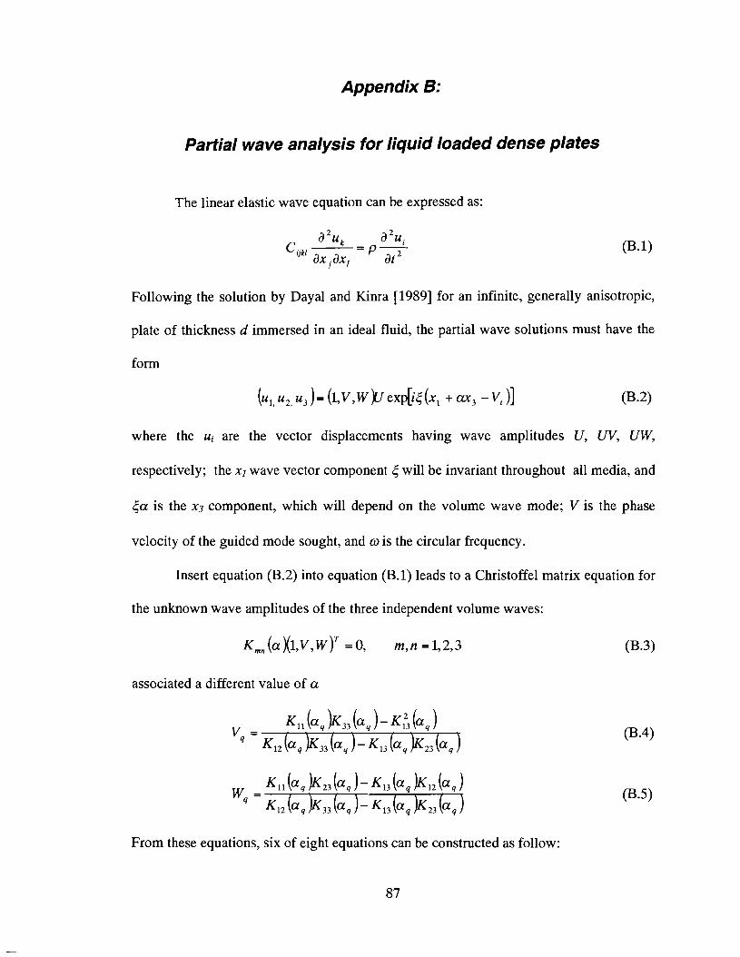
Appendix B:

Partial wave analysis for liquid loaded dense plates

The linear elastic wave equation can be expressed as:

a2uk a2ui -P- C,, - - ax, ax, at2

Following the solution by Dayal and Kinra [I9891 for an infinite, generally anisotropic,

plate of thickness d immersed in an ideal fluid, the partial wave solutions must have the

form

(.I, u2, u3 )= b,v,w)LI exp[i~(x, + a 3 -V, I1 (B.2)

where the ui are the vector displacements having wave amplitudes U, W, UW,

respectively; the xl wave vector component 5 will be invariant throughout all media, and

5a is the x3 component, which will depend on the volume wave mode; V is the phase

velocity of the guided mode sought, and w is the circular frequency.

Insert equation (B.2) into equation (B.l) leads to a Christoffel matrix equation for

the unknown wave amplitudes of the three independent volume waves:

K , , ( ~ ) ( ~ , v , w ) ~ =0, m,n=l ,2 ,3

associated a different value of a

wq = &I (aq k 2 3 b q )- K~~ (aq k12 (aq ) ~ 1 2 (aq k33 (aq (aq 1 ~ 2 3 (aq 1

From these equations, six of eight equations can be constructed as follow:

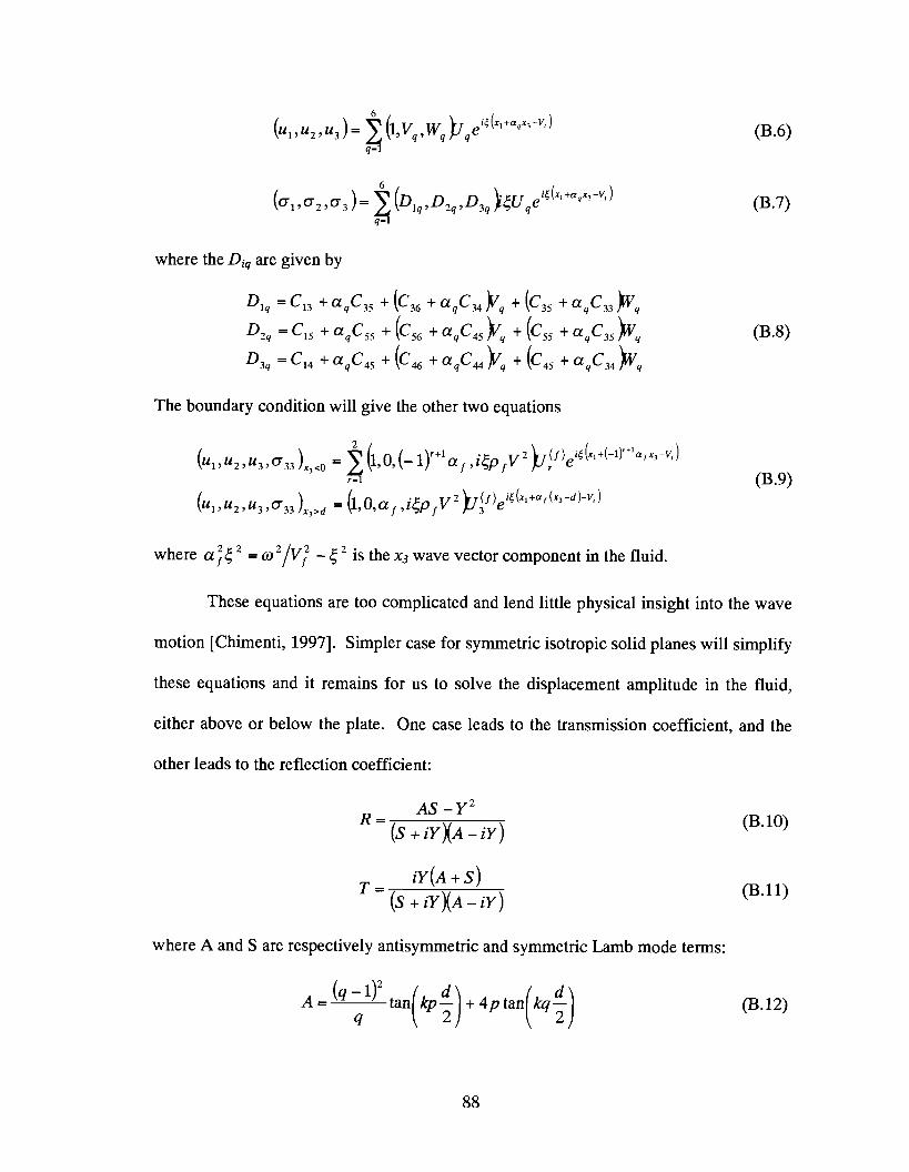
where the Di, are given by

The boundary condition will give the other two equations

where a ;g = a '/v; - 4 is the x3 wave vector component in the fluid.

These equations are too complicated and lend little physical insight into the wave

motion [Chimenti, 19971. Simpler case for symmetric isotropic solid planes will simplify

these equations and it remains for us to solve the displacement amplitude in the fluid,

either above or below the plate. One case leads to the transmission coefficient, and the

other leads to the reflection coefficient:

where A and S are respectively antisymmetric and symmetric Lamb mode terms:

A = (q-1)2 tan kp- +4ptan kq- 4 ( : ( :I

(B. 10)

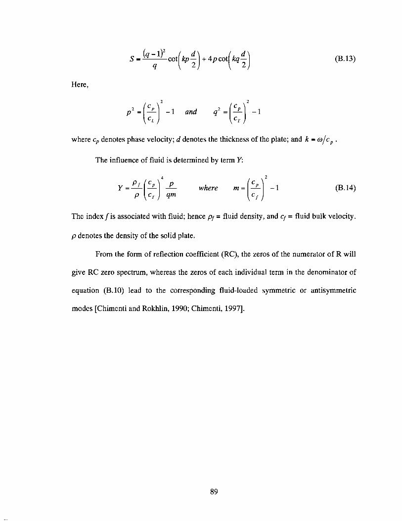
(B. 13)

Here,

where c, denotes phase velocity; d denotes the thickness of the plate; and k = w/c, .

The influence of fluid is determined by term Y:

The index f is associated with fluid; hence pf = fluid density, and cf = fluid bulk velocity.

p denotes the density of the solid plate.

From the form of reflection coefficient (RC), the zeros of the numerator of R will

give RC zero spectrum, whereas the zeros of each individual term in the denominator of

equation (B.lO) lead to the corresponding fluid-loaded symmetric or antisymmetric

modes [Chimenti and Rokhlin, 1990; Chimenti, 19971.

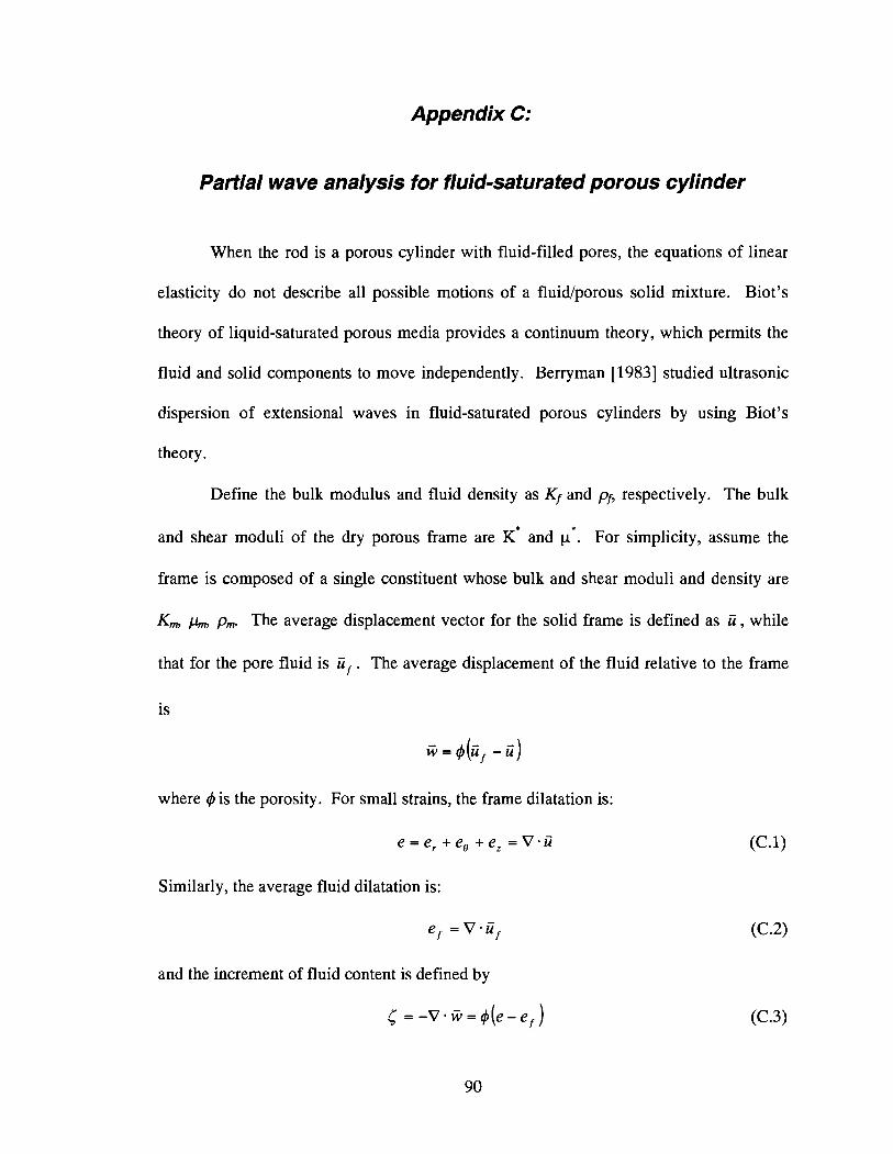
Appendix C:

Partial wave analysis for fluid-saturated porous cylinder

When the rod is a porous cylinder with fluid-filled pores, the equations of linear

elasticity do not describe all possible motions of a fluidlporous solid mixture. Biot's

theory of liquid-saturated porous media provides a continuum theory, which permits the

fluid and solid components to move independently. Berryman [I9831 studied ultrasonic

dispersion of extensional waves in fluid-saturated porous cylinders by using Biot's

theory.

Define the bulk modulus and fluid density as Kf and pf, respectively. The bulk

and shear moduli of the dry porous frame are K* and For simplicity, assume the

frame is composed of a single constituent whose bulk and shear moduli and density are

Km) pm) pm. The average displacement vector for the solid frame is defined as ii, while

that for the pore fluid is ii, . The average displacement of the fluid relative to the frame

is

+&if - 6 )

where 4 is the porosity. For small strains, the frame dilatation is:

e = e , +e, +e, =V.Z

Similarly, the average fluid dilatation is:

e , = V.iif

and the increment of fluid content is defined by

6 = - v . ~ = $ ( e - e , )

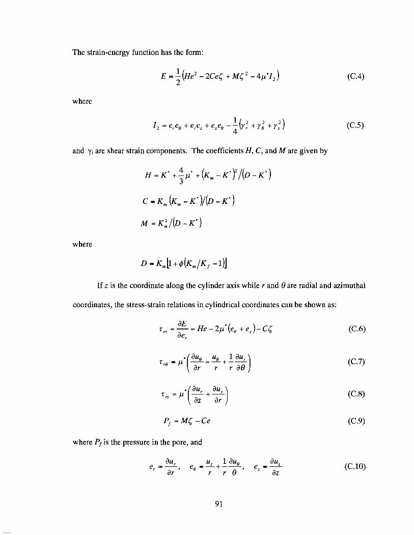
The strain-energy function has the form:

where

and yi are shear strain components. The coefficients H, C, and M are given by

If z is the coordinate along the cylinder axis while r and 8 are radial and azimuthal

coordinates, the stress-strain relations in cylindrical coordinates can be shown as:

P, = M< -Ce

where Pf is the pressure in the pore, and

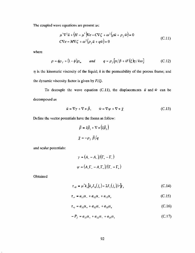
The coupled wave equations are present as:

p*v2ii + (H - p * k e - m < + 0 2 ( p i i + p , ~ ) = 0 (C. 11)

m e - m < + 0 2 ( p f i i + q ~ ) = 0

q is the kinematic viscosity of the liquid; k is the permeability of the porous frame; and

the dynamic viscosity factor is given by F ( Y .

To decouple the wave equation (C.11), the displacements ii and G can be

decomposed as

i i = v y + v x p , i+=vl ,U+vxa (C.13)

Define the vector potentials have the forms as follow:

p = i p , + v x (la2)

a = -P , 814

Obtained

(C. 14)

(C. 15)

(C.16)

(C. 17)

where k: = o2 (p - p; /q)p* ; Jo is the zero-order Bessel function of the first kind; and

the coefficients a,, as, and ys are constants to be determined from the boundary

conditions.

When the surface pores are open, the appropriate boundary conditions for

extensional waves are

the result will be given by

(C. 20)

When the surface pores are closed, the boundary conditions are

the result is given by

(C. 22)

BIOGRAPHY OF THE AUTHOR

Lin Lin was born in Dalian, China on January 15'~, 1972, and was raised in

Beijing, China. She attended Beijing Polytechnic University (which changed name into

Beijing University of Technology at 2001) and graduated in 1994 with a Bachelor's

degree in Thermal Energy Engineering. She worked as an assistant professor in the

Thermal Energy Engineering Department, and then in College of Environmental and

Energy Engineering at Beijing Polytechnic University. She came to University of Maine

to obtain a Master of Science degree in Mechanical Engineering in August 2001. She

joined the Mechanical Engineering graduate program as a teaching assistant and research

assistant.

Lin is a candidate for the Master of Science degree in Mechanical Engineering

from The University of Maine in August, 2003.