Embed Size (px)
Citation preview
HAL Id: hal-01193689https://hal.archives-ouvertes.fr/hal-01193689
Submitted on 6 Jun 2020
HAL is a multi-disciplinary open accessarchive for the deposit and dissemination of sci-entific research documents, whether they are pub-lished or not. The documents may come fromteaching and research institutions in France orabroad, or from public or private research centers.
L’archive ouverte pluridisciplinaire HAL, estdestinée au dépôt et à la diffusion de documentsscientifiques de niveau recherche, publiés ou non,émanant des établissements d’enseignement et derecherche français ou étrangers, des laboratoirespublics ou privés.
On the genetic interpretation of Between-Group PCAon SNP data
Denis Laloë, Mathieu Gautier
To cite this version:Denis Laloë, Mathieu Gautier. On the genetic interpretation of Between-Group PCA on SNP data.[Research Report] HAL : hal-00661214, version 1, auto-saisine. 2012, 23 p. �hal-01193689�
- 1 -
On the Genetic interpretation of Between-Group PCA on SNP data
Denis Laloë *1, Mathieu Gautier1,2
1 INRA, UMR 1313 de Génétique Animale et Biologie Intégrative, 78350 Jouy-en-Josas,
France.
2 INRA, UMR CBGP (INRA/IRD/Cirad/Montpellier SupAgro), Campus international de
Baillarguet, CS 30016, F-34988 Montferrier-sur-Lez cedex, France.
*Corresponding author
Email addresses:
DL : [email protected]
hal-0
0661
214,
ver
sion
1 -
18 J
an 2
012
- 2 -
Abstract Background Principal Components Analysis is a standard and computationally efficient method to explore
large SNP data sets. We propose in this study additional interpretations of PCA results about
the characterization of population genetic structure when dealing with SNP data. In particular,
we evaluate how SNP typological values obtained from PCA are related to F-statistics and
may help to identify footprints of selection.
Results We show that a normed PCA on biallelic SNP haplotypes is equivalent to a Multiple
Correspondence Analysis and to a PCA on the r correlation matrix, where r represent the
signed square root of the r2 linkage disequilibrium measure. Each resulting principal
component describes a typology and provides a measure of the underlying SNP contributions
which may further be interpreted in terms of correlation ratio and variance reduction. In
addition, PCA can be partitioned into sub-analyses (between-group, within-group). Between-
group PCA maximises the variance between groups and delivers principal components with
maximum FST. Only per-group allele frequencies and relative frequencies are needed to
compute between-group PCA. Finally, chromosomal regions containing SNPs with high
contributions may be interpreted as footprints of selection. As an illustration of the approach
we analyzed human chromosome 2 haplotypes sampled from three HapMap populations
(from African, Asian and European origin). We showed that SNPs within or close to EDAR
and LCT genes exhibit the highest typological values, in agreement with previous studies.
Conclusions When applied to biallelic SNP data, our PCA based proposed approach enables to describe the
genetic structuring of populations and to quantify for each typology the contributions of SNPs
by FST statistics. Taking into account spatial dependences of SNPs allows in turn to identify
hal-0
0661
214,
ver
sion
1 -
18 J
an 2
012
- 3 -
genomic regions contributing to the structuring of populations which might be interpreted as
footprints of selection. Finally, this approach was proven computationally efficient since it
can handle data including several hundreds of thousands SNPs within less than one hour on a
standard computer.
Background The availability of large numbers of SNPs uniformly distributed across the genome has
provided opportunities to refine the analysis of population structuring of genetic diversity.
The most commonly used methods are either model-based such as unsupervised hierarchical
clustering approach [1] or exploratory such as principal component analysis (PCA) [2-6].
Unsupervised hierarchical clustering approaches have been widely used in population
genetics studies because of the detailed information they provide on group membership and
individual admixture. However these model-based approaches tend to be computationally
intensive and are in practice not suited to the large numbers of markers present in genome-
wide data sets, even if new implementations are making the computational aspect less of a
problem [7-9]. In that context, PCA and related descriptive methods are especially appealing
since they are far less computationally demanding than other methods [3, 5]. PCA has been
used to treat large SNP datasets, especially in human (e.g. [10-13]), but also more recently in
cattle [14-16]. PCA has also been proposed to assess the extent of Linkage Disequilibrium
(LD) groups and to identify sets of group tagging SNPs over the genome [17, 18]. This latter
PCA is performed on the matrix of SNP-pairwise ∆ measures, also know as r, and
corresponding to the signed square root of the r2 LD measure [19]. More generally, whether
the focus is on variables (i.e. SNPs) or individuals, PCA may address two different questions
either relative to the relationships among SNPs or the genetic structuring of populations. Such
double functionality has been formalized through the duality diagram theory [20, 21].
hal-0
0661
214,
ver
sion
1 -
18 J
an 2
012
- 4 -
Studies focusing on relationships among markers mainly concentrate on two objectives. First,
PCA was proven powerful to reduce the complexity of the data sets, thereby facilitating data
visualisation and storage requirements [22], in particular via some extensions such as sparse
PCA, Lasso and Elastic Net [23, 24]. Paschou and collaborators [25] demonstrated that small
subsets of PCA based selected SNPs succeeded in assigning individuals to particular
populations. Hence, the number of SNPs for ancestry inference could be successfully reduced
to less than 0.1% while retaining close to 100% accuracy in the Human Genome Diversity
Panel data set [26]. Second, PCA and related methods provide measures of contribution of
markers to the genetic structuring of populations [4, 27]. When combined to a discriminant
analysis, as first proposed by [28], PCA also allows to measure the contributions of individual
alleles to the discrimination between populations [29].
Our study is in line with this second objective and capitalizes on the features of biallelic SNP
data in subdivided populations to propose new interpretations of PCA from both a statistical
and a genetic point of view. From a statistical point of view, we show that the equivalence
between PCA (when applied to dichotomous factors) and multiple correspondence analysis
(MCoA), the method of reference to deal with multiple contingency tables [30], leads to
appealing properties. From a genetic point of view, we show that the SNP squared scores
provided by the between-population PCA are estimators of FST. They may further be
interpreted with respect to the corresponding population substructure to identify putative
footprints of selection [31]. For the sake of an illustration, we finally analyzed a publicly
available and well studied human haplotype data set.
Results Haplotype-based PCA A detailed presentation of PCA can be found, for instance, in [32] and we just present herein
essential features of our method when applied to SNP haplotypes. Let X={xij} be a matrix
hal-0
0661
214,
ver
sion
1 -
18 J
an 2
012

- 5 -
with n rows (haplotypes) and p columns (SNPs). Since only biallelic SNPs are considered,
each entry of X is a binary indicator variable corresponding to one of the two alleles such as:
1 if the allele of SNP of the haplotype is the first allele
=0 if the allele of SNP of the haplotype is the second allele
ij
j ix j i
=
, Standardization of X leads to the matrix m( )
[ ]sd( )
jij
ij j
x xz
x −
= =
Z where m(xj) and sd(xj)=
(1 )j jp p− (where pj is the allele frequency of SNP j) are the mean and the standard
deviation for the j-th column of X. A normed PCA is a PCA on standardized variables (i.e.
Z).
It is worth noting that, with these notations, the LD measure ∆ between two SNPs j and k is
equal to the correlation between the jth and kth columns of X. Hence, the (symetric) matrix
Z’Z/n corresponds to the LD matrix based on the ∆ measure. [18].
According to the duality diagram theory [20], the PCA of Z is summarized by the triplet <Z,
Q, D>, where Q =Ip and D = In /n are metric matrices weighting the columns and the rows of
Z, respectively. The PCA is performed indifferently by the eigendecomposition of either
Z’DZQ=Z’Z/n (representation of individuals (haplotypes) in the SNPs hyperspace) or its
transpose ZQZ’D=ZZ’/n (representation of variables (SNPs) in the individual hyperspace).
Both decompositions produce the same set of eigenvalues, the number of which equals the
rank of Z’Z/n, say r. The eigendecomposition of Z’Z/n results in a set of eigenvectors called
principal components, which are linear combinations of the original SNPs. Conversely, the
eigendecomposition of ZZ’/n results in a set of eigenvectors called principal axes, which are
linear combinations of the original haplotypes. Transition formulae enable to move easily
from one set of eigenvectors to the other set. The scores of a haplotype is the projection of the
corresponding X row onto the principal components. Correspondingly, the scores of a SNP is
the projection of the corresponding X column onto the principal axes. Let cij be the score of
hal-0
0661
214,
ver
sion
1 -
18 J
an 2
012
- 6 -
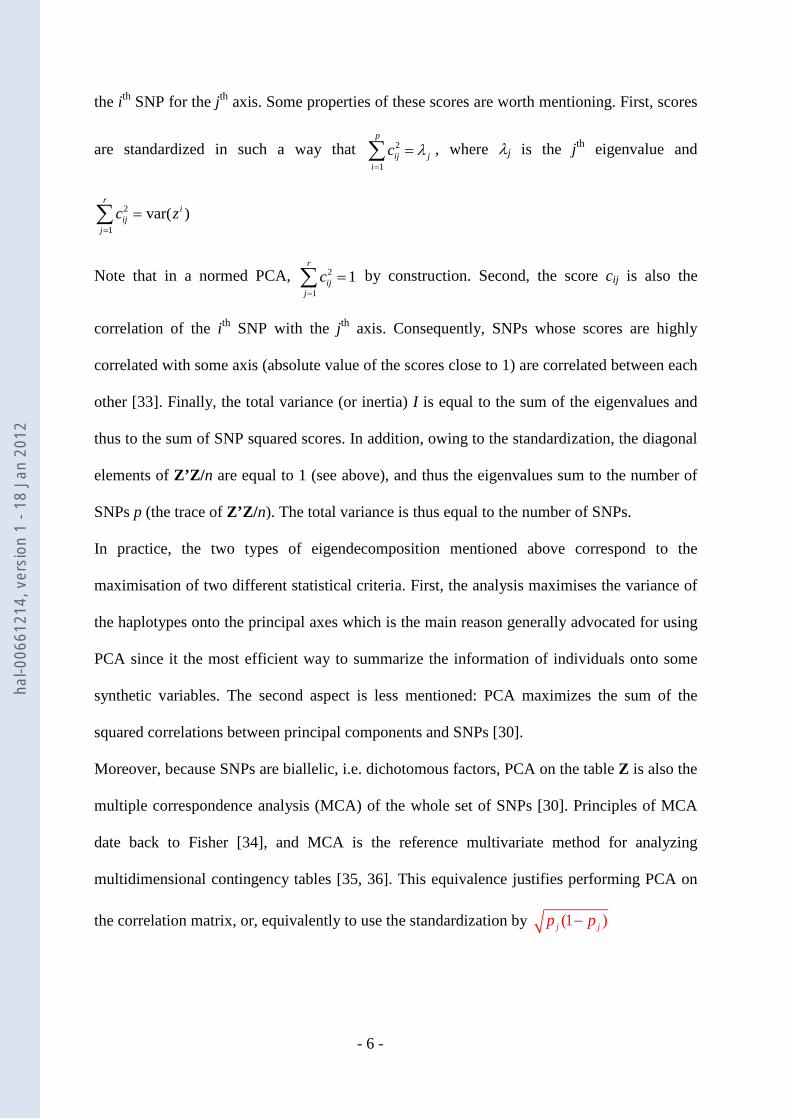
the ith SNP for the jth axis. Some properties of these scores are worth mentioning. First, scores
are standardized in such a way that 2
1
p
ij ji
c λ=
=∑ , where λj is the jth eigenvalue and
2
1var( )
ri
ijj
c z=
=∑
Note that in a normed PCA, 2
11
r
ijj
c=
=∑ by construction. Second, the score cij is also the
correlation of the ith SNP with the jth axis. Consequently, SNPs whose scores are highly
correlated with some axis (absolute value of the scores close to 1) are correlated between each
other [33]. Finally, the total variance (or inertia) I is equal to the sum of the eigenvalues and
thus to the sum of SNP squared scores. In addition, owing to the standardization, the diagonal
elements of Z’Z/n are equal to 1 (see above), and thus the eigenvalues sum to the number of
SNPs p (the trace of Z’Z/n). The total variance is thus equal to the number of SNPs.
In practice, the two types of eigendecomposition mentioned above correspond to the
maximisation of two different statistical criteria. First, the analysis maximises the variance of
the haplotypes onto the principal axes which is the main reason generally advocated for using
PCA since it the most efficient way to summarize the information of individuals onto some
synthetic variables. The second aspect is less mentioned: PCA maximizes the sum of the
squared correlations between principal components and SNPs [30].
Moreover, because SNPs are biallelic, i.e. dichotomous factors, PCA on the table Z is also the
multiple correspondence analysis (MCA) of the whole set of SNPs [30]. Principles of MCA
date back to Fisher [34], and MCA is the reference multivariate method for analyzing
multidimensional contingency tables [35, 36]. This equivalence justifies performing PCA on
the correlation matrix, or, equivalently to use the standardization by (1 )j jp p−
hal-0
0661
214,
ver
sion
1 -
18 J
an 2
012
- 7 -
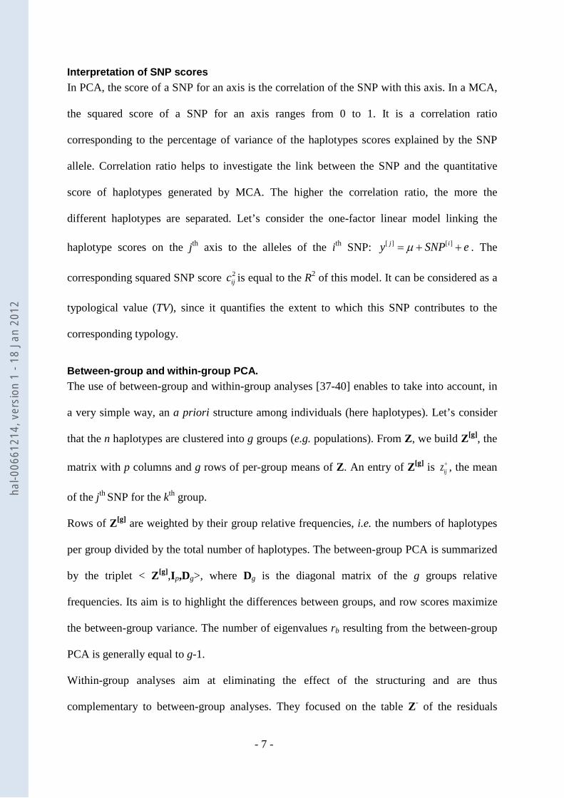
Interpretation of SNP scores In PCA, the score of a SNP for an axis is the correlation of the SNP with this axis. In a MCA,
the squared score of a SNP for an axis ranges from 0 to 1. It is a correlation ratio
corresponding to the percentage of variance of the haplotypes scores explained by the SNP
allele. Correlation ratio helps to investigate the link between the SNP and the quantitative
score of haplotypes generated by MCA. The higher the correlation ratio, the more the
different haplotypes are separated. Let’s consider the one-factor linear model linking the
haplotype scores on the jth axis to the alleles of the ith SNP: [ ] [ ]j iy SNP eµ= + + . The
corresponding squared SNP score 2ijc is equal to the R2 of this model. It can be considered as a
typological value (TV), since it quantifies the extent to which this SNP contributes to the
corresponding typology.
Between-group and within-group PCA. The use of between-group and within-group analyses [37-40] enables to take into account, in
a very simple way, an a priori structure among individuals (here haplotypes). Let’s consider
that the n haplotypes are clustered into g groups (e.g. populations). From Z, we build Z[g], the
matrix with p columns and g rows of per-group means of Z. An entry of Z[g] is ijz+ , the mean
of the jth SNP for the kth group.
Rows of Z[g] are weighted by their group relative frequencies, i.e. the numbers of haplotypes
per group divided by the total number of haplotypes. The between-group PCA is summarized
by the triplet < Z[g],Ip,Dg>, where Dg is the diagonal matrix of the g groups relative
frequencies. Its aim is to highlight the differences between groups, and row scores maximize
the between-group variance. The number of eigenvalues rb resulting from the between-group
PCA is generally equal to g-1.
Within-group analyses aim at eliminating the effect of the structuring and are thus
complementary to between-group analyses. They focused on the table Z- of the residuals
hal-0
0661
214,
ver
sion
1 -
18 J
an 2
012
- 8 -
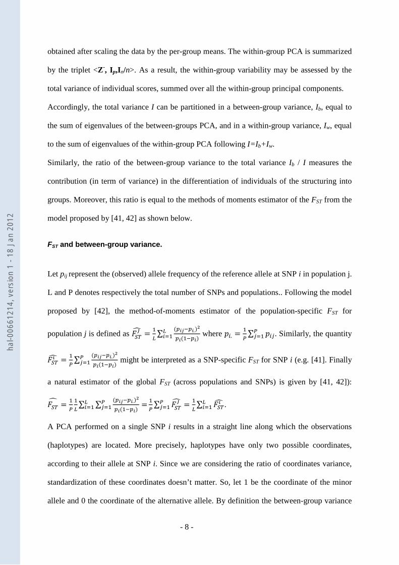
obtained after scaling the data by the per-group means. The within-group PCA is summarized
by the triplet <Z-, Ip,In/n>. As a result, the within-group variability may be assessed by the
total variance of individual scores, summed over all the within-group principal components.
Accordingly, the total variance I can be partitioned in a between-group variance, Ib, equal to
the sum of eigenvalues of the between-groups PCA, and in a within-group variance, Iw, equal
to the sum of eigenvalues of the within-group PCA following I=Ib+Iw.
Similarly, the ratio of the between-group variance to the total variance Ib / I measures the
contribution (in term of variance) in the differentiation of individuals of the structuring into
groups. Moreover, this ratio is equal to the methods of moments estimator of the FST from the
model proposed by [41, 42] as shown below.
FST and between-group variance.
Let pij represent the (observed) allele frequency of the reference allele at SNP i in population j.
L and P denotes respectively the total number of SNPs and populations.. Following the model
proposed by [42], the method-of-moments estimator of the population-specific FST for
population j is defined as 𝐹𝑆𝑇𝚥� = 1
𝐿∑ (𝑝𝑖𝑗−𝑝𝑖.)2
𝑝𝑖(1−𝑝𝑖)𝐿𝑖=1 where 𝑝𝑖. = 1
𝑃∑ 𝑝𝑖𝑗𝑃𝑗=1 . Similarly, the quantity
𝐹𝑆𝑇𝚤� = 1𝑃∑ (𝑝𝑖𝑗−𝑝𝑖.)2
𝑝𝑖(1−𝑝𝑖)𝑃𝑗=1 might be interpreted as a SNP-specific FST for SNP i (e.g. [41]. Finally
a natural estimator of the global FST (across populations and SNPs) is given by [41, 42]):
𝐹𝑆𝑇� = 1
𝑃1𝐿∑ ∑ (𝑝𝑖𝑗−𝑝𝑖.)2
𝑝𝑖(1−𝑝𝑖)𝑃𝑗=1 =𝐿
𝑖=11𝑃∑ 𝐹𝑆𝑇
𝚥�𝑃𝑗=1 = 1
𝐿∑ 𝐹𝑆𝑇𝚤�𝐿𝑖=1 .
A PCA performed on a single SNP i results in a straight line along which the observations
(haplotypes) are located. More precisely, haplotypes have only two possible coordinates,
according to their allele at SNP i. Since we are considering the ratio of coordinates variance,
standardization of these coordinates doesn’t matter. So, let 1 be the coordinate of the minor
allele and 0 the coordinate of the alternative allele. By definition the between-group variance
hal-0
0661
214,
ver
sion
1 -
18 J
an 2
012
- 9 -
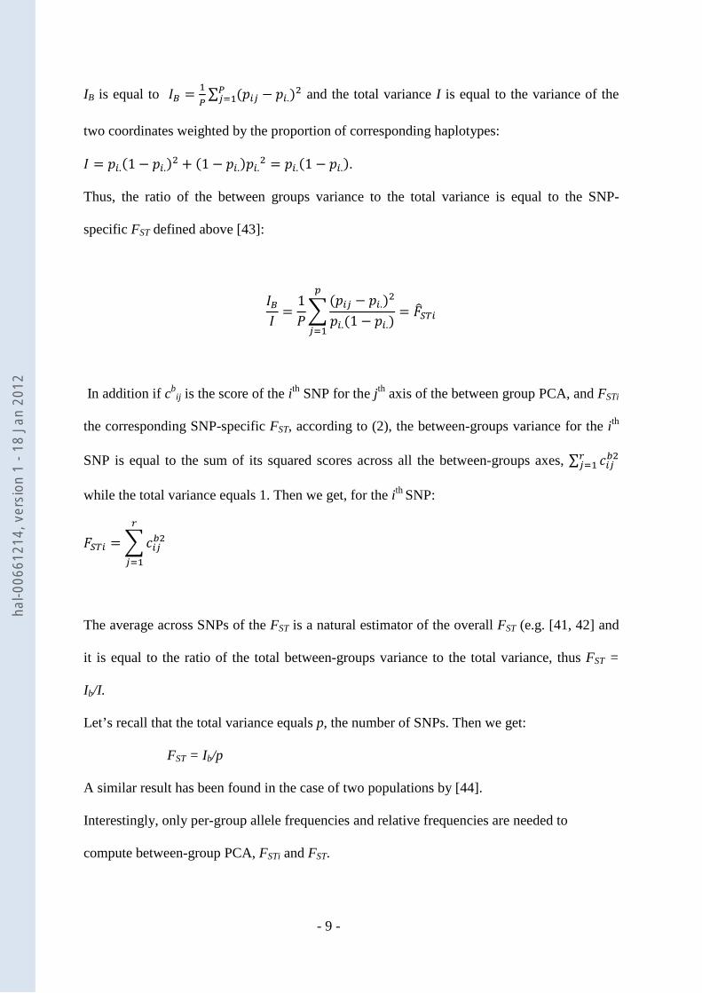
IB is equal to 𝐼𝐵 = 1𝑃∑ (𝑝𝑖𝑗 − 𝑝𝑖.)2𝑃𝑗=1 and the total variance I is equal to the variance of the
two coordinates weighted by the proportion of corresponding haplotypes:
𝐼 = 𝑝𝑖.(1 − 𝑝𝑖.)2 + (1 − 𝑝𝑖.)𝑝𝑖.2 = 𝑝𝑖.(1 − 𝑝𝑖.).
Thus, the ratio of the between groups variance to the total variance is equal to the SNP-
specific FST defined above [43]:
𝐼𝐵𝐼
=1𝑃�
(𝑝𝑖𝑗 − 𝑝𝑖.)2
𝑝𝑖.(1 − 𝑝𝑖.)
𝑝
𝑗=1
= 𝐹�𝑆𝑇𝑖
In addition if cbij is the score of the ith SNP for the jth axis of the between group PCA, and FSTi
the corresponding SNP-specific FST, according to (2), the between-groups variance for the ith
SNP is equal to the sum of its squared scores across all the between-groups axes, ∑ 𝑐𝑖𝑗𝑏2𝑟𝑗=1
while the total variance equals 1. Then we get, for the ith SNP:
𝐹𝑆𝑇𝑖 = �𝑐𝑖𝑗𝑏2𝑟
𝑗=1
The average across SNPs of the FST is a natural estimator of the overall FST (e.g. [41, 42] and
it is equal to the ratio of the total between-groups variance to the total variance, thus FST =
Ib/I.
Let’s recall that the total variance equals p, the number of SNPs. Then we get:
FST = Ib/p
A similar result has been found in the case of two populations by [44].
Interestingly, only per-group allele frequencies and relative frequencies are needed to
compute between-group PCA, FSTi and FST.
hal-0
0661
214,
ver
sion
1 -
18 J
an 2
012
- 10 -
Applications to a human dataset. To illustrate these different interpretations of PCA results, we analyzed human chromosome 2
(HSA2) 116,430 SNPs haplotypes for three populations: CEU (Utah residents with ancestry
from northern and western Europe), YRI (Yoruba in Ibadan, Nigeria) and CHB+JPT (Han
Chinese in Beijing, China and Japanese in Tokyo, Japan). The total variance equals 116,053,
i.e. the number of polymorphic SNPs. The first and second between PCA eigenvalues are
equal to 8,004 (7 % of the total variance) and 3,881 (3% of the total variance), respectively
while the within-population PCA eigenvalues are varying from 31 to 315. The resulting
global FST equals 0.1024, computed as described above, and is close to those previously
reported using the Phase 1 HapMap data [45]
The within population variability were equal to 137,163, 104,219 and 82,891 for YRI, CEU
and JPT+CHB, respectively. These results are also consistent with [7] which reported that
heterozygosity is the highest in subsaharian Africa, intermediate in Europa and the smallest in
East Asia.
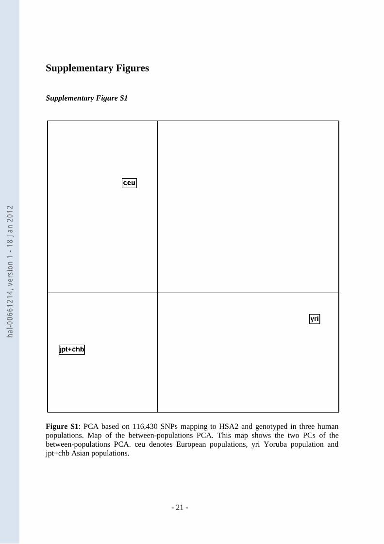
The factorial map of the between-populations analysis is given in Figure S1. Since there are
three populations, two axes are sufficient to summarize the total variation between the three
populations. The first axis isolates YRI population from CEU and CHB+JPT, while the
second axis isolates CEU. Corresponding spatial autocorrelations of SNPs correlation ratio
are equal to 0.27 and 0.31, respectively. Plots of SNP TVs for axes 1 and 2 and their SNP-
specific FST (corresponding to the sum of TVs of the two axes) are given in Supplementary
Figures 2. However, to better assess regions with large amount of SNPs displaying high TVs,
we adopted an empirical smoothing approach inspired from [45] which consisted in averaging
TVs (and SNP-specific FST) over 3-Mb sliding windows. As a matter of expedience, for each
axis (and for FST), two thresholds were considered to identify outlying smoothed score,
respectively 2.32 and 3.09 (empirical) standard deviations from the (empirical) average. If the
score distributions were Gaussian under the null hypothesis of neutrality, these thresholds
hal-0
0661
214,
ver
sion
1 -
18 J
an 2
012
- 11 -
would correspond to standard 0.01 and 0.001 p-values. However, they might be less
conservative since the observed distribution had a fatter tail than a Gaussian distribution as a
probable result from the biased choice of the chromosome in which several footprints of
selection have already been detected (see below). From a genome-wide perspective (beyond
the scope of this illustrative example), this might be less of concern.
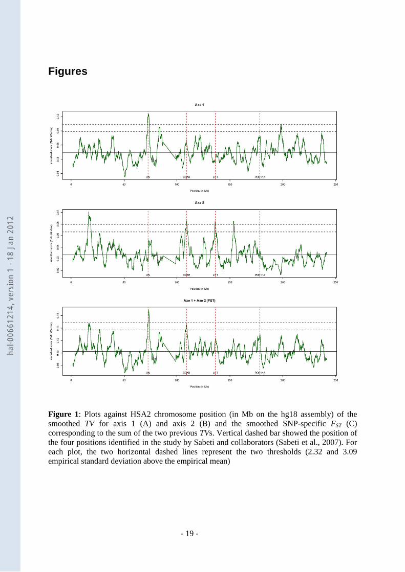
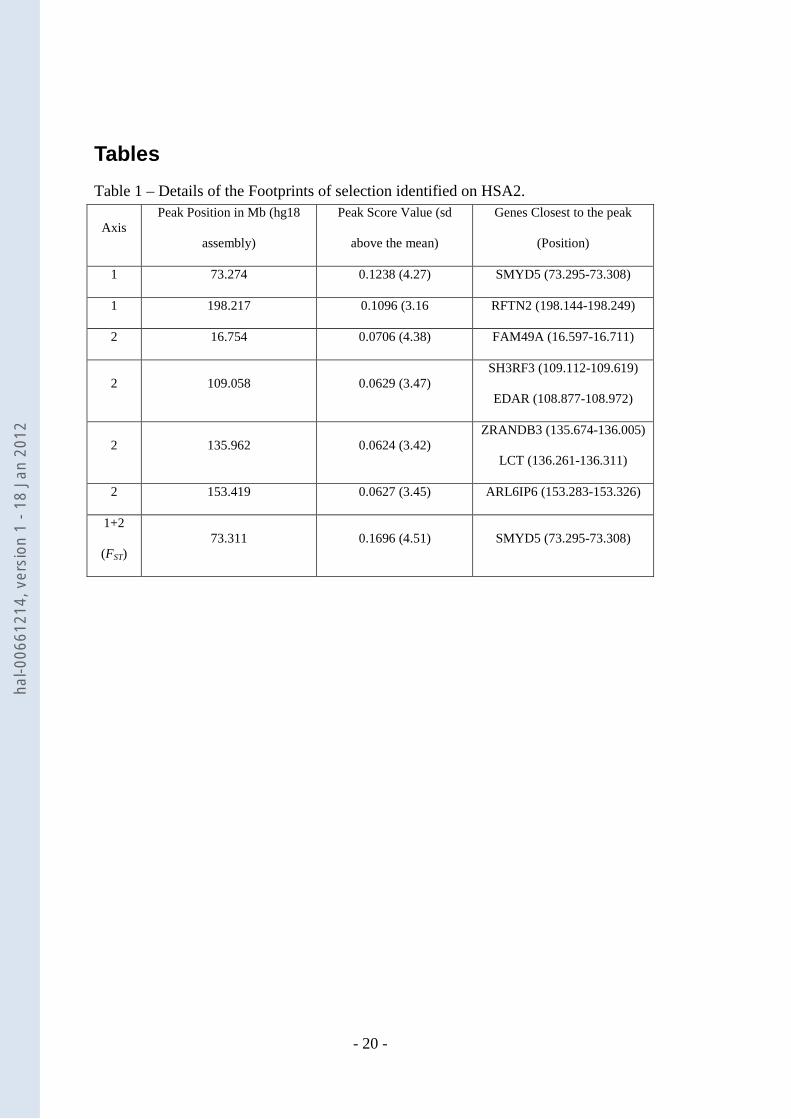
The three different smoothed scores are plotted in Figure 1 and significant peak positions are
detailed in Table 1. For the first axis which separated YRI from the two others populations,
two significant peaks (with a smoothed score greater than 3.09 standard deviations above the
mean) were observed at positions 73.3 Mb and 198.2 Mb. For the second axis which
separated CEU from the two others populations, four significant peaks were observed at
positions 16.754 Mb, 109.058 Mb, 135.962 Mb and 153.419 Mb. Finally, when considering
the smoothed score based on the sum of TV for the two axes (i.e. FST), only one (at position
73.3 Mb) of the previous peaks was found as being still significant. Overall, these results are
consistent with previous published studies. For instance, Sabeti and collaborators [46]
reported four regions on HSA2 as subjected to selection (around positions 72.5 Mb, 108.6
Mb, 136.0 Mb and 177.7 Mb when converted to hg18 genome assembly positions) based on
the XP-EHH test in JPT+CHB, JPT+CHB, CEU and both CEU and JPT+CHB populations
respectively. Hence three of these positions were close (less then 500 kb) or confounded with
peak identified on second axis although the first two signals were found significant in
JPT+CHB population in this latter study. Interestingly, the third position (around 136.0 Mb)
within the ZRANDB3 gene (Table 1) is close to the LCT gene (less than 300 kb) which has
been extensively reported as a putative target for natural selection and within which an allele
have been found at high frequency within Europe, absent in the Yoruba population and almost
absent in East Asia [47]. Similarly, the second peak observed on Axis 2 is close (less than 20
kb) to EDAR which was previously identified as the putative target of a strong selective
hal-0
0661
214,
ver
sion
1 -
18 J
an 2
012
- 12 -
sweep in East Asians [48]. Finally, three additional peaks were identified in our study and
have not been reported elsewhere. They are located close or within RFTN2, FAM49A and
ARL6IP6 genes.
Discussion PCA is primarily an exploratory technique and it is now almost exclusively based upon
individual-level rather than population-level analyses. However, prior knowledge about the
structuring of the populations under study can be explicitly taken into account by partitioning
the ordinary PCA in sub-analyses. Interestingly, a between-population analysis delivers
standard estimates of FST (either population-specific or SNP specific). This is, for instance, of
particular interest in the case of highly structured populations such as cattle [16]. In our
application, confirming previous results, the first PC isolates the African population from the
two others, while the second PC contrasts Europeans with Africans and Asians (Figure S1).
Within-group PCA enabled to assess within-population diversity and to compare the different
populations according to this criterion. Our results were in agreement with previous ones that
showed more genetic diversity in African populations.
Because of PCA flexibility, such an approach might also be extended to several other factors
and a multi-factorial or nested stratification (e.g populations nested in continents, or
population crossed with some disease sensibility) may be accounted for by a modification of
PCA involving the so-called “instrumental variables” [32, 40]. Such analyses should enable to
rule out known genetic structuring by adjusting for these factors or alternatively to quantify
the TV of SNPs according to each of them.
hal-0
0661
214,
ver
sion
1 -
18 J
an 2
012
- 13 -
For instance, in this paper, we investigated some features of a normed PCA applied to SNP
haplotypes for quantifying the typological value of a SNP regarding a principal component.
Because TV is a correlation ratio, quantifying the reduction of variance of haplotypes scores
due to the knowledge/ascertainment of the SNP allelic form, a small value indicates that the
marker does not contribute to the building of the component. Conversely, a value close to 1
indicates that the typology is completely built by the SNP and might thus be related to
putative signal of selection [29]. Moreover, TVs are also FST, that has been advocated to
identify regions of the genome that have been the target of selection [31, 45, 49, 50]. More
specifically, our approach might be regarded as equivalent to recently proposed model-based
approaches aiming at identifying population-specific effect of SNP contribution to overall
differentiation while taking into account hierarchical structure among populations under study
[51] although PCA remains by far more computational efficient.
In addition, TVs may help to analyze how the position of markers along a chromosome
impacts their contributions to the genetic diversity. Therefore, plots of the TVs with respect to
the position of the underlying SNP along the chromosomes enable to easily spot candidate
regions for footprints of selection which are expected to display several SNPs with high
typological values. This was exemplified by our application on HSA2 haplotypes where
several footprints of selection had already been reported [46, 48]. Note, that in order to take
into account spatial dependency among SNPs along the haplotypes TVs we adopted an
empirical smoothing approach [45] which consisted in averaging scores over 3-Mb sliding
windows. Due to the properties of the scores, model-based strategies might be more adapted
and more rigorous to identify such outlier regions and to propose better significance
thresholds. To that regard, analyses of SNP scores with autoregressive models represent for
instance promising alternatives as recently illustrated under a Bayesian framework by Guo
and collaborators [52] who investigated Conditionally Autoregressive models (CAR) models
hal-0
0661
214,
ver
sion
1 -
18 J
an 2
012
- 14 -
to identify local effect on SNP differentiation. Finally, relating TV to their underlying axe
helps to better refine the putative origin of the signal and gives a more precise picture
compared to the one obtained when considering SNP-specific FST across populations (see
Figure 1).
Conclusions Since Cavalli-Sforza advocated using PCA to decipher population structuring of genetic
diversity [2], this approach and related factorial methods have been proved useful to address
other issues such as correcting for stratification in genome-wide studies [53], assessing the TV
of markers [4, 27], addressing the spatial structuring of genetic diversity [16, 54, 55],
identifying small subsets of informative SNPs [25, 26], simultaneous accounting for genetic
and morphologic data [56], and discriminating among populations [29].
The main advantages of PCA are its versatility and its computational efficiency allowing to
deal with large data sets currently produced [3].We hope that the enhanced interpretation of
the PCA results when dealing with biallelic SNPs will give another argument for using it.
Material and Methods Haplotype Data Human chromosome 2 haplotype data were downloaded from the HAPMAP project website
(http://hapmap.ncbi.nlm.nih.gov/downloads/phasing/2009-02_phaseIII/) wheremore details
can be found. Respectively, 231 CEU, 234 YRI and 339 JPT+CHB haplotypes were
considered in the analysis. Each haplotype consisted of 116,430 SNPs.
hal-0
0661
214,
ver
sion
1 -
18 J
an 2
012
- 15 -
Analyses Within and between populations PCA were performed with the R software [57] and the R
package ade4 (more particularly dudi.pca, between and within functions) [58].
Authors' contributions DL conceived of the study, analyzed the data and wrote the manuscript.
MG participated to data analysis and wrote the manuscript.
Both authors read and approved the final manuscript.
Acknowledgements Research was supported in part by the French ANR (contract “BLANC” “EMILE” NT09-
611697).
References
1. Pritchard JK, Stephens M, Donnelly P: Inference of population structure using multilocus genotype data. Genetics 2000, 155(2):945-959.
2. Cavalli-Sforza LL: Population structure and human evolution. Proceedings of the Royal Society Series B-Biological Sciences 1966, 164(995):362-379.
3. Jombart T, Pontier D, Dufour AB: Genetic markers in the playground of multivariate analysis. Heredity 2009, 102(4):330-341.
4. Moazami-Goudarzi K, Laloe D: Is a multivariate consensus representation of genetic relationships among populations always meaningful? Genetics 2002, 162(1):473-484.
5. Patterson N, Price AL, Reich D: Population structure and eigenanalysis. Plos Genetics 2006, 2(12):2074-2093.
6. Pearson K: On lines and planes of closest fit to systems of points in space. Philosophical Magazine 1901, 2:559-572.
7. Li JZ, Absher DM, Tang H, Southwick AM, Casto AM, Ramachandran S, Cann HM, Barsh GS, Feldman M, Cavalli-Sforza LL et al: Worldwide human relationships inferred from genome-wide patterns of variation. Science 2008, 319(5866):1100-1104.
8. Tang H, Coram M, Wang P, Zhu X, Risch N: Reconstructing genetic ancestry blocks in admixed individuals. American Journal of Human Genetics 2006, 79(1):1-12.
9. Alexander DH, Novembre J, Lange K: Fast model-based estimation of ancestry in unrelated individuals. Genome Research 2009, 19(9):1655-1664.
hal-0
0661
214,
ver
sion
1 -
18 J
an 2
012
- 16 -
10. Auton A, Bryc K, Boyko AR, Lohmueller KE, Novembre J, Reynolds A, Indap A, Wright MH, Degenhardt JD, Gutenkunst RN et al: Global distribution of genomic diversity underscores rich complex history of continental human populations. Genome Research 2009, 19(5):795-803.
11. Lao O, Lu TT, Nothnagel M, Junge O, Freitag-Wolf S, Caliebe A, Balascakova M, Bertranpetit J, Bindoff LA, Comas D et al: Correlation between Genetic and Geographic Structure in Europe. Current Biology 2008, 18(16):1241-1248.
12. Nelis M, Esko T, Mägi R, Zimprich F, Zimprich A, Toncheva D, Karachanak S, Piskáčková T, Balaščák I, Peltonen L et al: Genetic Structure of Europeans: A View from the North–East. PLoS ONE 2009, 4(5):e5472.
13. Heath SC, Gut IG, Brennan P, McKay JD, Bencko V, Fabianova E, Foretova L, Georges M, Janout V, Kabesch M et al: Investigation of the fine structure of European populations with applications to disease association studies.
14. The Bovine HapMap C, Gibbs RA, Taylor JF, Van Tassell CP, Barendse W, Eversole KA, Gill CA, Green RD, Hamernik DL, Kappes SM et al: Genome-Wide Survey of SNP Variation Uncovers the Genetic Structure of Cattle Breeds. Science 2009, 324(5926):528-532
15. Gautier M, Flori L, Riebler A, Jaffrezic F, Laloe D, Gut I, Moazami-Goudarzi K, Foulley JL: A whole genome Bayesian scan for adaptive genetic divergence in West African cattle. BMC Genomics 2009, 10:550.
16. Gautier M, Laloe D, Moazami-Goudarzi K: Insights into the genetic history of French cattle from dense SNP data on 47 worldwide breeds. PLoS One 2010, 5(9).
17. Horne BD, Camp NJ: Principal component analysis for selection of optimal SNP-sets that capture intragenic genetic variation. Genetic Epidemiology 2004, 26(1):11-21.
18. Zhang FY, Wagener D: An approach to incorporate linkage disequilibrium structure into genomic association analysis. Journal of Genetics and Genomics 2008, 35(6):381-385.
19. Hill WG, Robertson A: Linkage disequilibrium in finite populations. Theor Appl Genet 1968, 38:226 - 231.
20. Dray S, Dufour AB: The ade4 package: Implementing the duality diagram for ecologists. Journal of Statistical Software 2007, 22(4):1-20.
21. Cailliez F, Pages JP: Introduction à l'analyse des données. Paris: SMASH; 1976. 22. Guyon I, Elisseeff A: An introduction to variable and feature selection. Journal of
Machine Learning Research 2003, 3:1157-1182. 23. Zou H, Hastie T: Regularization and variable selection via the elastic net. Journal
of the Royal Statistical Society Series B-Statistical Methodology 2005, 67:301-320. 24. Zou H, Hastie T, Tibshirani R: Sparse principal component analysis. Journal of
Computational and Graphical Statistics 2006, 15(2):265-286. 25. Paschou P, Ziv E, Burchard EG, Choudhry S, Rodriguez-Cintron W, Mahoney MW,
Drineas P: PCA-correlated SNPs for structure identification in worldwide human populations. Plos Genetics 2007, 3:1672-1686.
26. Paschou P, Lewis J, Javed A, Drineas P: Ancestry informative markers for fine-scale individual assignment to worldwide populations. Journal of Medical Genetics 2010, 47(12):835-847.
27. Laloe D, Jombart T, Dufour AB, Moazami-Goudarzi K: Consensus genetic structuring and typological value of markers using multiple co-inertia analysis. Genetics Selection Evolution 2007, 39(5):545-567.
28. Park S, Ku YK, Seo MJ, Kim DY, Yeon JE, Lee KM, Jeong SC, Yoon WK, Harn CH, Kim HM: Principal component analysis and discriminant analysis (PCA-DA) for
hal-0
0661
214,
ver
sion
1 -
18 J
an 2
012
- 17 -
discriminating profiles of terminal restriction fragment length polymorphism (T-RFLP) in soil bacterial communities. Soil Biology & Biochemistry 2006, 38(8):2344-2349.
29. Jombart T, Devillard S, Balloux F: Discriminant analysis of principal components: a new method for the analysis of genetically structured populations. BMC Genet 2010, 11:94.
30. Tenenhaus M, Young FW: An analysis and synthesis of Multiple Correspondence Analysis, Optimal Scaling, Dual Scaling, Homogeneity Analysis and other methods for quantifying categorical multivariate data. Psychometrika 1985, 50(1):91-119.
31. Holsinger KE, Weir BS: FUNDAMENTAL CONCEPTS IN GENETICS Genetics in geographically structured populations: defining, estimating and interpreting F-ST. Nature Reviews Genetics 2009, 10(9):639-650.
32. Jolliffe IT: Principal Component Analysis, 2 edn. New York: Springer; 2002. 33. Escofier B: Une représentation des variables dans l'analyse des correspondance
multiples. Revue de Statistique Appliquée 1979, 27(4):37-47. 34. Fisher RA: The precision of discriminant functions. Annals of Eugenics 1940,
10:422-429. 35. Benzecri JP: L'analyse des données. I. L'analyse des correspondances. Paris:
Dunod; 1973. 36. Greenacre MJ: Theory and Applications of Correspondence Analysis. London:
Academic Press; 1984. 37. Rao CR: The use and interpretation of principal components analysis in applied
research. Sankhya A 1964, 26:329-359. 38. Doledec S, Chessel D: Seasonal successions and spatial variables in fresh-water
environments. 1.Description of a complete 2-way layout by projection of variables. Acta Oecologica-Oecologia Generalis 1987, 8(3):403-426.
39. Culhane AC, Perriere G, Considine EC, Cotter TG, Higgins DG: Between-group analysis of microarray data. Bioinformatics 2002, 18(12):1600-1608.
40. Baty F, Facompre M, Wiegand J, Schwager J, Brutsche MH: Analysis with respect to instrumental variables for the exploration of microarray data structures. Bmc Bioinformatics 2006, 7.
41. Flori L, Fritz S, Jaffrezic F, Boussaha M, Gut I, Heath S, Foulley JL, Gautier M: The genome response to artificial selection: a case study in dairy cattle. PLoS One 2009, 4(8):e6595.
42. Nicholson G, Smith AV, Jonsson F, Gustafsson O, Stefansson K, Donnelly P: Assessing population differentiation and isolation from single-nucleotide polymorphism data. Journal of the Royal Statistical Society Series B-Statistical Methodology 2002, 64:695-715.
43. Chessel D, Laloë D: Les tableaux de fréquences alléliques. [http://pbil.univ-lyon1.fr/R/pdf/thema2D.pdf]
44. McVean G: A Genealogical Interpretation of Principal Components Analysis. Plos Genetics 2009, 5(10).
45. Weir BS, Cardon LR, Anderson AD, Nielsen DM, Hill WG: Measures of human population structure show heterogeneity among genomic regions. Genome Research 2005, 15(11):1468-1476.
46. Sabeti PC, Varilly P, Fry B, Lohmueller J, Hostetter E, Cotsapas C, Xie XH, Byrne EH, McCarroll SA, Gaudet R et al: Genome-wide detection and characterization of positive selection in human populations. Nature 2007, 449(7164):913-U912.
hal-0
0661
214,
ver
sion
1 -
18 J
an 2
012
- 18 -
47. Bersaglieri T, Sabeti PC, Patterson N, Vanderploeg T, Schaffner SF, Drake JA, Rhodes M, Reich DE, Hirschhorn JN: Genetic signatures of strong recent positive selection at the lactase gene. American Journal of Human Genetics 2004, 74(6):1111-1120.
48. Xue YL, Zhang XL, Huang N, Daly A, Gillson CJ, MacArthur DG, Yngvadottir B, Nica AC, Woodwark C, Chen Y et al: Population Differentiation as an Indicator of Recent Positive Selection in Humans: An Empirical Evaluation. Genetics 2009, 183(3):1065-1077.
49. Akey JM, Zhang G, Zhang K, Jin L, Shriver MD: Interrogating a high-density SNP map for signatures of natural selection. Genome Research 2002, 12(12):1805-1814.
50. Beaumont MA, Balding DJ: Identifying adaptive genetic divergence among populations from genome scans. Molecular Ecology 2004, 13(4):969-980.
51. Coop G, Witonsky D, Di Rienzo A, Pritchard JK: Using Environmental Correlations to Identify Loci Underlying Local Adaptation. Genetics 2010, 185(4):1411-1423.
52. Guo F, Dey DK, Holsinger KE: A Bayesian Hierarchical Model for Analysis of Single-Nucleotide Polymorphisms Diversity in Multilocus, Multipopulation Samples. Journal of the American Statistical Association 2009, 104(485):142-154.
53. Price AL, Patterson NJ, Plenge RM, Weinblatt ME, Shadick NA, Reich D: Principal components analysis corrects for stratification in genome-wide association studies. Nat Genet 2006, 38(8):904-909.
54. Laloë D, Moazami-Goudarzi K, Lenstra JA, Marsan PA, Azor P, Baumung R, Bradley DG, Bruford MW, Cañón J, Dolf G et al: Spatial Trends of Genetic Variation of Domestic Ruminants in Europe. Diversity 2010, 2(6):932-945.
55. Jombart T, Devillard S, Dufour AB, Pontier D: Revealing cryptic spatial patterns in genetic variability by a new multivariate method. Heredity 2008, 101(1):92-103.
56. Berthouly C, Rognon X, Van TN, Berthouly A, Hoang HT, Bed'Hom B, Laloe D, Chi CV, Verrier E, Maillard JC: Genetic and morphometric characterization of a local Vietnamese Swamp Buffalo population. Journal of Animal Breeding and Genetics 2010, 127(1):74-84.
57. R Development Core Team: R: A language and environment for statistical computing. 2009 [http://www.r-project.org]
58. Chessel D, Dufour AB, Thioulouse J: The ade4 package. I. One-table methods. R News 2004, 4:5-10.
hal-0
0661
214,
ver
sion
1 -
18 J
an 2
012
- 19 -
Figures
Figure 1: Plots against HSA2 chromosome position (in Mb on the hg18 assembly) of the smoothed TV for axis 1 (A) and axis 2 (B) and the smoothed SNP-specific FST (C) corresponding to the sum of the two previous TVs. Vertical dashed bar showed the position of the four positions identified in the study by Sabeti and collaborators (Sabeti et al., 2007). For each plot, the two horizontal dashed lines represent the two thresholds (2.32 and 3.09 empirical standard deviation above the empirical mean)
hal-0
0661
214,
ver
sion
1 -
18 J
an 2
012
- 20 -
Tables Table 1 – Details of the Footprints of selection identified on HSA2.
Axis Peak Position in Mb (hg18
assembly)
Peak Score Value (sd
above the mean)
Genes Closest to the peak
(Position)
1 73.274 0.1238 (4.27) SMYD5 (73.295-73.308)
1 198.217 0.1096 (3.16 RFTN2 (198.144-198.249)
2 16.754 0.0706 (4.38) FAM49A (16.597-16.711)
2 109.058 0.0629 (3.47) SH3RF3 (109.112-109.619)
EDAR (108.877-108.972)
2 135.962 0.0624 (3.42) ZRANDB3 (135.674-136.005)
LCT (136.261-136.311)
2 153.419 0.0627 (3.45) ARL6IP6 (153.283-153.326)
1+2
(FST) 73.311 0.1696 (4.51) SMYD5 (73.295-73.308)
hal-0
0661
214,
ver
sion
1 -
18 J
an 2
012
- 21 -
Supplementary Figures
Supplementary Figure S1
Figure S1: PCA based on 116,430 SNPs mapping to HSA2 and genotyped in three human populations. Map of the between-populations PCA. This map shows the two PCs of the between-populations PCA. ceu denotes European populations, yri Yoruba population and jpt+chb Asian populations.
hal-0
0661
214,
ver
sion
1 -
18 J
an 2
012
- 22 -
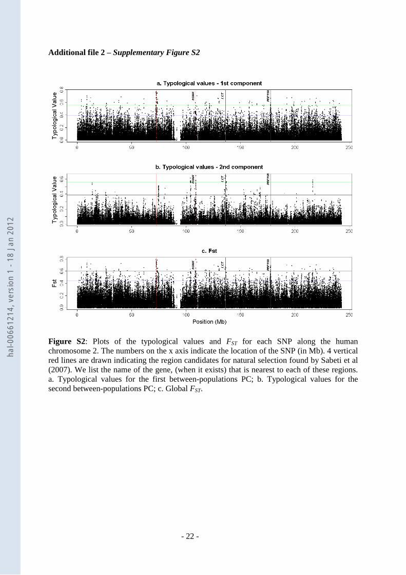
Additional file 2 – Supplementary Figure S2
Figure S2: Plots of the typological values and FST for each SNP along the human chromosome 2. The numbers on the x axis indicate the location of the SNP (in Mb). 4 vertical red lines are drawn indicating the region candidates for natural selection found by Sabeti et al (2007). We list the name of the gene, (when it exists) that is nearest to each of these regions. a. Typological values for the first between-populations PC; b. Typological values for the second between-populations PC; c. Global FST.
hal-0
0661
214,
ver
sion
1 -
18 J
an 2
012
- 23 -
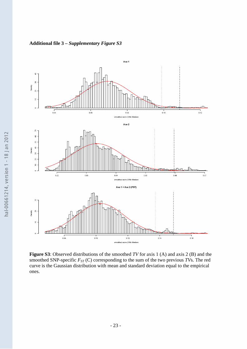
Additional file 3 – Supplementary Figure S3
Figure S3: Observed distributions of the smoothed TV for axis 1 (A) and axis 2 (B) and the smoothed SNP-specific FST (C) corresponding to the sum of the two previous TVs. The red curve is the Gaussian distribution with mean and standard deviation equal to the empirical ones.
hal-0
0661
214,
ver
sion
1 -
18 J
an 2
012