On the Geometric Dilation of Closed Curves, Graphs, and ...the+geometric... · arXiv:math.MG/0407135 v2 25 Aug 2005 On the Geometric Dilation of Closed Curves, Graphs, and Point Sets∗

arX

iv:m

ath.

MG

/040

7135

v2

25

Aug

200

5

On the Geometric Dilation of Closed Curves, Graphs,

and Point Sets∗

Adrian Dumitrescu† Annette Ebbers-Baumann‡ Ansgar Grune‡¶

Rolf Klein‡‖ Gunter Rote§

August 25, 2005

Abstract

Let G be an embedded planar graph whose edges are curves. The detour betweentwo points p and q (on edges or vertices) of G is the ratio between the length of a shortestpath connecting p and q in G and their Euclidean distance |pq|. The maximum detourover all pairs of points is called the geometric dilation δ(G).

Ebbers-Baumann, Grune and Klein have shown that every finite point set is con-tained in a planar graph whose geometric dilation is at most 1.678, and some point setsrequire graphs with dilation δ ≥ π/2 ≈ 1.57. They conjectured that the lower boundis not tight.

We use new ideas like the halving pair transformation, a disk packing result and ar-guments from convex geometry, to prove this conjecture. The lower bound is improvedto (1 + 10−11)π/2. The proof relies on halving pairs, pairs of points dividing a givenclosed curve C in two parts of equal length, and their minimum and maximum dis-tances h and H . Additionally, we analyze curves of constant halving distance (h = H),examine the relation of h to other geometric quantities and prove some new dilationbounds.

Key words: computational geometry, convex geometry, convex curves, dilation, distor-tion, detour, lower bound, halving chord, halving pair, Zindler curves

∗Some results of this article were presented at the 21st European Workshop on Computational Geometry(EWCG ’05)[7], others at the 9th Workshop on Algorithms and Data Structures (WADS ’05)[6].

†Computer Science, University of Wisconsin–Milwaukee, 3200 N. Cramer Street, Milwaukee, WI 53211,USA; [email protected]

‡Institut fur Informatik I, Universitat Bonn, Romerstraße 164, D - 53117 Bonn, Germany;ebbers, gruene, [email protected]

§Freie Universitat Berlin, Institut fur Informatik, Takustraße 9, D-14195 Berlin, Germany;[email protected]

¶Ansgar Grune was partially supported by a DAAD PhD-grant.‖Rolf Klein was partially supported by DFG-grant KL 655/14-1.

1

Preprint submitted to Elsevier Science 25th August 2005

1 Introduction

Consider a planar graph G embedded in R2, whose edges are curves1 that do not intersect.Such graphs arise naturally in the study of transportation networks, like waterways, railroadsor streets. For two points, p and q (on edges or vertices) of G, the detour between p and qin G is defined as

δG(p, q) =dG(p, q)

|pq|where dG(p, q) is the shortest path length in G between p and q, and |pq| denotes theEuclidean distance, see Figure 1a for an illustration. Good transportation networks should

p

q

|pq|

dG(p, q)

G

(a)

√

3

1

2

1

2

1

1

3

√

3p

q

(b)

Figure 1: (a) The shortest path (dashed) between p and q in the graph G and the directdistance |pq|. (b) Three points (drawn as empty circles) embedded in a hexagonal grid withgeometric dilation

√3 ≈ 1.732.

have small detour values. In a railroad system, access is only possible at stations, the verticesof the graph. Hence, to measure the quality of such networks, we can take the maximumdetour over all pairs of vertices. This results in the well-known concept of graph-theoreticdilation studied extensively in the literature on spanners, see [11] for a survey.

However, if we consider a system of urban streets, houses are usually spread everywherealong the streets. Hence, we have to take into account not only the vertices of the graphbut all the points on its edges. The resulting supremum value is the geometric dilation

δ(G) := supp,q∈G

δG(p, q) = supp,q∈G

dG(p, q)

|pq|

on which we concentrate in this article. Several papers [10, 17, 2] have shown how toefficiently compute the geometric dilation of polygonal curves. Besides this the geometricdilation was studied in differential geometry and knot theory under the notion of distortion,see e.g. [13, 16].

1For simplicity we assume here that the curves are piecewise continuously differentiable, but most of theproofs can be extended to arbitrary rectifiable curves.

2


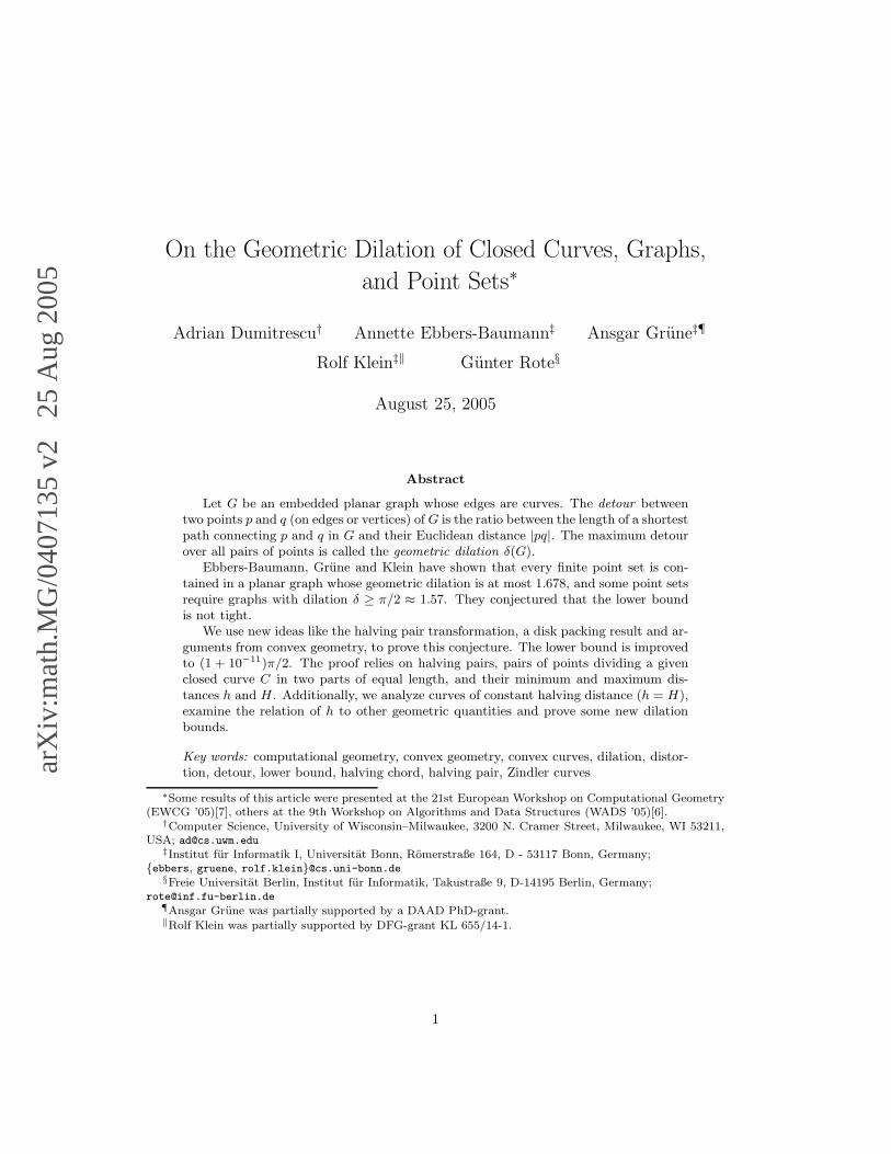
Figure 2: A section of the grid from [8] which has small dilation, less than 1.678.

Ebbers-Baumann et al. [8] recently considered the problem of constructing a graph of lowestpossible geometric dilation containing a given finite point set on its edges. Even for threegiven points this is not a trivial task. For some examples, clearly a Steiner-tree with threestraight line segments is optimal. In other cases a path consisting of straight and curvedpieces is better, but it is not easy to prove its optimality.

Therefore, Ebbers-Baumann et al. concentrated on examining the dilation necessary to em-bed any finite point set, i.e. the value

∆ := supP⊂R2, P finite

infG⊃P, G finite

δ(G) .

The infimum is taken over all embedded planar graphs G with a finite number of vertices,where the edges may be curves like discussed above. For example, a scaled hexagonal gridcan clearly be used to embed any finite subset of Q ×

√3Q like the example in Figure 1b.

The geometric dilation√

3 ≈ 1.732 of this grid is attained between two midpoints of oppositeedges of a hexagon.

Ebbers-Baumann et al. introduced the improved grid shown in Figure 2 and proved that itsdilation is less than 1.678. They showed that a slightly perturbed version of the grid can beused to embed any finite point set. Thereby they proved ∆ < 1.678.

They also derived that ∆ ≥ π/2, by showing that a graph G has to contain a cycle to embeda certain point set P5 with low dilation, and by using that the dilation of every closedcurve2 C is bounded by δ(C) ≥ π/2.

They conjectured that this lower bound is not tight. It is known that circles are the onlycycles of dilation π/2, see [9, Corollary 23], [1, Corollary 3.3], [16], [13]. And intuitionsuggests that one cannot embed complicated point sets with dilation π/2 because every face

2In this paper we use the notions “cycle” and “closed curve” synonymously.

3


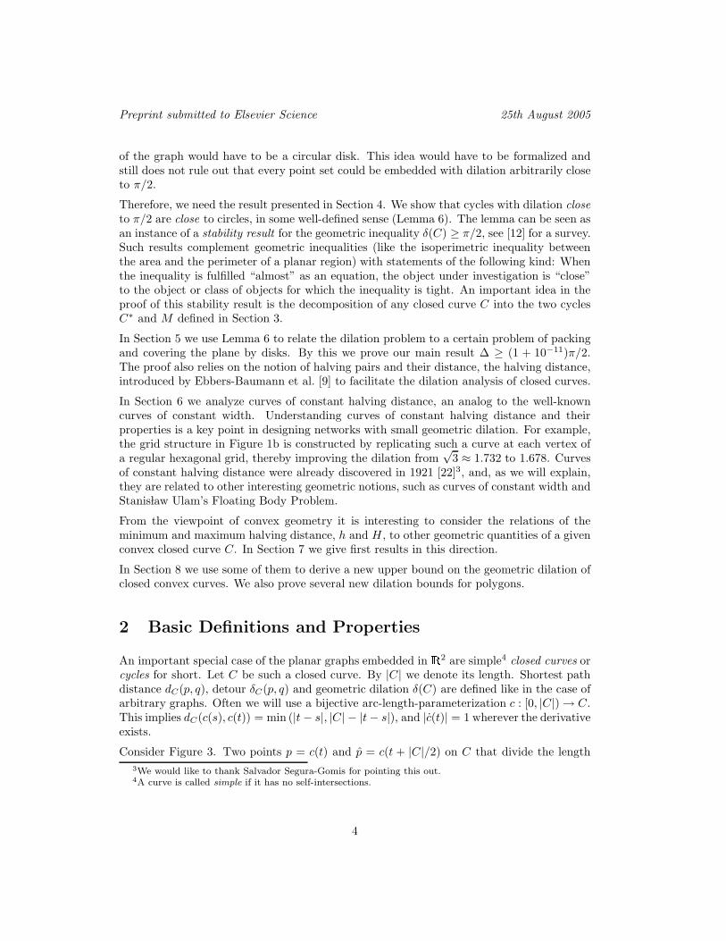
of the graph would have to be a circular disk. This idea would have to be formalized andstill does not rule out that every point set could be embedded with dilation arbitrarily closeto π/2.

Therefore, we need the result presented in Section 4. We show that cycles with dilation closeto π/2 are close to circles, in some well-defined sense (Lemma 6). The lemma can be seen asan instance of a stability result for the geometric inequality δ(C) ≥ π/2, see [12] for a survey.Such results complement geometric inequalities (like the isoperimetric inequality betweenthe area and the perimeter of a planar region) with statements of the following kind: Whenthe inequality is fulfilled “almost” as an equation, the object under investigation is “close”to the object or class of objects for which the inequality is tight. An important idea in theproof of this stability result is the decomposition of any closed curve C into the two cyclesC∗ and M defined in Section 3.

In Section 5 we use Lemma 6 to relate the dilation problem to a certain problem of packingand covering the plane by disks. By this we prove our main result ∆ ≥ (1 + 10−11)π/2.The proof also relies on the notion of halving pairs and their distance, the halving distance,introduced by Ebbers-Baumann et al. [9] to facilitate the dilation analysis of closed curves.

In Section 6 we analyze curves of constant halving distance, an analog to the well-knowncurves of constant width. Understanding curves of constant halving distance and theirproperties is a key point in designing networks with small geometric dilation. For example,the grid structure in Figure 1b is constructed by replicating such a curve at each vertex ofa regular hexagonal grid, thereby improving the dilation from

√3 ≈ 1.732 to 1.678. Curves

of constant halving distance were already discovered in 1921 [22]3, and, as we will explain,they are related to other interesting geometric notions, such as curves of constant width andStanis law Ulam’s Floating Body Problem.

From the viewpoint of convex geometry it is interesting to consider the relations of theminimum and maximum halving distance, h and H , to other geometric quantities of a givenconvex closed curve C. In Section 7 we give first results in this direction.

In Section 8 we use some of them to derive a new upper bound on the geometric dilation ofclosed convex curves. We also prove several new dilation bounds for polygons.

2 Basic Definitions and Properties

An important special case of the planar graphs embedded in R2 are simple4 closed curves orcycles for short. Let C be such a closed curve. By |C| we denote its length. Shortest pathdistance dC(p, q), detour δC(p, q) and geometric dilation δ(C) are defined like in the case ofarbitrary graphs. Often we will use a bijective arc-length-parameterization c : [0, |C|) → C.This implies dC(c(s), c(t)) = min (|t − s|, |C| − |t − s|), and |c(t)| = 1 wherever the derivativeexists.

Consider Figure 3. Two points p = c(t) and p = c(t + |C|/2) on C that divide the length

3We would like to thank Salvador Segura-Gomis for pointing this out.4A curve is called simple if it has no self-intersections.

4


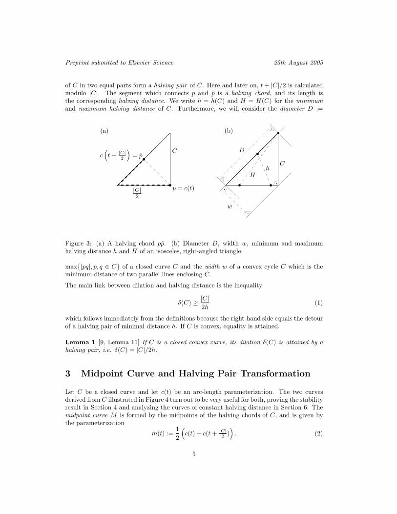
of C in two equal parts form a halving pair of C. Here and later on, t + |C|/2 is calculatedmodulo |C|. The segment which connects p and p is a halving chord, and its length isthe corresponding halving distance. We write h = h(C) and H = H(C) for the minimumand maximum halving distance of C. Furthermore, we will consider the diameter D :=

C

D

w

Hh

|C|2

p = c(t)

c(

t + |C|2

)

= pC

(a) (b)

Figure 3: (a) A halving chord pp. (b) Diameter D, width w, minimum and maximumhalving distance h and H of an isosceles, right-angled triangle.

max|pq|, p, q ∈ C of a closed curve C and the width w of a convex cycle C which is theminimum distance of two parallel lines enclosing C.

The main link between dilation and halving distance is the inequality

δ(C) ≥ |C|2h

(1)

which follows immediately from the definitions because the right-hand side equals the detourof a halving pair of minimal distance h. If C is convex, equality is attained.

Lemma 1 [9, Lemma 11] If C is a closed convex curve, its dilation δ(C) is attained by ahalving pair, i.e. δ(C) = |C|/2h.

3 Midpoint Curve and Halving Pair Transformation

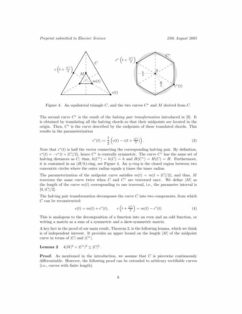
Let C be a closed curve and let c(t) be an arc-length parameterization. The two curvesderived from C illustrated in Figure 4 turn out to be very useful for both, proving the stabilityresult in Section 4 and analyzing the curves of constant halving distance in Section 6. Themidpoint curve M is formed by the midpoints of the halving chords of C, and is given bythe parameterization

m(t) :=1

2

(

c(t) + c(t + |C|2 ))

. (2)

5


C

M

C∗

h

2

H

2

c

(

t + |C|2

)

c(t)

m(t)c∗(t)

c∗(

t + |C|2

)

0

Figure 4: An equilateral triangle C, and the two curves C∗ and M derived from C.

The second curve C∗ is the result of the halving pair transformation introduced in [9]. Itis obtained by translating all the halving chords so that their midpoints are located in theorigin. Then, C∗ is the curve described by the endpoints of these translated chords. Thisresults in the parameterization

c∗(t) :=1

2

(

c(t) − c(t + |C|2 ))

. (3)

Note that c∗(t) is half the vector connecting the corresponding halving pair. By definition,c∗(t) = −c∗(t + |C|/2), hence C∗ is centrally symmetric. The curve C∗ has the same set ofhalving distances as C; thus, h(C∗) = h(C) = h and H(C∗) = H(C) = H . Furthermore,it is contained in an (H/h)-ring, see Figure 4. An η-ring is the closed region between twoconcentric circles where the outer radius equals η times the inner radius.

The parameterization of the midpoint curve satisfies m(t) = m(t + |C|/2), and thus, Mtraverses the same curve twice when C and C∗ are traversed once. We define |M | asthe length of the curve m(t) corresponding to one traversal, i.e., the parameter interval is[0, |C|/2].

The halving pair transformation decomposes the curve C into two components, from whichC can be reconstructed:

c(t) = m(t) + c∗(t), c(

t + |C|2

)

= m(t) − c∗(t) (4)

This is analogous to the decomposition of a function into an even and an odd function, orwriting a matrix as a sum of a symmetric and a skew-symmetric matrix.

A key fact in the proof of our main result, Theorem 2, is the following lemma, which we thinkis of independent interest. It provides an upper bound on the length |M | of the midpointcurve in terms of |C| and |C∗|.

Lemma 2 4|M |2 + |C∗|2 ≤ |C|2.

Proof. As mentioned in the introduction, we assume that C is piecewise continuouslydifferentiable. However, the following proof can be extended to arbitrary rectifiable curves(i.e., curves with finite length).

6


Using the linearity of the scalar product and |c(t)| = 1, we obtain

〈m(t), c∗(t)〉 (2),(3)=

1

4

⟨

c(t) + c(

t + |C|2

)

, c(t) − c(

t + |C|2

)⟩

(5)

=1

4

(

|c(t)|2 −∣∣∣c(

t + |C|2

)∣∣∣

2)

=1

4(1 − 1) = 0.

This means that the derivative vectors c∗(t) and m(t) are always orthogonal, thus (4) yields

|m(t)|2 + |c∗(t)|2 = |c(t)|2 = 1.

This implies

|C| =

∫ |C|

0

√

|m(t)|2 + |c∗(t)|2 dt

≥

√√√√

(∫ |C|

0

|m(t)| dt

)2

+

(∫ |C|

0

|c∗(t)| dt

)2

=

√

4 |M |2 + |C∗|2 (6)

The above inequality — from which the lemma follows — can be seen by a geometricargument: the left integral

∫ |C|

0

√

|m(t)|2 + |c∗(t)|2 dt

is the length of the curve

γ(s) :=

(∫ s

0

|m(t)| dt,

∫ s

0

|c∗(t)| dt

)

,

while the right expression√√√√

(∫ |C|

0

|m(t)| dt

)2

+

(∫ |C|

0

|c∗(t)| dt

)2

equals the distance of its end-points γ(0) = (0, 0) and γ (|C|).

Corollary 1 |C∗| ≤ |C|.

4 Stability Result for Closed Curves

In this section, we prove that a simple closed curve C of low dilation (close to π/2) is closeto being a circle. To this end, we first show that C∗ is close to a circle, i.e. H/h is close to 1.Then, we prove that the length of the midpoint curve is small. Combining both statementsyields the desired result.

We use the following lemma to find an upper bound on the ratio H/h. It extends aninequality of Ebbers-Baumann et al. [9, Theorem 22] to non-convex cycles.

7


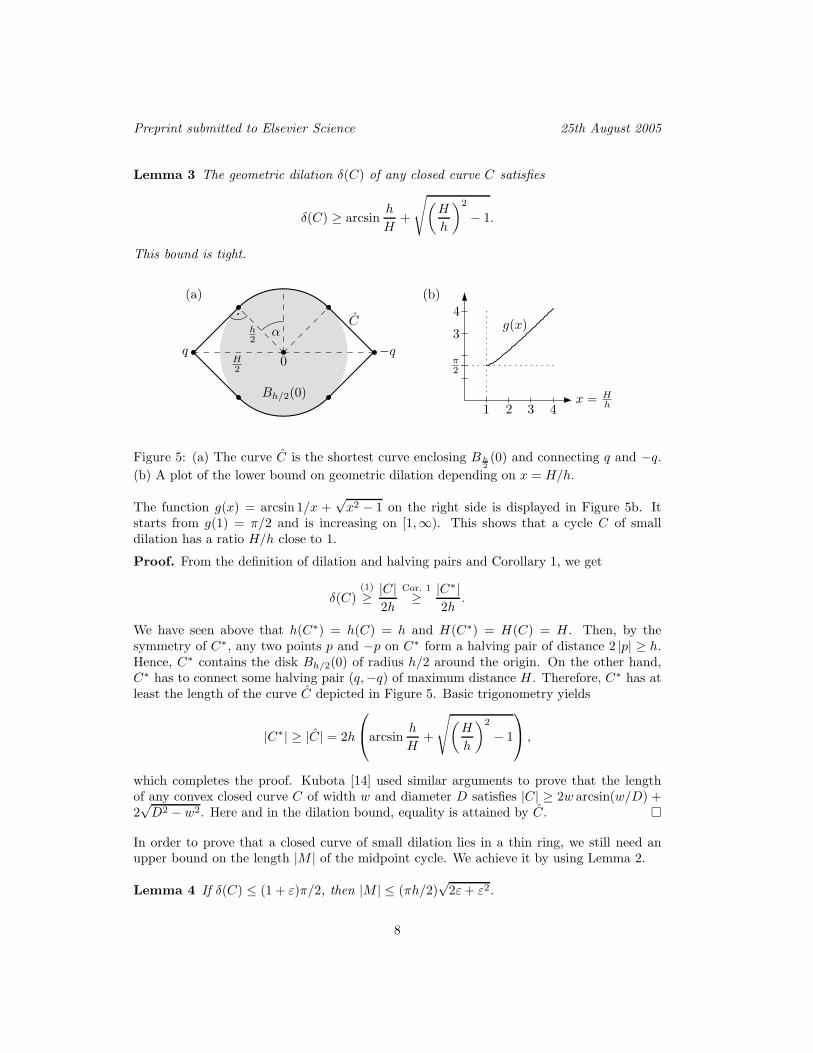
Lemma 3 The geometric dilation δ(C) of any closed curve C satisfies

δ(C) ≥ arcsinh

H+

√(

H

h

)2

− 1.

This bound is tight.

Bh/2(0)

h2

H2

α

q −q0

C

1 2 3 4

π2

x = Hh

g(x)3

4

(a) (b)

Figure 5: (a) The curve C is the shortest curve enclosing Bh

2

(0) and connecting q and −q.

(b) A plot of the lower bound on geometric dilation depending on x = H/h.

The function g(x) = arcsin 1/x +√

x2 − 1 on the right side is displayed in Figure 5b. Itstarts from g(1) = π/2 and is increasing on [1,∞). This shows that a cycle C of smalldilation has a ratio H/h close to 1.

Proof. From the definition of dilation and halving pairs and Corollary 1, we get

δ(C)(1)

≥ |C|2h

Cor. 1≥ |C∗|

2h.

We have seen above that h(C∗) = h(C) = h and H(C∗) = H(C) = H . Then, by thesymmetry of C∗, any two points p and −p on C∗ form a halving pair of distance 2 |p| ≥ h.Hence, C∗ contains the disk Bh/2(0) of radius h/2 around the origin. On the other hand,C∗ has to connect some halving pair (q,−q) of maximum distance H . Therefore, C∗ has atleast the length of the curve C depicted in Figure 5. Basic trigonometry yields

|C∗| ≥ |C| = 2h

arcsinh

H+

√(

H

h

)2

− 1

,

which completes the proof. Kubota [14] used similar arguments to prove that the lengthof any convex closed curve C of width w and diameter D satisfies |C| ≥ 2w arcsin(w/D) +2√

D2 − w2. Here and in the dilation bound, equality is attained by C.

In order to prove that a closed curve of small dilation lies in a thin ring, we still need anupper bound on the length |M | of the midpoint cycle. We achieve it by using Lemma 2.

Lemma 4 If δ(C) ≤ (1 + ε)π/2, then |M | ≤ (πh/2)√

2ε + ε2.

8


Proof. By the assumption and because the dilation of C is at least the detour of a halving

pair attaining minimum distance h, we have (1 + ε)π/2 ≥ δ(C)(1)

≥ |C|/2h, implying

|C| ≤ (1 + ε)πh. (7)

As seen before, C∗ encircles but does not enter the open disk Bh/2(0) of radius h/2 centeredat the origin 0. It follows that the length of C∗ is at least the perimeter of Bh/2(0):

|C∗| ≥ πh. (8)

By plugging everything together, we get

|M |Lemma 2

≤ 1

2

√

|C|2 − |C∗|2(7),(8)

≤ 1

2πh√

(1 + ε)2 − 1 =πh

2

√

2ε + ε2,

which concludes the proof of Lemma 4.

Intuitively it is clear (remember the definitions (2), (3) and Figure 4) that the upper boundon H/h from Lemma 3 and the upper bound on |M | of Lemma 4 imply that the curve Cis contained in a thin ring, if its dilation is close to π

2 . This is the idea behind Lemma 6,the main result of this section. To prove it, we will apply the following well-known fact, seee.g. [19], to M .

Lemma 5 Every closed curve C can be enclosed in a circle of radius |C|/4.

Proof. Fix a halving pair (p, p) of C. Then by definition, for any q ∈ C, we have |pq|+|qp| ≤dC(p, q) + dC(q, p) = dC(p, p) = |C|/2. It follows that C is contained in an ellipse with focip and p and major axis |C|/2. This ellipse is included in a circle with radius |C|/4, and thelemma follows.

Lemma 6 Let C ⊂ R2 be any simple closed curve with dilation δ(C) ≤ (1 + ε)π/2 forε ≤ 0.0001. Then C can be enclosed in a (1 + 3

√ε)-ring. This bound cannot be improved

apart from the coefficient of√

ε.

Proof. By Lemma 5, the midpoint cycle M can be enclosed in a circle of radius |M |/4 andsome center z. By the triangle inequality, we immediately obtain

|c(t) − z| (4)= |m(t) + c∗(t) − z| ≤ |c∗(t)| + |m(t) − z| ≤ H

2+

|M |4

,

|c(t) − z| (4)= |m(t) + c∗(t) − z| ≥ |c∗(t)| − |m(t) − z| ≥ h

2− |M |

4.

Thus, C can be enclosed in the ring between two concentric circles with radii R = H/2 +|M |/4 and r = h/2 − |M |/4 centered at z. To finish the proof, we have to bound theratio R/r. For simplicity, we prove only the asymptotic bound R/r ≤ 1+O(

√ε). The proof

of the precise bound, which includes all numerical estimates, is given in Appendix A.

9


Assume H/h = (1 + β). Lemma 3 and power series expansion yield the approximate lowerbound

δ(C) ≥ arcsin1

1 + β+√

(1 + β)2 − 1 =π

2+

2√

2

3β3/2 − O(β5/2). (9)

With our initial assumption δ(C) ≤ π2 (1+ε) we get therefore β = O(ε2/3). Lemma 4 implies

|M | = O(h√

ε) which yields

R

r=

H/2 + |M |/4

h/2 − |M |/4=

h(1 + β) + |M |/2

h − |M |/2≤ 1 + O(ε2/3) + O(ε1/2)

1 − O(ε1/2)= 1 + O(ε1/2),

completing the proof of the asymptotic bound in Lemma 6.

The lemma can be extended to a larger, more practical range of ε, by increasing the coeffi-cient of

√ε.

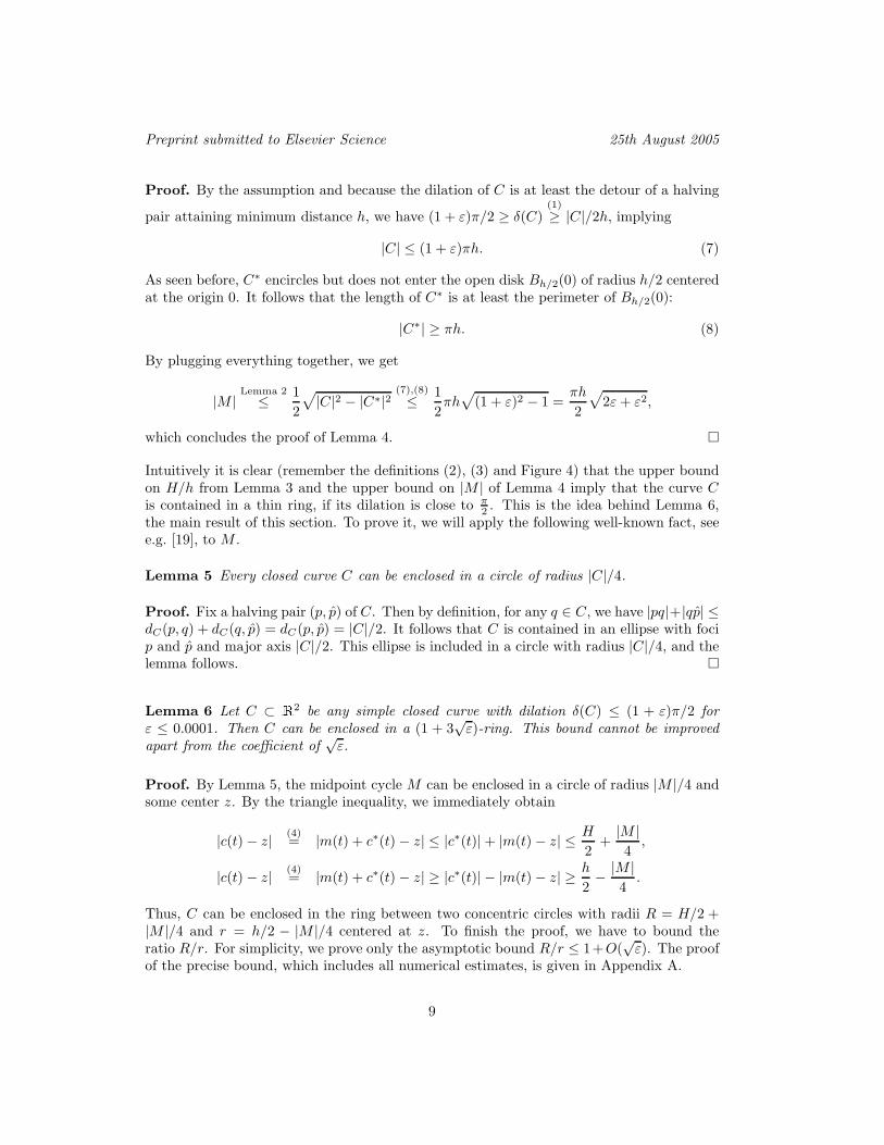
Tightness of the bound in Lemma 6. The curve C defined by the parameterization

ϕ

C

10

Figure 6: A moon’s orbit; the figure shows the curve C for s = 0.1.

c(ϕ) below and illustrated in Figure 6 shows that the order of magnitude in the boundcannot be improved. Note that c(ϕ) is not an arc-length parameterization.

c(ϕ) :=

(cos ϕ

sin ϕ

)

(1 + s cos 3ϕ) +

(− sin ϕ

cos ϕ

)

(−s

3sin 3ϕ).

This curve is the path of a moon moving around the earth on a small elliptic orbit withmajor axis 2s (collinear to the line earth–sun), with a frequency three times that of theearth’s own circular orbit around the sun.

Here, we only sketch how to bound the dilation and halving distances of this curve. Thedetails are given in Appendix B. A ring with outer radius R and inner radius r containing thecurve satisfies R/r ≥ (1+s)/(1−s) = 1+Θ(s). One can show that the length is bounded by|C| ≤ 2π+O(s2), and the halving distances are bounded by 2−O(s3) ≤ h < H ≤ 2+O(s3).

10


If s is not too large, C is convex, and this implies by Lemma 1 that the dilation is given by

δ(C) =|C|/2

h≤ π + O(s2)

2 − O(s3)= (1 + O(s2))

π

2.

Thus, we have dilation δ = (1 + ε)π/2 with ε = O(s2), but the ratio of the radii of theenclosing ring is 1 + Θ(s) = 1 + Ω(

√ε). A more careful estimate shows that this ratio is

1 + 32

√ε + O(ε). Thus, the coefficient 3 in Lemma 6 cannot be improved very much.

5 Improved Lower Bound on the Dilation of Finite Point

Sets

We now combine Lemma 6 with a disk packing result to achieve the desired new lowerbound on ∆. A (finite or infinite) set D of disks in the plane with disjoint interiors is calleda packing.

Theorem 1 (Kuperberg, Kuperberg, Matousek and Valtr [15]) Let D be a packing in theplane with circular disks of radius at most 1. Consider the set of disks D′ in which each diskD ∈ D is enlarged by a factor of Λ = 1.00001 from its center. Then D′ covers no squarewith side length 4.

There seems to be an overlooked case in the proof of this theorem given in [15]. (Usingthe terminology of [15], one of the conditions that needs to be checked in order to ensurethat Rn+1 is contained in Rn has been forgotten, see for example the disk D in Figure 11of [15].) We think that the proof can be fixed, and moreover, the result can be proved forvalues somewhat larger than 1.00001, as the authors did not try to optimize the constant Λ.However, the case distinctions are very delicate, and we have not fully worked out the detailsyet. For these reasons, we state our main result depending on the value Λ.

Theorem 2 Suppose Theorem 1 is true for a factor Λ with Λ ≤ 1.03. Then, the minimumgeometric dilation ∆ necessary to embed any finite set of points in the plane satisfies

∆ ≥ ∆(Λ) :=

(

1 +

(Λ − 1

3

)2)

π

2.

If Theorem 1 holds with Λ = 1.00001, this results in ∆ ≥ (1 + (10−10)/9)π/2 > (1 +10−11)π/2.

Proof. We first give an overview of the proof, and present the details afterwards. Considerthe set P := (x, y) | x, y ∈ −9,−8, . . . , 9 of grid points with integer coordinates in thesquare Q1 := [−9, 9]2 ⊂ R2 , see Figure 7. We use a proof by contradiction and assumethat there exists a planar connected graph G that contains P (as vertices or on its edges)and satisfies δ(G) < ∆(Λ). The idea of the proof is to show that if G attains such alow dilation, it contains a collection M of cycles with disjoint interiors which cover the

11


P

Q1

Q2

(−9,−9) (9,−9)

(9, 9)(−9, 9) (b)

xS

pq

1

1

C

(a)

ξ(p, q)

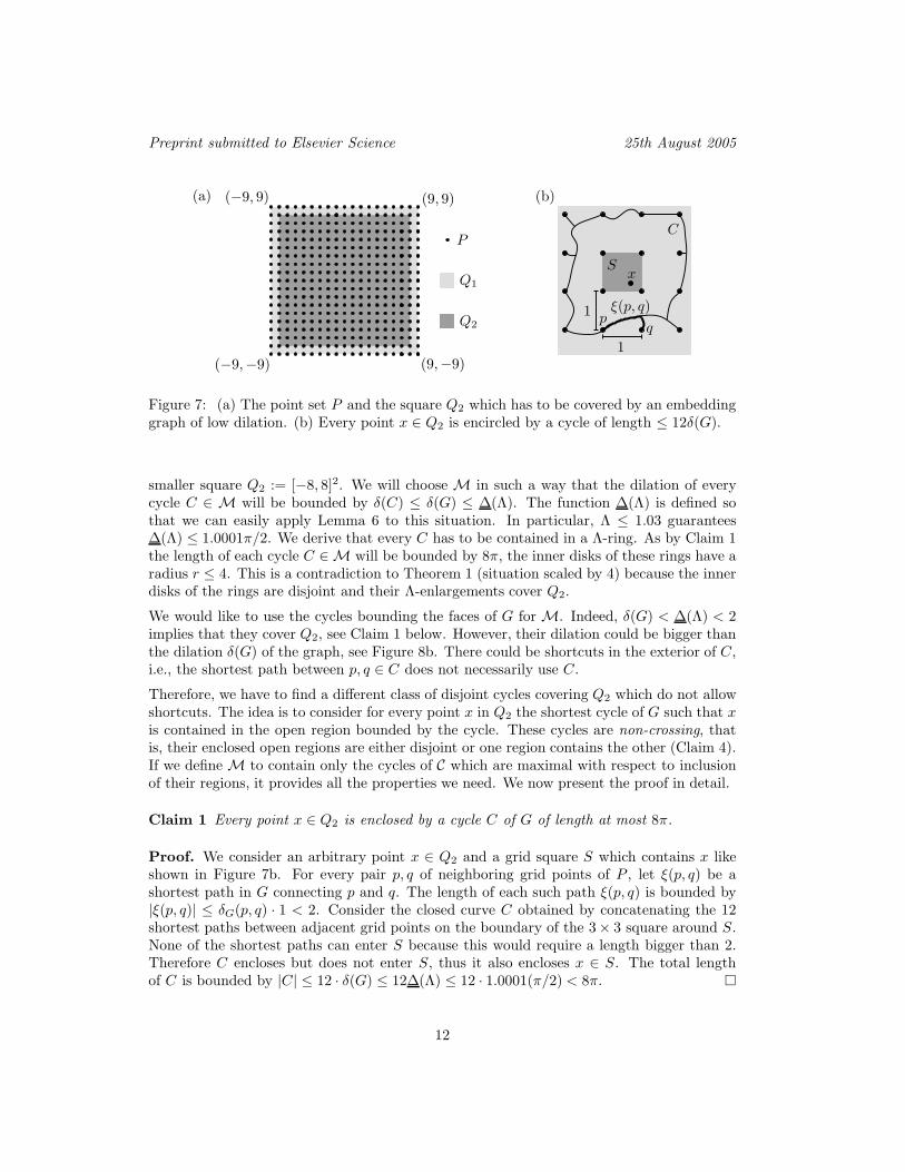
Figure 7: (a) The point set P and the square Q2 which has to be covered by an embeddinggraph of low dilation. (b) Every point x ∈ Q2 is encircled by a cycle of length ≤ 12δ(G).

smaller square Q2 := [−8, 8]2. We will choose M in such a way that the dilation of everycycle C ∈ M will be bounded by δ(C) ≤ δ(G) ≤ ∆(Λ). The function ∆(Λ) is defined sothat we can easily apply Lemma 6 to this situation. In particular, Λ ≤ 1.03 guarantees∆(Λ) ≤ 1.0001π/2. We derive that every C has to be contained in a Λ-ring. As by Claim 1the length of each cycle C ∈ M will be bounded by 8π, the inner disks of these rings have aradius r ≤ 4. This is a contradiction to Theorem 1 (situation scaled by 4) because the innerdisks of the rings are disjoint and their Λ-enlargements cover Q2.

We would like to use the cycles bounding the faces of G for M. Indeed, δ(G) < ∆(Λ) < 2implies that they cover Q2, see Claim 1 below. However, their dilation could be bigger thanthe dilation δ(G) of the graph, see Figure 8b. There could be shortcuts in the exterior of C,i.e., the shortest path between p, q ∈ C does not necessarily use C.

Therefore, we have to find a different class of disjoint cycles covering Q2 which do not allowshortcuts. The idea is to consider for every point x in Q2 the shortest cycle of G such that xis contained in the open region bounded by the cycle. These cycles are non-crossing, thatis, their enclosed open regions are either disjoint or one region contains the other (Claim 4).If we define M to contain only the cycles of C which are maximal with respect to inclusionof their regions, it provides all the properties we need. We now present the proof in detail.

Claim 1 Every point x ∈ Q2 is enclosed by a cycle C of G of length at most 8π.

Proof. We consider an arbitrary point x ∈ Q2 and a grid square S which contains x likeshown in Figure 7b. For every pair p, q of neighboring grid points of P , let ξ(p, q) be ashortest path in G connecting p and q. The length of each such path ξ(p, q) is bounded by|ξ(p, q)| ≤ δG(p, q) · 1 < 2. Consider the closed curve C obtained by concatenating the 12shortest paths between adjacent grid points on the boundary of the 3 × 3 square around S.None of the shortest paths can enter S because this would require a length bigger than 2.Therefore C encloses but does not enter S, thus it also encloses x ∈ S. The total lengthof C is bounded by |C| ≤ 12 · δ(G) ≤ 12∆(Λ) ≤ 12 · 1.0001(π/2) < 8π.

12


For any point x ∈ Q2, let C(x) denote a shortest cycle in G such that x is contained in theopen region bounded by the cycle. If the shortest cycle is not unique, we pick one whichencloses the smallest area. It follows from Claim 4 below that this defines the shortestcycle C(x) uniquely, but this fact is not essential for the proof. Obviously, C(x) is a simplecycle (i.e., without self-intersections). Let R(x) denote the open region enclosed by C(x).

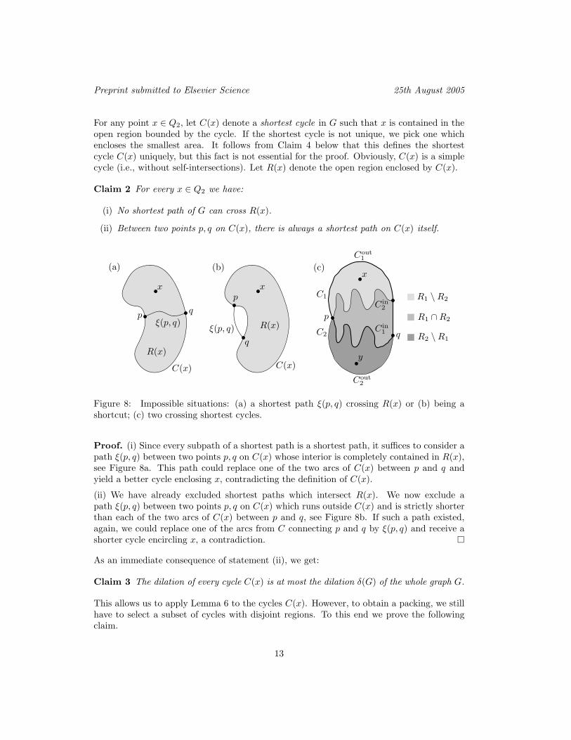
Claim 2 For every x ∈ Q2 we have:

(i) No shortest path of G can cross R(x).

(ii) Between two points p, q on C(x), there is always a shortest path on C(x) itself.

ξ(p, q)p

q

x

C(x)

ξ(p, q)

p

q

x

C(x)

R(x)

(a) (b)

C1

C2

C in

2

Cout

2

Cout

1

C in

1

(c)

R1 \ R2

R2 \ R1

R1 ∩ R2

R(x)

p

q

x

y

Figure 8: Impossible situations: (a) a shortest path ξ(p, q) crossing R(x) or (b) being ashortcut; (c) two crossing shortest cycles.

Proof. (i) Since every subpath of a shortest path is a shortest path, it suffices to consider apath ξ(p, q) between two points p, q on C(x) whose interior is completely contained in R(x),see Figure 8a. This path could replace one of the two arcs of C(x) between p and q andyield a better cycle enclosing x, contradicting the definition of C(x).

(ii) We have already excluded shortest paths which intersect R(x). We now exclude apath ξ(p, q) between two points p, q on C(x) which runs outside C(x) and is strictly shorterthan each of the two arcs of C(x) between p and q, see Figure 8b. If such a path existed,again, we could replace one of the arcs from C connecting p and q by ξ(p, q) and receive ashorter cycle encircling x, a contradiction.

As an immediate consequence of statement (ii), we get:

Claim 3 The dilation of every cycle C(x) is at most the dilation δ(G) of the whole graph G.

This allows us to apply Lemma 6 to the cycles C(x). However, to obtain a packing, we stillhave to select a subset of cycles with disjoint regions. To this end we prove the followingclaim.

13


Claim 4 For arbitrary points x, y ∈ Q2, the cycles C(x) and C(y) are non-crossing, i.e.,R(x) ∩ R(y) = ∅ ∨ R(x) ⊆ R(y) ∨ R(x) ⊆ R(y).

Proof. We argue by contradiction, see Figure 8c. Assume that the regions R1 and R2 ofthe shortest cycles C1 := C(x) and C2 := C(y) overlap, but none is fully contained insidethe other. This implies that their union R1 ∪ R2 is a bounded open connected set. Itsboundary ∂(R1 ∪ R2) contains a simple cycle C enclosing R1 ∪ R2.

By the assumptions we know that there is a part C in1 of C1 which connects two points p, q ∈

C2 and is, apart from its endpoints, completely contained in R2. Let Cout1 denote the other

path on C1 connecting p and q. By Claim 2(i), at least one of the paths C in1 or Cout

1 mustbe a shortest path. By Claim 2(ii), C in

1 cannot be a shortest path, since it intersects R2.Hence, only Cout

1 is a shortest path, implying |Cout1 | < |C1| /2. Analogously, we can split

C2 into two paths C in2 and Cout

2 such that C in2 is contained in R1, apart from its endpoints,

and |Cout2 | < |C2| /2.

The boundary cycle C consists of parts of C1 and parts of C2. It cannot contain any partof C in

1 or C in2 because it intersects neither with R1 nor with R2. Hence |C| ≤ |Cout

1 |+|Cout2 | <

(|C1|+ |C2|)/2 ≤ max|C1| , |C2|. Since C encloses x ∈ R1 and y ∈ R2, this contradicts thechoice of C1 = C(x) or C2 = C(y).

Let C be the set of shortest cycles C = C(x) | x ∈ Q2 , and let M ⊂ C be the set of maximalshortest cycles with respect to inclusion of their regions. Claim 4 implies that these cycleshave disjoint interiors and that they cover Q2. Claim 1 proves that their in-radius is boundedby r ≤ 4. By Claim 3, the dilation of every cycle C ∈ M satisfies δ(C) ≤ δ(G) ≤ ∆(Λ).Like described in the beginning of this proof we get a contradiction to Theorem 1. Thiscompletes the proof of the new lower bound (Theorem 2).

6 Closed Curves of Constant Halving Distance

Closed curves of constant halving distance turn up naturally if one wants to construct graphsof low dilation. Lemma 1 shows that the dilation of a convex curve of constant halvingdistance is attained by all its halving pairs. Hence, it is difficult to improve (decrease) thedilation of such cycles, because local changes decrease h or increase |C|.This is the motivation for using the curve of constant halving distance CF of Figure 9b toconstruct the grid of low dilation in Figure 2. Although the non-convex parts increase thelength and thereby the dilation of the small flowers CF , they are useful in decreasing thedilation of the big faces of the graph.

The proof of Lemma 6 shows that only curves with constant midpoint m(t) and constanthalving distance can attain the global dilation minimum of π/2. Furthermore, it shows thatonly circles satisfy both conditions; see also [9, Corollary 23], [1, Corollary 3.3], [16], [13].What happens if only one of the conditions is satisfied? Clearly, m(t) is constant if and onlyif C is centrally symmetric. On the other hand, the class of closed curves of constant halvingdistance is not as easy to describe. One could guess — incorrectly — that it consists only

14


C

M

30

p = (0, 12 )

p = (0,− 12 )

60

CF

M rR

h(CF )2

R

(a) (b)

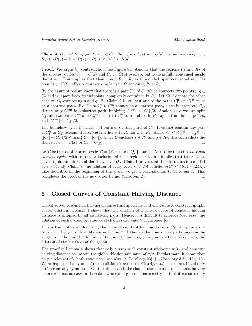
Figure 9: The “Rounded Triangle” C and the “Flower” CF are curves of constant halvingdistance.

of circles. The “Rounded Triangle” C shown in Figure 9a is a convex counterexample,and could be seen as an analog of the Reuleaux triangle, the best-known representative ofcurves of constant width [4]. It seems to be a somehow prominent example, because twogroups of the authors of this paper discovered it independently, before finding it in a paperof H. Auerbach [3, p. 141] from 1938.

We construct C by starting with a pair of points p := (0, 0.5) and p := (0,−0.5). Next,we move p to the right along a horizontal line. Simultaneously, p moves to the left suchthat the distance |pp| = 1 is preserved and both points move with equal speed. It can beshown that these conditions lead to a differential equation whose solution defines the pathof p uniquely. We move p and p like this until the connecting line segment pp forms an angleof 30 with the y-axis. Next, we swap the roles of p and p. Now, p moves along a line withthe direction of its last movement, and p moves with equal speed on the unique curve whichguarantees |pp| = 1, until pp has rotated with another 60. Again, we swap the roles of pand p for the next 60 and so forth. In this way we end up with six pieces of equal length(three straight line segments and three curved pieces) to build the Rounded Triangle Cdepicted in Figure 9a. Note that the rounded pieces are not parts of circles.

The details of the differential equation and its solution are given in Appendix C. Here, wemention only that the perimeter of C equals 3 ln 3. By Lemma 1 this results in

δ(C) = |C|/(2h(C)) =3

2ln 3 ≈ 1.6479 .

The midpoint curve of C is built from six congruent pieces that are arcs of a tractrix, aswe will discuss in the end of this section. First, we give a necessary and sufficient conditionfor curves of constant halving distance (not necessarily convex).

15


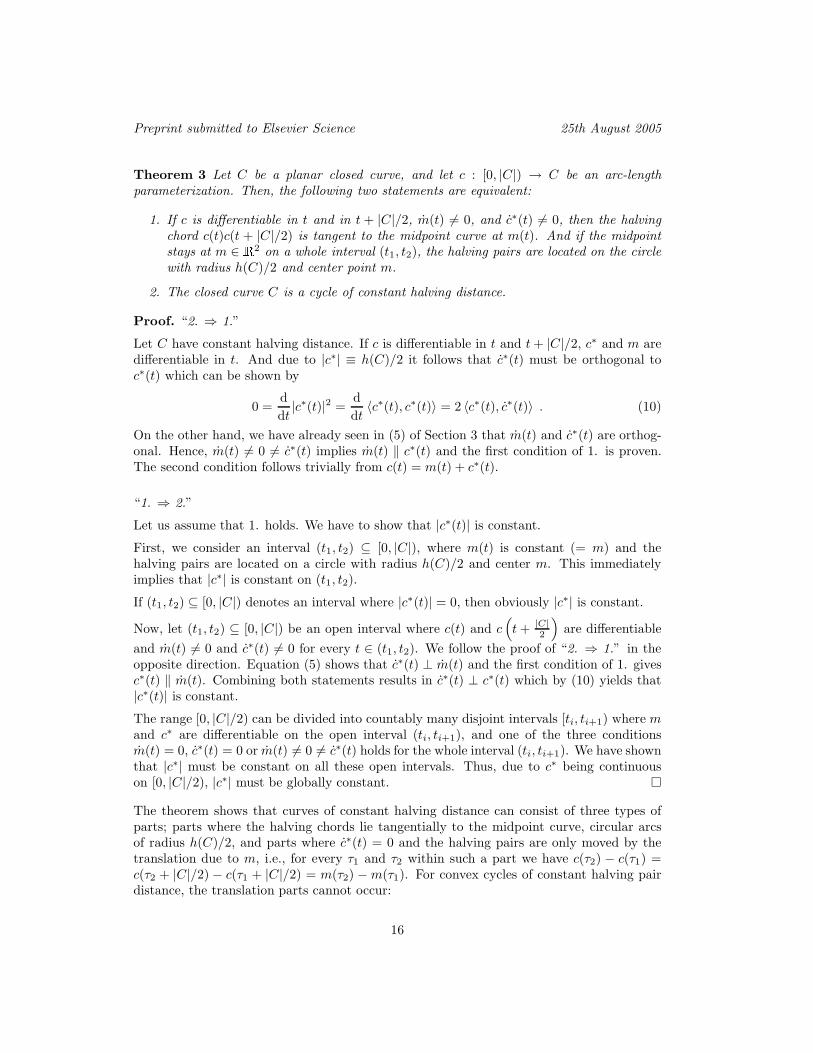
Theorem 3 Let C be a planar closed curve, and let c : [0, |C|) → C be an arc-lengthparameterization. Then, the following two statements are equivalent:

1. If c is differentiable in t and in t + |C|/2, m(t) 6= 0, and c∗(t) 6= 0, then the halvingchord c(t)c(t + |C|/2) is tangent to the midpoint curve at m(t). And if the midpointstays at m ∈ R2 on a whole interval (t1, t2), the halving pairs are located on the circlewith radius h(C)/2 and center point m.

2. The closed curve C is a cycle of constant halving distance.

Proof. “2. ⇒ 1.”

Let C have constant halving distance. If c is differentiable in t and t + |C|/2, c∗ and m aredifferentiable in t. And due to |c∗| ≡ h(C)/2 it follows that c∗(t) must be orthogonal toc∗(t) which can be shown by

0 =d

dt|c∗(t)|2 =

d

dt〈c∗(t), c∗(t)〉 = 2 〈c∗(t), c∗(t)〉 . (10)

On the other hand, we have already seen in (5) of Section 3 that m(t) and c∗(t) are orthog-onal. Hence, m(t) 6= 0 6= c∗(t) implies m(t) ‖ c∗(t) and the first condition of 1. is proven.The second condition follows trivially from c(t) = m(t) + c∗(t).

“1. ⇒ 2.”

Let us assume that 1. holds. We have to show that |c∗(t)| is constant.

First, we consider an interval (t1, t2) ⊆ [0, |C|), where m(t) is constant (= m) and thehalving pairs are located on a circle with radius h(C)/2 and center m. This immediatelyimplies that |c∗| is constant on (t1, t2).

If (t1, t2) ⊆ [0, |C|) denotes an interval where |c∗(t)| = 0, then obviously |c∗| is constant.

Now, let (t1, t2) ⊆ [0, |C|) be an open interval where c(t) and c(

t + |C|2

)

are differentiable

and m(t) 6= 0 and c∗(t) 6= 0 for every t ∈ (t1, t2). We follow the proof of “2. ⇒ 1.” in theopposite direction. Equation (5) shows that c∗(t) ⊥ m(t) and the first condition of 1. givesc∗(t) ‖ m(t). Combining both statements results in c∗(t) ⊥ c∗(t) which by (10) yields that|c∗(t)| is constant.

The range [0, |C|/2) can be divided into countably many disjoint intervals [ti, ti+1) where mand c∗ are differentiable on the open interval (ti, ti+1), and one of the three conditionsm(t) = 0, c∗(t) = 0 or m(t) 6= 0 6= c∗(t) holds for the whole interval (ti, ti+1). We have shownthat |c∗| must be constant on all these open intervals. Thus, due to c∗ being continuouson [0, |C|/2), |c∗| must be globally constant.

The theorem shows that curves of constant halving distance can consist of three types ofparts; parts where the halving chords lie tangentially to the midpoint curve, circular arcsof radius h(C)/2, and parts where c∗(t) = 0 and the halving pairs are only moved by thetranslation due to m, i.e., for every τ1 and τ2 within such a part we have c(τ2) − c(τ1) =c(τ2 + |C|/2) − c(τ1 + |C|/2) = m(τ2) − m(τ1). For convex cycles of constant halving pairdistance, the translation parts cannot occur:

16


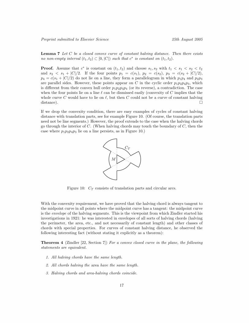
Lemma 7 Let C be a closed convex curve of constant halving distance. Then there existsno non-empty interval (t1, t2) ⊂ [0, |C|) such that c∗ is constant on (t1, t2).

Proof. Assume that c∗ is constant on (t1, t2) and choose s1, s2 with t1 < s1 < s2 < t2and s2 < s1 + |C|/2. If the four points p1 = c(s1), p2 = c(s2), p3 = c(s2 + |C|/2),p4 = c(s1 + |C|/2) do not lie on a line, they form a parallelogram in which p1p4 and p2p3

are parallel sides. However, these points appear on C in the cyclic order p1p2p4p3, whichis different from their convex hull order p1p2p3p4 (or its reverse), a contradiction. The casewhen the four points lie on a line ℓ can be dismissed easily (convexity of C implies that thewhole curve C would have to lie on ℓ, but then C could not be a curve of constant halvingdistance).

If we drop the convexity condition, there are easy examples of cycles of constant halvingdistance with translation parts, see for example Figure 10. (Of course, the translation partsneed not be line segments.) However, the proof extends to the case when the halving chordsgo through the interior of C. (When halving chords may touch the boundary of C, then thecase where p1p2p4p3 lie on a line persists, as in Figure 10.)

CT

M

Figure 10: CT consists of translation parts and circular arcs.

With the convexity requirement, we have proved that the halving chord is always tangent tothe midpoint curve in all points where the midpoint curve has a tangent: the midpoint curveis the envelope of the halving segments. This is the viewpoint from which Zindler started hisinvestigations in 1921: he was interested in envelopes of all sorts of halving chords (halvingthe perimeter, the area, etc., and not necessarily of constant length) and other classes ofchords with special properties. For curves of constant halving distance, he observed thefollowing interesting fact (without stating it explicitly as a theorem):

Theorem 4 (Zindler [22, Section 7]) For a convex closed curve in the plane, the followingstatements are equivalent.

1. All halving chords have the same length.

2. All chords halving the area have the same length.

3. Halving chords and area-halving chords coincide.

17


Following Auerbach [3], these curves are consequently called Zindler curves. (The theoremholds also for non-convex curves as long as all halving chords go through the interior of C, andit remains even true for chords that divide the area or perimeter in some arbitrary constantratio.) Auerbach [3] noted than these curves are related to a problem of S. Ulam aboutfloating bodies. Ulam’s original problem [18, Problem 19, pp. 90–92], [5, Section A6, p. 19–20], [20, pp. 153–154], which is still unsolved in its generality, asks if there is a homogeneousbody different from a spherical ball that can float in equilibrium in any orientation. A two-dimensional version can be formulated as follows: consider a homogeneous cylindrical log ofdensity 1

2 whose cross-section is a convex curve C, floating in water (which has density 1).This log will float in equilibrium with respect to rolling in every horizontal position if andonly if C is a Zindler curve.

Moreover, Auerbach relates these curves to curves of constant width [4, § 7]:

Theorem 5 (Auerbach [3]) If a square PQRS moves rigidly in the plane such the diagonalPR traces all halving chords of a Zindler curve C the endpoints of the other diagonal QStrace out a curve D of constant width, enclosing the same area as C.

Conversely, one can start from any curve of constant width. Taking point pairs Q and Swith parallel tangents as diagonals of squares PQRS, the other diagonal PR will generatea curve of constant halving distance, not necessarily convex. Theorem 5 remains true for arhombus PQRS as long as QS is it not too short, relatively to PR. (Of course, the area ofD will then be different.)

−2 −1 1 2

−0.4

0.8

1.2

tractrix

end of chain

watchchain

watch

edge of table

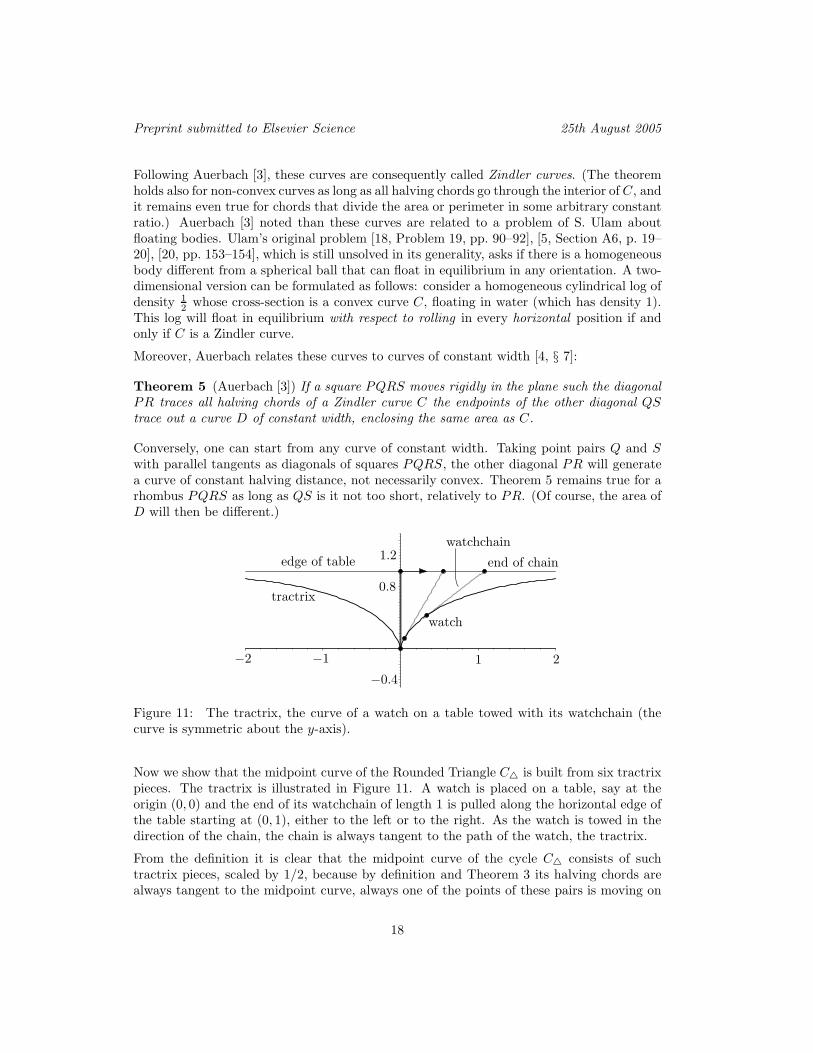
Figure 11: The tractrix, the curve of a watch on a table towed with its watchchain (thecurve is symmetric about the y-axis).

Now we show that the midpoint curve of the Rounded Triangle C is built from six tractrixpieces. The tractrix is illustrated in Figure 11. A watch is placed on a table, say at theorigin (0, 0) and the end of its watchchain of length 1 is pulled along the horizontal edge ofthe table starting at (0, 1), either to the left or to the right. As the watch is towed in thedirection of the chain, the chain is always tangent to the path of the watch, the tractrix.

From the definition it is clear that the midpoint curve of the cycle C consists of suchtractrix pieces, scaled by 1/2, because by definition and Theorem 3 its halving chords arealways tangent to the midpoint curve, always one of the points of these pairs is moving on

18


a straight line, and its distance to the midpoint curve stays 1/2. A parameterization notdepending on the midpoint curve is analyzed in Appendix C.

As mentioned in the introduction, Zindler [22, Section 7.b] discovered some convex curvesof constant halving distance already in 1921. He restricted his analysis to curves whosemidpoint curves have three cusps like the one of the rounded triangle. His example uses asthe midpoint curve the path of a point on a circle of radius 1 rolling inside of a bigger circleof radius 3 (a hypocycloid). To guarantee convexity, one then needs h ≥ 48.

7 Relating Halving Distance to other Geometric Quan-

tities

One important topic in convex geometry is the relation between different geometric quan-tities of convex bodies like area A and diameter D. Scott and Awyong [19] give a shortsurvey of basic inequalities in R2. For example, it is known that 4A ≤ πD2, and equality isattained only by circles, the so-called extremal set of this inequality.

In this context the minimum and maximum halving distance h and H give rise to somenew interesting questions, namely the relation to other basic quantities like the width w.As the inequality h ≤ w is immediate from definition, the known upper bounds on w holdfor h as well. However, although the original inequalities relating w to perimeter, diameter,area, inradius and circumradius are tight (see [19]), not all of them are also tight for h. Onecounterexample (A ≥ w2/

√3 ≥ h2/

√3) will be discussed in the following subsection.

7.1 Minimum Halving Distance and Area

Here, we consider the relation of the minimum halving distance h and the area A. Clearly,the area can get arbitrarily big while h stays constant. For instance this is the case for arectangle of smaller side length h where the bigger side length tends to infinity.

How small the area A can get for closed convex curves of minimum halving distance h? A firstanswer A ≥ h2/

√3 is easy to prove, because it is known [21, ex. 6.4, p.221] that A ≥ w2/

√3,

and we combine this with w ≥ h. Still, 1/√

3 ≈ 0.577 is not the best possible lower boundto A/h2, since the equilateral triangle is the only closed curve attaining A = w2/

√3 and

its width w =√

3/2 ≈ 0.866 (for side length 1) is strictly bigger than its minimum halvingdistance h = 3/4 = 0.75. We do not know the smallest possible value of A/h2.

We can also consider chords bisecting the area of planar convex sets instead of halving theirperimeter, see [5, Section A26, p. 37] about “dividing up a piece of land by a short fence”.Let harea be the minimum area-halving distance. Santalo asked5 if A ≥ (π/4)h2

area. Equalityis attained by a circle.

Now going back to perimeter halving distance, does the circle attain smallest area for a

given h? Already the equilateral triangle gives a counterexample, A/h2 =√

34 / 9

16 ≈ 0.770 <

5We would like to thank Salvador Segura Gomis for pointing this out.

19


1

1

1

2

1

2

√

3

2

harea =1√

2

h =3

4

A =

√

3

4h = harea = 2

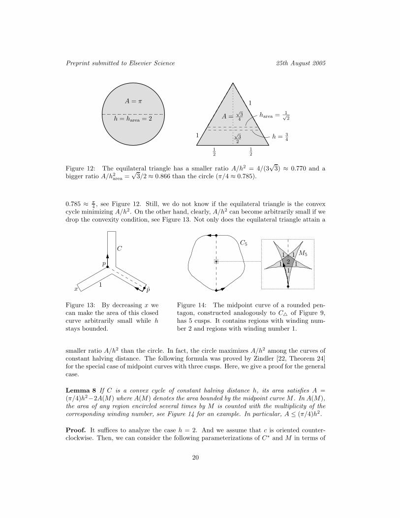
A = π

Figure 12: The equilateral triangle has a smaller ratio A/h2 = 4/(3√

3) ≈ 0.770 and abigger ratio A/h2

area =√

3/2 ≈ 0.866 than the circle (π/4 ≈ 0.785).

0.785 ≈ π4 , see Figure 12. Still, we do not know if the equilateral triangle is the convex

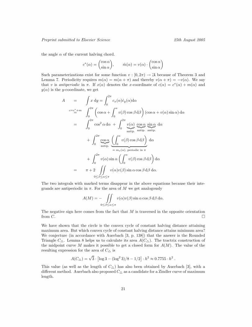
cycle minimizing A/h2. On the other hand, clearly, A/h2 can become arbitrarily small if wedrop the convexity condition, see Figure 13. Not only does the equilateral triangle attain a

C

p

px1

Figure 13: By decreasing x wecan make the area of this closedcurve arbitrarily small while hstays bounded.

C5

21

M5

1

1

1 1

Figure 14: The midpoint curve of a rounded pen-tagon, constructed analogously to C of Figure 9,has 5 cusps. It contains regions with winding num-ber 2 and regions with winding number 1.

smaller ratio A/h2 than the circle. In fact, the circle maximizes A/h2 among the curves ofconstant halving distance. The following formula was proved by Zindler [22, Theorem 24]for the special case of midpoint curves with three cusps. Here, we give a proof for the generalcase.

Lemma 8 If C is a convex cycle of constant halving distance h, its area satisfies A =(π/4)h2−2A(M) where A(M) denotes the area bounded by the midpoint curve M . In A(M),the area of any region encircled several times by M is counted with the multiplicity of thecorresponding winding number, see Figure 14 for an example. In particular, A ≤ (π/4)h2.

Proof. It suffices to analyze the case h = 2. And we assume that c is oriented counter-clockwise. Then, we can consider the following parameterizations of C∗ and M in terms of

20


the angle α of the current halving chord.

c∗(α) =

(cos α

sin α

)

, m(α) = v(α) ·(

cos α

sin α

)

Such parameterizations exist for some function v : [0, 2π) → R because of Theorem 3 andLemma 7. Periodicity requires m(α) = m(α + π) and thereby v(α + π) = −v(α). We saythat v is antiperiodic in π. If x(α) denotes the x-coordinate of c(α) = c∗(α) + m(α) andy(α) is the y-coordinate, we get

A =

∫

x dy =

∫ 2π

0

cx(α)cy(α)dα

c=c∗+m=

∫ 2π

0

(

cos α +

∫ α

0

v(β) cos β dβ

)

(cos α + v(α) sin α) dα

=

∫ 2π

0

cos2 α dα +

∫ 2π

0

v(α)︸︷︷︸

antip.

cos α︸︷︷︸

antip.

sin α︸︷︷︸

antip.

dα

+

∫ 2π

0

cos α︸︷︷︸

antip.

(∫ α

0

v(β) cos β dβ

)

︸︷︷︸

= mx(α), periodic in π

dα

+

∫ 2π

0

v(α) sin α

(∫ α

0

v(β) cos β dβ

)

dα

= π + 2

∫∫

0≤β≤α≤π

v(α)v(β) sin α cos β dβ dα.

The two integrals with marked terms disappear in the above equations because their inte-grands are antiperiodic in π. For the area of M we get analogously

A(M) = −∫∫

0≤β≤α≤π

v(α)v(β) sin α cos β dβ dα.

The negative sign here comes from the fact that M is traversed in the opposite orientationfrom C.

We have shown that the circle is the convex cycle of constant halving distance attainingmaximum area. But which convex cycle of constant halving distance attains minimum area?We conjecture (in accordance with Auerbach [3, p. 138]) that the answer is the RoundedTriangle C. Lemma 8 helps us to calculate its area A(C). The tractrix construction ofthe midpoint curve M makes it possible to get a closed form for A(M). The value of theresulting expression for the area of C is

A(C) =√

3 ·[log 3 − (log2 3)/8 − 1/2

]· h2 ≈ 0.7755 · h2 .

This value (as well as the length of C) has also been obtained by Auerbach [3], with adifferent method. Auerbach also proposed C as a candidate for a Zindler curve of maximumlength.

21


Zindler’s curve [22, Section 7.b], which we described in the end of Section 6, has area ((π/4)−(1/24)2π)h2 ≈ 0.780h2. Both constant factors are smaller than π/4 ≈ 0.7854 . . ., thusproviding a negative answer to the above-mentioned question of Santalo whether A ≥(π/4)h2

area. It would be interesting to know whether C has the smallest area among allconvex curves with a given minimum area-halving distance harea.

Auerbach [3] constructed another, non-convex, curve of constant halving width, based on thesame tractrix construction as the rounded triangle C, but consisting of only two straightedges and two smooth arcs, forming the shape of a heart. Approximate renditions of bothcurves can be found in several problem collections [18, Fig. 19.1, p. 91], [5, Fig. A9, p. 20],[20, Figs. 179 and 180, pp. 153–154] and other popular books, but they appear to usecircular arcs instead of the correct boundary curves, given by the parametrization (19) inAppendix C.

7.2 Minimum Halving Distance and Width

In order to achieve a lower bound to h in terms of w, we examine the relation of bothquantities to the area A and the diameter D. The following inequality was first proved byKubota [14] in 1923 and is listed in [19].

Theorem 6 (Kubota [14]) If C is a convex curve, then A ≥ Dw/2.

We will combine this known inequality with the following new result.

Theorem 7 If C is a convex curve, then A ≤ Dh.

Proof. Without loss of generality we assume that a halving chord pp of minimum length hlies on the y-axis, p on top and p at the bottom, see Figure 15. Let C− be the part ofC with negative x-coordinate and let C+ := C \ C− be the remaining part. We have|C−| = |C+| = |C|/2 because pp is a halving chord. In Figure 15, obviously |C−| = |C+|does not hold, but this is only to illustrate our proof by contradiction. Let −x1 and x2

denote the minimum and maximum x-coordinate of C. Note that x1 has a positive value.We assume that x2 > x1. Otherwise we could reflect C at the y-axis. Let y(x) be thelength of the vertical line segment of x-coordinate x inside C, for every x ∈ [−x1, x2]. Thesedefinitions result in x1 + x2 ≤ D and A =

∫ x2

−x1

y(x) dx. Furthermore, if we take the convex

hull of the vertical segment with x-coordinate x and length y(x) and the vertical segmentwith x-coordinate −x and length y(−x), then its intersection with the y-axis has length(y(−x) + y(x))/2. By convexity it must be contained in the line segment pp of length h.This implies

∀x ∈ [0, x1] : y(−x) + y(x) ≤ 2h . (11)

As a next step, we want to show that

∀x ∈ [x1, x2] : y(x) ≤ h . (12)

We assume that y(x) > h. Let ab be the vertical segment of x-coordinate x inside C, a ontop and b at the bottom. Then, we consider the lines ℓ1 through p and a and ℓ2 through

22


h

y(x)

−x1 0 x1 x x2

ℓ1

ℓ2

p

p

a

b

L2

C

1

z

h

w

α

x

(b)(a)

L1

L1

L2

c

d

Figure 15: (a) Proving by contradiction that y(x) ≤ h for every x in [x1, x2]. (b) In a thinisosceles triangle h/w ց 1/2 if α → 0.

p and b. Let L1 (L2) be the length of the piece of ℓ1 (ℓ2) with x-coordinates in [0, x1]. Byconstruction they are equal to the corresponding lengths in the x-interval [−x1, 0]. Let cand d be the points with x-coordinate −x1 on ℓ1, ℓ2 respectively. Then, by the convexity ofC, we have |C−| ≤ L1 + L2 + |cd| ≤ L1 + L2 + h < L1 + L2 + y(x) ≤ |C+|. This contradictsto pp being a halving chord, and the proof of (12) is complete.

Now we can plug everything together and get

A =

x2∫

−x1

y(x) dx =

x1∫

0

(y(−x) + y(x)) dx +

x2∫

x1

y(x) dx

(11), (12)

≤ x1 · 2h + (x2 − x1)h = (x1 + x2)h ≤ Dh .

Finally, we achieve the desired inequality relating h and w.

Theorem 8 If C is a convex curve, then h ≥ w/2. This bound is tight.

Proof. The inequality follows directly from Theorem 6 and Theorem 7. To see that thebound is tight, consider a thin isosceles triangle like in Figure 15b. If h is the minimumhalving distance, we have 2z = |C|/2 = 1 + x/2 = 1 + sin(α/2), thus h = 2z sin α

2 = (1 +sin(α/2)) sin(α/2). On the other hand, the width is given by w = sin α = 2 sin(α/2) cos(α/2),therefore h/w = (1 + sin(α/2))/(2 cos(α/2)) ց 1/2 for α → 0.

Theorem 8 can be also proved directly by using arguments analogous to the proof of Theo-rem 7. But we think that Theorem 7 is of independent interest.

23


8 Dilation Bounds

8.1 Upper Bound on Geometric Dilation

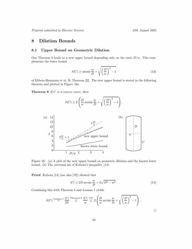
Our Theorem 8 leads to a new upper bound depending only on the ratio D/w. This com-plements the lower bound

δ(C) ≥ arcsinw

D+

√(

D

w

)2

− 1 (13)

of Ebbers-Baumann et al. [9, Theorem 22]. The new upper bound is stated in the followingtheorem and plotted in Figure 16a.

Theorem 9 If C is a convex curve, then

δ(C) ≤ 2

D

warcsin

w

D+

√(

D

w

)2

− 1

.

0

2

4

6

8

10

12

14

1 2 3 4D/w

known lower bound

new upper bound

π D

w

2D

w+ 1

δ

C

D

w

(a) (b)

Figure 16: (a) A plot of the new upper bound on geometric dilation and the known lowerbound. (b) The extremal set of Kubota’s inequality (14).

Proof. Kubota [14] (see also [19]) showed that

|C| ≤ 2D arcsinw

D+ 2√

D2 − w2 . (14)

Combining this with Theorem 8 and Lemma 1 yields

δ(C)Lemma 1

=|C|2h

Theorem 8≤ |C|

w

(14)

≤ 2

D

warcsin

w

D+

√(

D

w

)2

− 1

.

24


The isoperimetric inequality |C| ≤ Dπ and the inequality |C| ≤ 2D +2w lead to the slightlybigger but simpler dilation bounds δ(C) ≤ π D

w and δ(C) ≤ 2(

Dw + 1

), see Figure 16a. But

even the dilation bound of Theorem 9 is not tight because (14) becomes an equality only forcurves which result from the intersection of a circular disk of diameter D with a parallel stripof width w, see Figure 16b. For these curves we have h = w due to their central symmetry,but equality in our upper bound can only be attained for 2h = w.

8.2 Lower Bounds on the Geometric Dilation of Polygons

In this subsection we apply the lower bound (13) of Ebbers-Baumann et al. [9] to deducelower bounds on the dilation of polygons with n sides (in special cases we proceed directly).We start with the case of a triangle (and skip the easy proof):

Lemma 9 For any triangle C, δ(C) ≥ 2. This bound is tight.

Equality is attained by equilateral triangles. Note that plugging the inequality D/w ≥ 2/√

3into (13) would only give δ(C) ≥ π/3+1/

√3 ≈ 1.624. We continue with the case of centrally

symmetric convex polygons, for which we obtain a tight bound.

Theorem 10 If C is a centrally symmetric convex n-gon (thus n is even), then

δ(C) ≥ n

2tan

π

n.

This bound is tight.

Proof. We adapt the proof of Theorem 22 in [9], which proves inequality (13) for closedcurves. Since C is centrally symmetric, it must contain a circle of radius r = h/2. Itcan easily be shown (using the convexity of the tangent function) that the shortest n-goncontaining such a circle is a regular n-gon. Its length equals 2rn tan π/n which furtherimplies that

δ(C)Lemma 1

=|C|2h

≥ hn tan πn

2h=

n

2tan

π

n. (15)

The bound is tight for a regular n-gon.

In the last part of this section we address the case of arbitrary (not necessarily convex)polygons. Let C be a polygon with n vertices, and let C′ = conv(C). Clearly C′ has atmost n vertices. By Lemma 9 in [9], δ(C) ≥ δ(C′). Further on, consider

C′′ =C′ + (−C′)

2,

the convex curve obtained by central symmetrization from C′ (see [21, 9]). It is easy tocheck that C′′ is a convex polygon, whose number of vertices n′′ is even and at most twicethat of C′, therefore at most 2n. Because δ(C′′) ≤ δ(C′) by Lemma 16 in [9], we get

δ(C) ≥ δ(C′) ≥ δ(C′′)Theorem 10, n′′≤2n

≥ n tanπ

2n

and obtain a lower bound on the geometric dilation of any polygon with n sides.

25


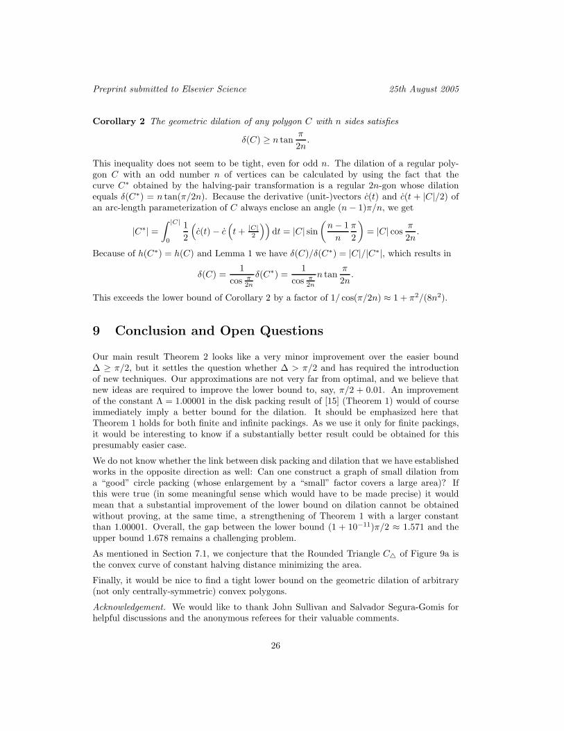
Corollary 2 The geometric dilation of any polygon C with n sides satisfies

δ(C) ≥ n tanπ

2n.

This inequality does not seem to be tight, even for odd n. The dilation of a regular poly-gon C with an odd number n of vertices can be calculated by using the fact that thecurve C∗ obtained by the halving-pair transformation is a regular 2n-gon whose dilationequals δ(C∗) = n tan(π/2n). Because the derivative (unit-)vectors c(t) and c(t + |C|/2) ofan arc-length parameterization of C always enclose an angle (n − 1)π/n, we get

|C∗| =

∫ |C|

0

1

2

(

c(t) − c(

t + |C|2

))

dt = |C| sin(

n − 1

n

π

2

)

= |C| cosπ

2n.

Because of h(C∗) = h(C) and Lemma 1 we have δ(C)/δ(C∗) = |C|/|C∗|, which results in

δ(C) =1

cos π2n

δ(C∗) =1

cos π2n

n tanπ

2n.

This exceeds the lower bound of Corollary 2 by a factor of 1/ cos(π/2n) ≈ 1 + π2/(8n2).

9 Conclusion and Open Questions

Our main result Theorem 2 looks like a very minor improvement over the easier bound∆ ≥ π/2, but it settles the question whether ∆ > π/2 and has required the introductionof new techniques. Our approximations are not very far from optimal, and we believe thatnew ideas are required to improve the lower bound to, say, π/2 + 0.01. An improvementof the constant Λ = 1.00001 in the disk packing result of [15] (Theorem 1) would of courseimmediately imply a better bound for the dilation. It should be emphasized here thatTheorem 1 holds for both finite and infinite packings. As we use it only for finite packings,it would be interesting to know if a substantially better result could be obtained for thispresumably easier case.

We do not know whether the link between disk packing and dilation that we have establishedworks in the opposite direction as well: Can one construct a graph of small dilation froma “good” circle packing (whose enlargement by a “small” factor covers a large area)? Ifthis were true (in some meaningful sense which would have to be made precise) it wouldmean that a substantial improvement of the lower bound on dilation cannot be obtainedwithout proving, at the same time, a strengthening of Theorem 1 with a larger constantthan 1.00001. Overall, the gap between the lower bound (1 + 10−11)π/2 ≈ 1.571 and theupper bound 1.678 remains a challenging problem.

As mentioned in Section 7.1, we conjecture that the Rounded Triangle C of Figure 9a isthe convex curve of constant halving distance minimizing the area.

Finally, it would be nice to find a tight lower bound on the geometric dilation of arbitrary(not only centrally-symmetric) convex polygons.

Acknowledgement. We would like to thank John Sullivan and Salvador Segura-Gomis forhelpful discussions and the anonymous referees for their valuable comments.

26


References

[1] A. Abrams, J. Cantarella, J. Fu, M. Ghomi, and R. Howard. Circles minimize mostknot energies. Topology, 42(2):381–394, 2002.

[2] P. K. Agarwal, R. Klein, C. Knauer, and M. Sharir. Computing the detour of polyg-onal curves. Technical report, Freie Universitat Berlin, Fachbereich Mathematik undInformatik, 2002.

[3] H. Auerbach. Sur un probleme de M. Ulam concernant l’equilibre des corps flottants.Studia Math., 7:121–142, 1938.

[4] G. D. Chakerian and H. Groemer. Convex bodies of constant width. In P. M. Gruberand J. M. Wills, editors, Convexity and its Applications, pp. 49–96. Birkhauser, Boston,1983.

[5] H. P. Croft, K. J. Falconer, and R. K. Guy. Unsolved Problems in Geometry. Springer-Verlag, 1991.

[6] A. Dumitrescu, A. Ebbers-Baumann, A. Grune, R. Klein, and G. Rote. On geometricdilation and halving chords. In Proc. 9th Worksh. Algorithms and Data Structures(WADS 2005), volume 3608 of Lecture Notes Comput. Sci. Springer, August 2005,pp. 244–255.

[7] A. Dumitrescu, A. Grune, and G. Rote. Improved lower bound on the geometric dila-tion of point sets. In Abstracts 21st European Workshop Comput. Geom., pp. 37–40.Technische Universiteit Eindhoven, 2005.

[8] A. Ebbers-Baumann, A. Grune, and R. Klein. On the geometric dilation of finite pointsets. In 14th Annual International Symposium on Algorithms and Computation, volume2906 of LNCS, pp. 250–259. Springer, 2003. Journal version to appear in Algorithmica.

[9] A. Ebbers-Baumann, A. Grune, and R. Klein. Geometric dilation of closed planarcurves: New lower bounds. to appear in special issue of Computational Geometry:Theory and Applications dedicated to Euro-CG ’04, 2004.

[10] A. Ebbers-Baumann, R. Klein, E. Langetepe, and A. Lingas. A fast algorithm forapproximating the detour of a polygonal chain. Computational Geometry: Theory andApplications, 27(2):123–134, 2004.

[11] D. Eppstein. Spanning trees and spanners. In J.-R. Sack and J. Urrutia, editors,Handbook of Computational Geometry, pp. 425–461. Elsevier Science Publishers B.V.North-Holland, Amsterdam, 2000.

[12] H. Groemer. Stability of geometric inequalities. In P. M. Gruber and J. M. Wills,editors, Handbook of Convex Geometry, volume A, pp. 125–150. North-Holland, Ams-terdam, Netherlands, 1993.

[13] M. Gromov, J. Lafontaine, and P. Pansu. Structures Metriques pour les Varietes Rie-manniennes, volume 1 of Textes math. CEDIC / Fernand Nathan, Paris, 1981.

27


[14] T. Kubota. Einige Ungleichheitsbeziehungen uber Eilinien und Eiflachen. Sci. Rep.Tohoku Univ., 12:45–65, 1923.

[15] K. Kuperberg, W. Kuperberg, J. Matousek, and P. Valtr. Almost-tiling the plane byellipses. Discrete & Computational Geometry, 22(3):367–375, 1999.

[16] R. B. Kusner and J. M. Sullivan. On distortion and thickness of knots. In S. G. Whit-tington, D. W. Sumners, and T. Lodge, editors, Topology and Geometry in PolymerScience, volume 103 of IMA Volumes in Math. and its Applications, pp. 67–78. Springer,1998.

[17] S. Langerman, P. Morin, and M. A. Soss. Computing the maximum detour and spanningratio of planar paths, trees, and cycles. In H. Alt and A. Ferreira, editors, Proc. 19thSymp. Theoret. Aspects. Comput. Sci., volume 2285 of Lecture Notes Comput. Sci.,pp. 250–261. Springer, March 2002.

[18] R. D. Mauldin (ed.) The Scottish Book: Mathematics from the Scottish Cafe.Birkhauser, Boston 1982.

[19] P. R. Scott and P. W. Awyong. Inequalities for convex sets. Journal of Inequalities inPure and Applied Mathematics, 1(1), Art. 6, 6 pp., 2000.http://jipam.vu.edu.au/article.php?sid=99.

[20] H. Steinhaus. Mathematical Snapshots, 3rd ed. Cambridge University Press, New York1969.

[21] I. M. Yaglom and V. G. Boltyanski. Convex Figures. English Translation, Holt, Rinehartand Winston, New York, NY, 1961.

[22] K. Zindler. Uber konvexe Gebilde, II. Monatsh. Math. Phys., 31:25–56, 1921.

A Proof of the Precise Bound in Lemma 6

The main assumption of the lemma is δ(C) ≤ (1 + ε)π/2 for ε ≤ 0.0001. Assume H/h =(1 + β). Lemma 3 yields the lower bound:

δ(C) ≥ arcsin1

1 + β+√

(1 + β)2 − 1 = arcsin1

1 + β+√

2β + β2

We have β ≤ 0.01, otherwise this implies δ(C) > 1.0001 π/2, which contradicts the assump-tion of the lemma.

It is well known that for x ∈ [0, π/2],

cos x ≤ 1 − x2

2+

x4

24.

By setting x =√

2β, we obtain the following inequality, for the given β-range:

sin(π

2−√

2β)

= cos√

2β ≤ 1 − β +β2

6

β≤0.01

≤ 1 − β

β + 1=

1

β + 1.

28

http://jipam.vu.edu.au/article.php?sid=99


Thus

arcsin1

1 + β≥ π

2−√

2β,

and therefore

δ(C) ≥ π

2−√

2β +√

2β + β2 =π

2+

β2

√2β +

√

2β + β2

β≤0.01

≥ π

2+

β2

(√

2 +√

2.01)√

β≥ π

2+

β3/2

3.

As a parenthesis, in our earlier estimate, equation (9), we have used only an asymptoticexpansion for arcsin(1/(1 + β)) +

√

(1 + β)2 − 1 without a precise bound on the error term.Using the expansion in equation (9) one would probably get a slightly better lower boundon ∆, but the improvement over π/2 would still be of the same order 10−11.

With our initial assumption, we get

π

2+

β3/2

3≤ δ(C) ≤ π

2(1 + ε),

which yields

β ≤(

3π

2

)2/3

ε2/3 ≤ 2.9ε2/3ε≤10−4

≤ 0.7ε1/2. (16)

Lemma 4 gives

|M |Lemma 4

≤ πh

2

√

2ε + ε2ε≤10−4

≤ 2.24 h√

ε. (17)

We have to bound the ratio R/r between the two concentric circles containing C.

R

r=

H/2 + |M |/4

h/2 − |M |/4=

h(1 + β) + |M |/2

h − |M |/2

(17)

≤ 1 + β + 1.12√

ε

1 − 1.12√

ε

(16)

≤ 1 + 1.82√

ε

1 − 1.12√

ε

ε≤10−4

≤ 1 + 3√

ε

This completes the proof of the precise bound in Lemma 6.

B Detailed Analysis of the Tightness Example for the

Stability Result

In the end of Section 4 we defined a cycle C which shows that the coefficient 3 in Lemma 6cannot be smaller than 3/2. Here, we discuss this in detail.

The norm of the derivative of c in the given parameterization can be calculated exactly:

|c(ϕ)| =√

1 + (64/9)s2(1 − cos2(3ϕ)) = 1 + O(s2)

29


This means that the length of the curve piece C[ϕ1, ϕ2] between two parameter valuesϕ1 < ϕ2 is closely approximated by the difference of parameter values.

|C[ϕ1, ϕ2]| =

∫ ϕ2

ϕ1

|c(ϕ)| dϕ = (ϕ2 − ϕ1)(1 + O(s2)) (18)

In particular, the total length is 2π + O(s2). It follows from (18) that halving pairs aredefined by parameter values ϕ and ϕ = ϕ±π±O(s2). The motion of C can be decomposedinto a circular orbit of the earth and a local elliptic orbit of the moon:

c(ϕ) = e(ϕ) + m(ϕ), e(ϕ) :=

(cos ϕ

sin ϕ

)

,

m(ϕ) := s ·((

cos ϕ

sin ϕ

)

cos 3ϕ +

(− sin ϕ

cos ϕ

)

(−1

3sin 3ϕ)

)

.

Note that m(ϕ) does not denote the midpoint curve but the moon’s curve with respect tothe earth. Points of “opposite” parameter values ϕ and ϕ := ϕ + π have exactly distance 2,since the terms in m cancel: m(ϕ + π) = m(ϕ), and hence

c(ϕ) − c(ϕ) = 2

(cos ϕ

sin ϕ

)

.

Halving distances can be estimated as follows:

|c(ϕ) − c(ϕ)|2 =∣∣(c(ϕ) − c(ϕ)

)+(c(ϕ) − c(ϕ)

)∣∣2

= |c(ϕ) − c(ϕ)|2 + 2 〈c(ϕ) − c(ϕ), c(ϕ) − c(ϕ)〉 + |c(ϕ) − c(ϕ)|2

= 4 + 2

⟨(cos ϕ

sin ϕ

)

, e(ϕ) − e(ϕ) + m(ϕ) − m(ϕ)

⟩

+ [O(s2)(1 + O(s2))]2

The estimate for the last expression follows from |ϕ − ϕ| = O(s2) and (18). The scalarproduct can be decomposed into two terms. The first term can be evaluated directly:

⟨(cos ϕ

sin ϕ

)

, e(ϕ) − e(ϕ)

⟩

= −(1 − cos(ϕ − ϕ)) = O(ϕ − ϕ)2 = O(s4)

The second term can be bounded by noting that the moon’s speed is bounded: |m| = O(s).⟨(

cos ϕ

sin ϕ

)

, m(ϕ) − m(ϕ)

⟩

≤ 1 · |m(ϕ) − m(ϕ)| = O(s) · |ϕ − ϕ| = O(s3)

Putting everything together, every halving distance is bounded as follows:

|c(ϕ) − c(ϕ)| =√

4 − O(s4) ± O(s3) + O(s4) = 2 ± O(s3).

H and h are bounded by the same estimate.

A more precise estimate for the length is |C| = 2π(1+ 169 s2+O(s4)). Substituting this into the

derivation at the end of Section 4 gives a dilation of δ(C) = (1+ε)π/2 with ε = 169 s2+O(s3).

The ratio of the radii of the enclosing ring is (1+s)/(1−s) = 1+2s+O(s2) = 1+ 32

√ε+O(ε).

This means that the coefficient 3 of√

ε in Lemma 6 cannot be reduced below 3/2.

30


C Parameterization of the Rounded Triangle

In this section we solve a differential equation to give a parameterization c(t) = (x(t), y(t))of a part of C. It is the first half rounded piece. As the curve C contains three curvedpieces, it consists of six halves like the one described in the following. Together with thestraight line segments of the same length they build the whole Rounded Triangle. The pieceexamined here starts at c(0) := (0,−0.5) and it is determined by the two conditions

√

(x(t) − t)2 + (y(t) − 0.5)2 ≡ 1 and√

x′(t)2 + y′(t)2 ≡ 1 .

Solving the first one for y and taking the derivative with respect to t, and solving the secondone for dy/dt yields

− (x(t) − t) (x′(t) − 1)√

1 − (x(t) − t)2= y′(t) =

√

1 − x′(t)2 .

By squaring we get the quadratic equation

x′(t)2 − 2(x(t) − t)2x′(t) + 2(x(t) − t)2 − 1 = 0 .

As the second possible solution x′(t) ≡ 1 does not make any sense in this context, we get

x′(t) = 2(x(t) − t)2 − 1 .

This differential equation with the constraint x(0) = 0 yields

x(t) = t − e4t − 1

e4t + 1and y(t) = −2

e2t

e4t + 1+ 0.5 . (19)

The first of the twelve pieces ends when the tangent has reached an angle of 30 with they-axis, i.e. sin(x′(t1)) = π/6, x′(t1) = −1/2. Using the formula for x′(t1) and substitutingz := e4t1 , we get

z2 − 6z + 1

(z + 1)2= −1

2

which has the solution z = (5/3) ±√

(5/3)2 − 1 = (5/3) ± (4/3). As we are looking for apositive solution, we get t1 = ln 3/4. The whole closed curve consists of twelve parts of thislength. Hence, its perimeter and dilation are given by

|C| = 12ln 3

4= 3 ln 3 ≈ 3.2958 , δ (C) =

3

2ln 3 ≈ 1.6479 .

31

Documents

On the Geometric Dilation of Closed Curves, Graphs, and ...the+geometric... · arXiv:math.MG/0407135 v2 25 Aug 2005 On the Geometric Dilation of Closed Curves, Graphs, and Point Sets∗