On the Geometry and Topology of Initial Data Sets in ...galloway/malaga.pdfOn the Geometry and Topology of Initial Data Sets in General Relativity ... School on Mathematical Relativity

On the Geometry and Topology of Initial Data Setsin General Relativity

Greg Galloway

University of Miami

GeLoMa 2016 – 8th International Meeting on Lorentzian GeometryMalaga, Spain, September 2016

Lorentzian causality

References for Causal Theory

[1] G. J. Galloway, Notes on Lorentzian causality, ESI-EMS-IAMP SummerSchool on Mathematical Relativity (available at:http://www.math.miami.edu/~galloway/).

[2] B. O’Neill, Semi-Riemannian geometry, Pure and Applied Mathematics,vol. 103, Academic Press Inc. [Harcourt Brace Jovanovich Publishers], NewYork, 1983.

************

[3] J. K. Beem, P. E. Ehrlich, and K. L. Easley, Global Lorentzian geometry,second ed., Monographs and Textbooks in Pure and Applied Mathematics,vol. 202, Marcel Dekker Inc., New York, 1996.

[4] S. W. Hawking and G. F. R. Ellis, The large scale structure of space-time,Cambridge University Press, London, 1973, Cambridge Monographs onMathematical Physics, No. 1.

[5] R. Penrose, Techniques of differential topology in relativity, Society forIndustrial and Applied Mathematics, Philadelphia, Pa., 1972, ConferenceBoard of the Mathematical Sciences Regional Conference Series in AppliedMathematics, No. 7.

[6] Robert M. Wald, General relativity, University of Chicago Press, Chicago,IL, 1984.

http://www.math.miami.edu/~galloway/

Lorentzian causality

Lorentzian manifolds

We start with an (n+1)-dimensional Lorentzian manifold (M, g). Thus, at eachp ∈ M,

g : TpM × TpM → R

is a scalar product of signature (−,+, ...,+). With respect to an orthonormalbasis e0, e1, ..., en, as a matrix,

[g(ei , ej )] = diag(−1,+1, ...,+1) .

Example: Minkowski space, the spacetime of Special Relativity. Minkowski

space is Rn+1, equipped with the Minkowski metric η: For vectors X = X i ∂∂x i ,

Y = Y i ∂∂x i at p, (where x i are standard Cartesian coordinates on Rn+1),

η(X ,Y ) = ηij Xi X j = −X 0Y 0 +

n∑i=1

X i Y i .

Thus, each tangent space of a Lorentzian manifold is isometric to Minkowskispace. This builds in the locally accuracy of Special Relativity in GeneralRelativity.

Lorentzian Causality

Causal character of vectors.

At each point, vectors fall into three classes, as follows:

X is

timelike if g(X ,X ) < 0

null if g(X ,X ) = 0

spacelike if g(X ,X ) > 0 .

A vector X is causal if it is either timelike or null.

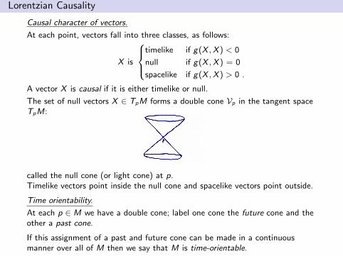
The set of null vectors X ∈ TpM forms a double cone Vp in the tangent spaceTpM:

called the null cone (or light cone) at p.Timelike vectors point inside the null cone and spacelike vectors point outside.

Time orientability.

At each p ∈ M we have a double cone; label one cone the future cone and theother a past cone.

If this assignment of a past and future cone can be made in a continuousmanner over all of M then we say that M is time-orientable.


Time orientability (cont.).

There are various ways to make the phrase “continuous assignment” precise(see e.g., O’Neill p. 145), but they all result in the following:

Fact: A Lorentzian manifold Mn+1 is time-orientable iff it admits a smoothtimelike vector field T .

If M is time-orientable, the choice of a smooth time-like vector field T fixes atime orientation on M: A causal vector X ∈ TpM is future pointing if it pointsinto the same half-cone as T , and past pointing otherwise.

(Remark: If M is not time-orientable, it admits a double cover that is.)

By a spacetime we mean a connected time-oriented Lorentzian manifold(Mn+1, g).


Causal character of curves.

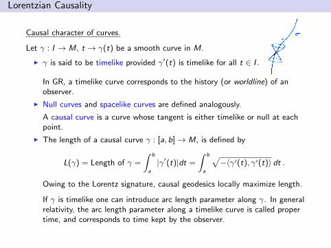
Let γ : I → M, t → γ(t) be a smooth curve in M.

I γ is said to be timelike provided γ′(t) is timelike for all t ∈ I .

In GR, a timelike curve corresponds to the history (or worldline) of anobserver.

I Null curves and spacelike curves are defined analogously.

A causal curve is a curve whose tangent is either timelike or null at eachpoint.

I The length of a causal curve γ : [a, b]→ M, is defined by

L(γ) = Length of γ =

∫ b

a

|γ′(t)|dt =

∫ b

a

√−〈γ′(t), γ′(t)〉 dt .

Owing to the Lorentz signature, causal geodesics locally maximize length.

If γ is timelike one can introduce arc length parameter along γ. In generalrelativity, the arc length parameter along a timelike curve is called propertime, and corresponds to time kept by the observer.


Futures and Pasts

Let (M, g) be a spacetime. A timelike (resp. causal) curve γ : I → M is said tobe future directed provided each tangent vector γ′(t), t ∈ I , is future pointing.(Past-directed timelike and causal curves are defined in a time-dual manner.)

Causal theory is the study of the causal relations and <:

Definition 1.1

For p, q ∈ M,

1. p q means there exists a future directed timelike curve in M from p toq (we say that q is in the timelike future of p),

2. p < q means there exists a (nontrivial) future directed causal curve in Mfrom p to q (we say that q is in the causal future of p),

We shall use the notation p ≤ q to mean p = q or p < q.

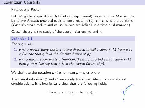
The causal relations and < are clearly transitive. Also, from variationalconsiderations, it is heuristically clear that the following holds,

if p q and q < r then p r .


Proposition 1.1 (O’Neill, p. 294)

In a spacetime M, if q is in the causal future of p (p < q) but is not in thetimelike future of p (p 6 q) then any future directed causal curve γ from p toq must be a null geodesic (when suitably parameterized).

Now introduce standard causal notation:

Definition 1.2

Given any point p in a spacetime M, the timelike future and causal future of p,denoted I +(p) and J+(p), respectively, are defined as,

I +(p) = q ∈ M : p q and J+(p) = q ∈ M : p ≤ q .

The timelike and causal pasts of p, I−(p) and J−(p), respectively, are definedin a time-dual manner in terms of past directed timelike and causal curves.

With respect to this notation, the above proposition becomes:

Propostion If q ∈ J+(p) \ I +(p) (q 6= p) then there exists a future directednull geodesic from p to q.


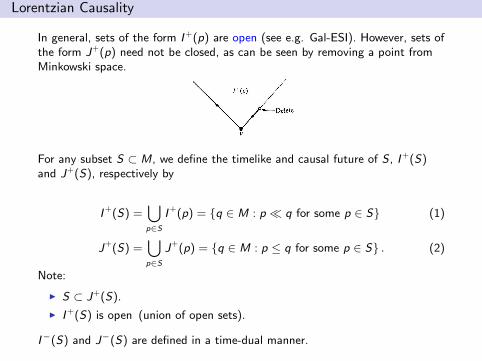
In general, sets of the form I +(p) are open (see e.g. Gal-ESI). However, sets ofthe form J+(p) need not be closed, as can be seen by removing a point fromMinkowski space.

For any subset S ⊂ M, we define the timelike and causal future of S , I +(S)and J+(S), respectively by

I +(S) =⋃p∈S

I +(p) = q ∈ M : p q for some p ∈ S (1)

J+(S) =⋃p∈S

J+(p) = q ∈ M : p ≤ q for some p ∈ S . (2)

Note:

I S ⊂ J+(S).

I I +(S) is open (union of open sets).

I−(S) and J−(S) are defined in a time-dual manner.


Achronal Boundaries

Achronal sets play an important role in causal theory.

Definition 1.3

A subset S ⊂ M is achronal provided no two of its points can be joined by atimelike curve.

Of particular importance are achronal boundaries.

Definition 1.4

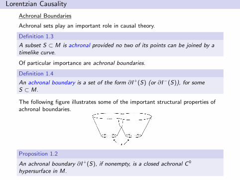
An achronal boundary is a set of the form ∂I +(S) (or ∂I−(S)), for someS ⊂ M.

The following figure illustrates some of the important structural properties ofachronal boundaries.

Proposition 1.2

An achronal boundary ∂I +(S), if nonempty, is a closed achronal C 0

hypersurface in M.


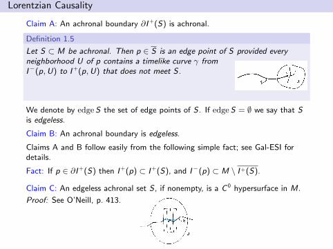
Claim A: An achronal boundary ∂I +(S) is achronal.

Definition 1.5

Let S ⊂ M be achronal. Then p ∈ S is an edge point of S provided everyneighborhood U of p contains a timelike curve γ fromI−(p,U) to I +(p,U) that does not meet S.

We denote by edgeS the set of edge points of S . If edgeS = ∅ we say that Sis edgeless.

Claim B: An achronal boundary is edgeless.

Claims A and B follow easily from the following simple fact; see Gal-ESI fordetails.

Fact: If p ∈ ∂I +(S) then I +(p) ⊂ I +(S), and I−(p) ⊂ M \ I +(S).

Claim C: An edgeless achronal set S , if nonempty, is a C 0 hypersurface in M.

Proof: See O’Neill, p. 413.

Monday, September 7, 15


Causality conditions

A number of results in Lorentzian geometry and general relativity require somesort of causality condition.

Chronology condition: A spacetime M satisfies the chronology conditionprovided there are no closed timelike curves in M.

Compact spacetimes have limited interest in general relativity since they allviolate the chronology condition.

Proposition 1.3

Every compact spacetime contains a closed timelike curve.

Proof: The sets I +(p); p ∈ M form an open cover of M from which we canabstract a finite subcover: I +(p1), I +(p2), ..., I +(pk ). We may assume thatthis is the minimal number of such sets covering M. Since these sets cover M,p1 ∈ I +(pi ) for some i . It follows that I +(p1) ⊂ I +(pi ). Hence, if i 6= 1, wecould reduce the number of sets in the cover. Thus, p1 ∈ I +(p1) which impliesthat there is a closed timelike curve through p1.

A somewhat stronger condition than the chronology condition is the

Causality condition: A spacetime M satisfies the causality condition providedthere are no closed (nontrivial) causal curves in M.


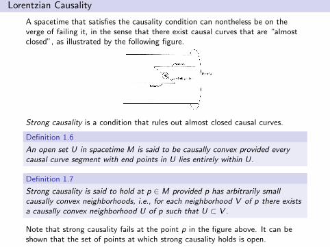
A spacetime that satisfies the causality condition can nontheless be on theverge of failing it, in the sense that there exist causal curves that are “almostclosed”, as illustrated by the following figure.

Strong causality is a condition that rules out almost closed causal curves.

Definition 1.6

An open set U in spacetime M is said to be causally convex provided everycausal curve segment with end points in U lies entirely within U.

Definition 1.7

Strong causality is said to hold at p ∈ M provided p has arbitrarily smallcausally convex neighborhoods, i.e., for each neighborhood V of p there existsa causally convex neighborhood U of p such that U ⊂ V .

Note that strong causality fails at the point p in the figure above. It can beshown that the set of points at which strong causality holds is open.


Strong causality condition: A spacetime M is said to be strongly causal ifstrong causality holds at all of its points.

This is the “standard” causality condition in spacetime geometry, and, althoughthere are even stronger causality conditions, it is sufficient for most applications.

The following lemma is often useful.

Lemma 1.4

Suppose strong causality holds at each point of a compact set K in aspacetime M. If γ : [0, b)→ M is a future inextendible causal curve that startsin K then eventually it leaves K and does not return, i.e., there existst0 ∈ [0, b) such that γ(t) /∈ K for all t ∈ [t0, b).

(γ is future inextendible if it cannot be continuously extended, i.e. iflimt→b− γ(t) does not exist.)

We say that a future inextendible causal curve cannot be “imprisoned” in acompact set on which strong causality holds.


Global hyperbolicity

We now come to a fundamental condition in spacetime geometry, that ofglobal hyperbolicity.

Mathematically, global hyperbolicity is a basic ‘niceness’ condition that oftenplays a role analogous to geodesic completeness in Riemannian geometry.Physically, global hyperbolicity is closely connected to the issue of classicaldeterminism and the strong cosmic censorship conjecture.

Definition 1.8

A spacetime M is said to be globally hyperbolic provided

I M is strongly causal.

I (Internal Compactness) The sets J+(p) ∩ J−(q) are compact for allp, q ∈ M.

Remarks:

1. Condition (2) says roughly that M has no holes or gaps.

2. In fact, as shown by Bernal and Sanchez [4], internal compactness +causality imply strong causality.


Proposition 1.5

Let M be a globally hyperbolic spacetime. Then,

1. The sets J±(A) are closed, for all compact A ⊂ M.

2. The sets J+(A) ∩ J−(B) are compact, for all compact A,B ⊂ M.

Global hyperbolicity is the standard condition in Lorentzian geometry thatensures the existence of maximal causal geodesic segments.

Theorem 1.6

Let M be a globally hyperbolic spacetime. If q ∈ J+(p) then there is a maximalfuture directed causal geodesic from p to q (i.e., no causal curve from p to qcan have greater length).

See Gal-ESI for discussions of the proofs.

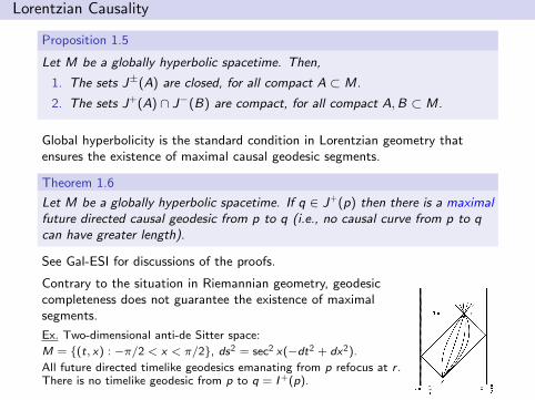
Contrary to the situation in Riemannian geometry, geodesiccompleteness does not guarantee the existence of maximalsegments.

Ex. Two-dimensional anti-de Sitter space:

M = (t, x) : −π/2 < x < π/2, ds2 = sec2 x(−dt2 + dx2).

All future directed timelike geodesics emanating from p refocus at r .There is no timelike geodesic from p to q = I +(p).


Cauchy hypersurfaces

Global hyperbolicity is closely related to the existence of certain ‘ideal initialvalue hypersurfaces’, called Cauchy surfaces. There are slight variations in theliterature in the definition of a Cauchy surface. Here we adopt the followingdefinition.

Definition 1.9

A Cauchy surface for a spacetime M is an achronal subset S of M which is metby every inextendible causal curve in M.

Observations:

I If S is a Cauchy surface for M then ∂I +(S) = S . (Also ∂I−(S) = S .) Itfollows from Proposition 1.2 that a Cauchy surface S is a closed achronalC 0 hypersurface in M.

I If S is Cauchy then every inextendible timelike curve meets S exactly once.

Theorem 1.7 (Geroch)

If a spacetime M is globally hyperbolic then it has a Cauchy surface S.

We make some comments about the proof. (As discussed later, the conversealso holds.)


I Introduce a measure µ on M such that µ(M) = 1, and consider thefunctionf : M → R defined by

f (p) =µ(J−(p))

µ(J+(p)).

I Internal compactness is used to show that f is continuous, and strongcausality is used to show that f is strictly increasing along future directedcausal curves.

I Moreover, if γ : (a, b)→ M is a future directed inextendible causal curvein M, one shows f (γ(t))→ 0 as t → a+, and f (γ(t))→∞ as t → b−.

I It follows that ‘slices’ of f , e.g., S = p ∈ M : f (p) = 1, are Cauchysurfaces for M.

Remark: The function f constructed in the proof is what is referred to as atime function, namely, a continuous function that is strictly increasing alongfuture directed causal curves.

Bernal and Sanchez [3] have shown how to construct smooth time functions,i.e., smooth functions with (past directed) timelike gradient, which hence arenecessarily time functions. (See also Chrusciel, Grant and Minguzzi [6] forrelated developments.)


Proposition 1.8

Let M be globally hyperbolic.

I If S is a Cauchy surface for M then M is homeomorphic to R× S.

I Any two Cauchy surfaces in M are homeomorphic.

Proof: To prove the first, one introduces a future directed timelike vector fieldX on M. Each integral curve of X meets S exactly once. These integralcurves, suitably parameterized, provide the desired homeomorphism. A similartechnique may be used to prove the second.

Remark: In view of Proposition 1.8, any nontrivial topology in a globallyhyperbolic spacetime must reside in its Cauchy surfaces.

The following fact is often useful.

Proposition 1.9

If S is a compact achronal C 0 hypersurface in a globally hyperbolic spacetimeM then S must be a Cauchy surface for M.


Proposition 1.9

If S is a compact achronal C 0 hypersurface in a globally hyperbolic spacetimeM then S must be a Cauchy surface for M.

Comments on the proof:

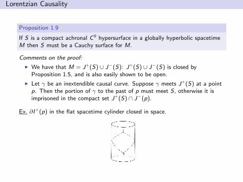
I We have that M = J+(S) ∪ J−(S): J+(S) ∪ J−(S) is closed byProposition 1.5, and is also easily shown to be open.

I Let γ be an inextendible causal curve. Suppose γ meets J+(S) at a pointp. Then the portion of γ to the past of p must meet S , otherwise it isimprisoned in the compact set J+(S) ∩ J−(p).

Ex. ∂I +(p) in the flat spacetime cylinder closed in space.


Domains of Dependence

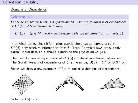
Definition 1.10

Let S be an achronal set in a spacetime M. The future domain of dependenceof D+(S) of S is defined as follows,

D+(S) = p ∈ M : every past inextendible causal curve from p meets S

In physical terms, since information travels along causal curves, a point inD+(S) only receives information from S . Thus if physical laws are suitablycausal, initial data on S should determine the physics on D+(S).

The past domain of dependence of D−(S) is defined in a time-dual manner.The (total) domain of dependence of S is the union, D(S) = D+(S) ∪ D−(S).

Below we show a few examples of future and past domains of dependence.

Note: D+(S) ⊃ S .


The following characterizes Cauchy surfaces in terms of domain of dependence.

Proposition 1.10

Let S be an achronal subset of a spacetime M. Then, S is a Cauchy surface for M ifand only if D(S) = M.

Proof: Exercise.

The following basic result ties domains of dependence to global hyperbolicity.

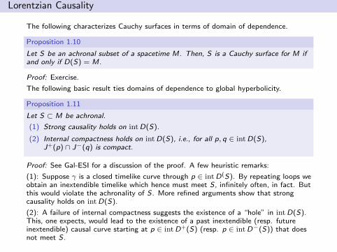
Proposition 1.11

Let S ⊂ M be achronal.

(1) Strong causality holds on intD(S).

(2) Internal compactness holds on intD(S), i.e., for all p, q ∈ intD(S),J+(p) ∩ J−(q) is compact.

Proof: See Gal-ESI for a discussion of the proof. A few heuristic remarks:

(1): Suppose γ is a closed timelike curve through p ∈ intD(S). By repeating loops weobtain an inextendible timelike which hence must meet S, infinitely often, in fact. Butthis would violate the achronality of S. More refined arguments show that strongcausality holds on intD(S).

(2): A failure of internal compactness suggests the existence of a “hole” in intD(S).This, one expects, would lead to the existence of a past inextendible (resp. futureinextendible) causal curve starting at p ∈ intD+(S) (resp. p ∈ intD−(S)) that doesnot meet S .


By Proposition 1.11, for S ⊂ M achronal, intD(S) is globally hyperbolic.

Hence, we can now address the converse of Theorem 1.7.

Corollary 1.12

If S is a Cauchy surface for M then M is globally hyperbolic.

Proof: This follows immediately from Propositions 1.10 and 1.11: S Cauchy=⇒ D(S) = M =⇒ intD(S) = M =⇒ M is globally hyperbolic.

Thus we have that: M is globally hyperbolic if and only if M admits a Cauchysurface.


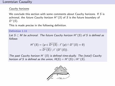
Cauchy horizons

We conclude this section with some comments about Cauchy horizons. If S isachronal, the future Cauchy horizon H+(S) of S is the future boundary ofD+(S).

This is made precise in the following definition.

Definition 1.11

Let S ⊂ M be achronal. The future Cauchy horizon H+(S) of S is defined asfollows

H+(S) = p ∈ D+(S) : I +(p) ∩ D+(S) = ∅

= D+(S) \ I−(D+(S)) .

The past Cauchy horizon H−(S) is defined time-dually. The (total) Cauchyhorizon of S is defined as the union, H(S) = H+(S) ∪ H−(S).


We record some basic facts about domains of dependence and Cauchy horizons.

Proposition 1.13

Let S be an achronal subset of M. Then the following hold.

1. H+(S) is achronal.

2. ∂D+(S) = H+(S) ∪ S.

3. ∂D(S) = H(S).

Point 3 provides a useful mechanism for showing that an achronal set S isCauchy: S is Cauchy iff D(S) = M iff ∂D(S) = ∅ iff H(S) = ∅.

Cauchy horizons have structural properties similar to achronal boundaries, asindicated in the next two results.

Proposition 1.14

Let S ⊂ M be achronal. Then H+(S) \ edgeH+(S), if nonempty, is anachronal C 0 hypersurface in M.

Proposition 1.15

Let S be an achronal subset of M. Then H+(S) is ruled by null geodesics, i.e.,every point of H+(S)\ edgeS is the future endpoint of a null geodesic in H+(S)which is either past inextendible in M or else has a past end point on edgeS.

The geometry of null hypersurfaces

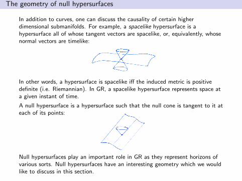
In addition to curves, one can discuss the causality of certain higherdimensional submanifolds. For example, a spacelike hypersurface is ahypersurface all of whose tangent vectors are spacelike, or, equivalently, whosenormal vectors are timelike:

In other words, a hypersurface is spacelike iff the induced metric is positivedefinite (i.e. Riemannian). In GR, a spacelike hypersurface represents space ata given instant of time.

A null hypersurface is a hypersurface such that the null cone is tangent to it ateach of its points:

Null hypersurfaces play an important role in GR as they represent horizons ofvarious sorts. Null hypersurfaces have an interesting geometry which we wouldlike to discuss in this section.


Comments on Curvature and the Einstein Equations

I Let ∇ : X(M)× X(M)→ X(M), (X ,Y )→ ∇X Y , be the Levi-Civitaconnection with respect to the Lorentz metric g . ∇ is determined locallyby the Christoffel symbols,

∇∂i ∂j =∑

k

Γkij ∂k , (∂i =

∂

∂x i, etc.)

I Geodesics are curves t → σ(t) of zero acceleration,

∇σ′(t)σ′(t) = 0 .

Timelike geodesics correspond to free falling observers.I The Riemann curvature tensor is defined by,

R(X ,Y )Z = ∇X∇Y Z −∇Y∇X Z −∇[X ,Y ]Z

The components R`kij are determined by,

R(∂i , ∂j )∂k =∑`

R`kij∂`

I The Ricci tensor Ric and scalar curvature R are obtained by taking traces,

Rij =∑`

R`i`j and R =

∑i,j

g ij Rij


I The Einstein equations, the field equations of GR, are given by:

Rij −1

2Rgij = 8πTij ,

where Tij is the energy-momentum tensor.

I From the PDE point of view, the Einstein equations form a system ofsecond order quasi-linear equations for the gij ’s. This system may beviewed as a (highly complicated!) generalization of Poisson’s equation inNewtonian gravity.

I The vacuum Einstein equations are obtained by setting Tij = 0. It is easilyseen that this equivalent to setting Rij = 0.

We will sometimes require that a spacetime satisfying the Einsteinequations, obeys an energy condition.

I The null energy condition (NEC) is the requirement that

T (X ,X ) =∑

i,j

Tij Xi X j ≥ 0 for all null vectors X .

I The stronger dominant energy condtion (DEC) is the requirement,

T (X ,Y ) =∑

i,j

Tij Xi Y j ≥ 0 for all future directed causal vectors X ,Y .


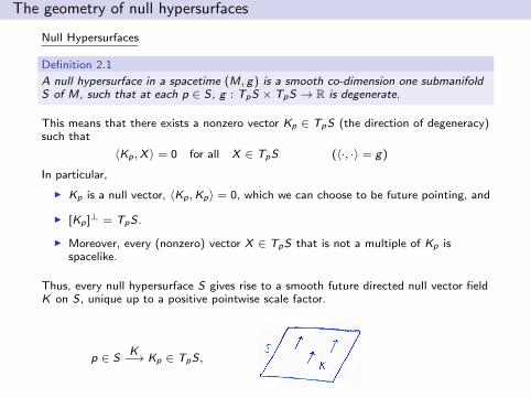
Null Hypersurfaces

Definition 2.1

A null hypersurface in a spacetime (M, g) is a smooth co-dimension one submanifoldS of M, such that at each p ∈ S, g : TpS × TpS → R is degenerate.

This means that there exists a nonzero vector Kp ∈ TpS (the direction of degeneracy)such that

〈Kp ,X 〉 = 0 for all X ∈ TpS (〈·, ·〉 = g)

In particular,

I Kp is a null vector, 〈Kp ,Kp〉 = 0, which we can choose to be future pointing, and

I [Kp ]⊥ = TpS .

I Moreover, every (nonzero) vector X ∈ TpS that is not a multiple of Kp isspacelike.

Thus, every null hypersurface S gives rise to a smooth future directed null vector fieldK on S, unique up to a positive pointwise scale factor.

p ∈ SK−→ Kp ∈ TpS,


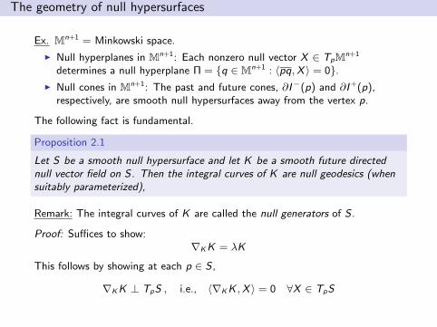
Ex. Mn+1 = Minkowski space.

I Null hyperplanes in Mn+1: Each nonzero null vector X ∈ TpMn+1

determines a null hyperplane Π = q ∈ Mn+1 : 〈pq,X 〉 = 0.I Null cones in Mn+1: The past and future cones, ∂I−(p) and ∂I +(p),

respectively, are smooth null hypersurfaces away from the vertex p.

The following fact is fundamental.

Proposition 2.1

Let S be a smooth null hypersurface and let K be a smooth future directednull vector field on S. Then the integral curves of K are null geodesics (whensuitably parameterized),

Remark: The integral curves of K are called the null generators of S .

Proof: Suffices to show:∇K K = λK

This follows by showing at each p ∈ S ,

∇K K ⊥ TpS , i.e., 〈∇K K ,X 〉 = 0 ∀X ∈ TpS


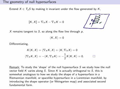
Extend X ∈ TpS by making it invariant under the flow generated by K ,

[K ,X ] = ∇K X −∇X K = 0

X remains tangent to S , so along the flow line through p,

〈K ,X 〉 = 0

Differentiating,

K〈K ,X 〉 = 〈∇K K ,X 〉+ 〈K ,∇K X 〉 = 0

〈∇K K ,X 〉 = −〈K ,∇X K〉 = −1

2X 〈K ,K〉 = 0.

Remark: To study the ‘shape’ of the null hypersurface S we study how the nullvector field K varies along S . Since K is actually orthogonal to S , this issomewhat analogous to how we study the shape of a hypersurface in aRiemannian manifold, or spacelike hypersurface in a Lorentzian manifold, byintroducing the shape operator (or Weingarten map) and associated secondfundamental form.


Null Weingarten Map/Null 2nd Fundamental Form

I We introduce the following equivalence relation on tangent vectors: ForX ,Y ∈ TpS ,

X = Y mod K ⇐⇒ X − Y = λK

Let X denote the equivalence class of X ∈ TpS and let,

TpS/K = X : X ∈ TpS

Then,

TS/K = ∪p∈S TpS/K

is a rank n− 1 vector bundle over S (n = dimS). This vector bundle doesnot depend on the particular choice of null vector field K .

I There is a natural positive definite metric h on TS/K induced from 〈 , 〉:For each p ∈ S , define h : TpS/K × TpS/K → R by

h(X ,Y ) = 〈X ,Y 〉.

Well-defined: If X ′ = X mod K , Y ′ = Y mod K then

〈X ′,Y ′〉 = 〈X + αK ,Y + βK〉= 〈X ,Y 〉+ β〈X ,K〉+ α〈K ,Y 〉+ αβ〈K ,K〉= 〈X ,Y 〉 .


I The null Weingarten map b = bK of S with respect to K is, for each pointp ∈ S , a linear map b : TpS/K → TpS/K defined by

b(X ) = ∇X K .

b is well-defined: X ′ = X mod K ⇒

∇X ′K = ∇X +αK K

= ∇X K + α∇K K = ∇X K + αλK

= ∇X K mod K

I b is self adjoint with respect to h, i.e., h(b(X ),Y ) = h(X , b(Y )), for allX ,Y ∈ TpS/K .

Proof: Extend X ,Y ∈ TpS to vector fields tangent to S near p. UsingX 〈K ,Y 〉 = 0 and Y 〈K ,X 〉 = 0, we obtain,

h(b(X ),Y ) = h(∇X K ,Y ) = 〈∇X K ,Y 〉= −〈K ,∇X Y 〉 = −〈K ,∇Y X 〉+ 〈K , [X ,Y ]〉

= 〈∇Y K ,X 〉 = h(X , b(Y )) .


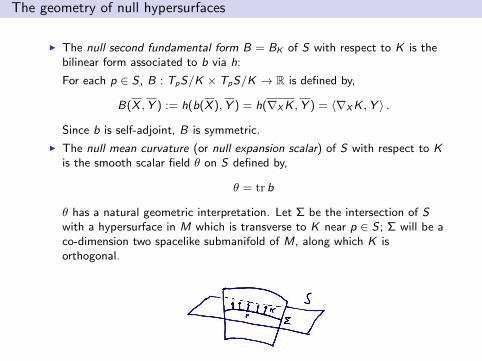
I The null second fundamental form B = BK of S with respect to K is thebilinear form associated to b via h:

For each p ∈ S , B : TpS/K × TpS/K → R is defined by,

B(X ,Y ) := h(b(X ),Y ) = h(∇X K ,Y ) = 〈∇X K ,Y 〉 .

Since b is self-adjoint, B is symmetric.

I The null mean curvature (or null expansion scalar) of S with respect to Kis the smooth scalar field θ on S defined by,

θ = tr b

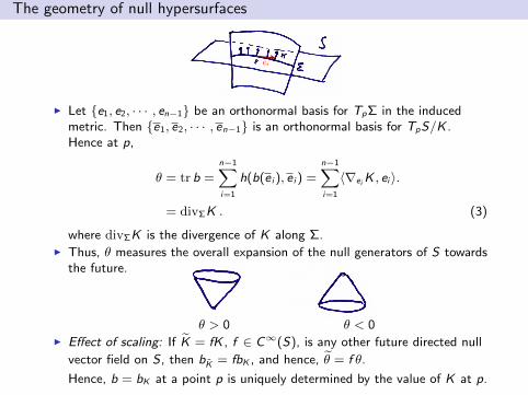
θ has a natural geometric interpretation. Let Σ be the intersection of Swith a hypersurface in M which is transverse to K near p ∈ S ; Σ will be aco-dimension two spacelike submanifold of M, along which K isorthogonal.


ei

I Let e1, e2, · · · , en−1 be an orthonormal basis for TpΣ in the inducedmetric. Then e1, e2, · · · , en−1 is an orthonormal basis for TpS/K .Hence at p,

θ = tr b =n−1∑i=1

h(b(e i ), e i ) =n−1∑i=1

〈∇ei K , ei 〉.

= divΣK . (3)

where divΣK is the divergence of K along Σ.I Thus, θ measures the overall expansion of the null generators of S towards

the future.

θ > 0 θ < 0I Effect of scaling: If K = fK , f ∈ C∞(S), is any other future directed null

vector field on S , then bK = fbK , and hence, θ = f θ.

Hence, b = bK at a point p is uniquely determined by the value of K at p.


Comparison Theory

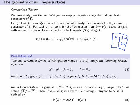
We now study how the null Weingarten map propagates along the null geodesicgenerators of S .

Let η : I → M, s → η(s), be a future directed affinely parameterized null geodesicgenerator of S . For each s ∈ I , consider the Weingarten map b = b(s) based at η(s)with respect to the null vector field K which equals η′(s) at η(s),

b(s) = bη′(s) : Tη(s)S/η′(s)→ Tη(s)S/η′(s)

Proposition 2.2

The one parameter family of Weingarten maps s → b(s), obeys the following Riccatiequation,

b′ + b2 + R = 0 , ′ = ∇η′ (4)

where R : Tη(s)S/η′(s)→ Tη(s)S/η′(s) is given by R(X ) = R(X , η′(s))η′(s).

Remark on notation: In general, if Y = Y (s) is a vector field along η tangent to S , we

define, (Y )′ = Y ′. Then, if X = X (s) is a vector field along η tangent to S, b′ isdefined by,

b′(X ) := b(X )′ − b(X ′) . (5)


Proof: Fix a point p = η(s0), s0 ∈ (a, b), on η. On a neighborhood U of p in Swe can scale the null vector field K so that K is a geodesic vector field,∇K K = 0, and so that K , restricted to η, is the velocity vector field to η, i.e.,for each s near s0, Kη(s) = η′(s). Let X ∈ TpM. Shrinking U if necessary, wecan extend X to a smooth vector field on U so that[X ,K ] = ∇X K −∇K X = 0. Then,

R(X ,K)K = ∇X∇K K −∇K∇X K −∇[X ,K ]K = −∇K∇K X

Hence along η we have,

X ′′ = −R(X , η′)η′

(which implies that X , restricted to η, is a Jacobi field along η).

Thus, from Equation (5), at the point p we have,

b′(X ) = ∇X K ′ − b(∇K X ) = ∇K X ′ − b(∇X K)

= X ′′ − b(b(X )) = −R(X , η′)η′ − b2(X )

= −R(X )− b2(X ),

which establishes Equation (4).


By taking the trace of (4) we obtain the following formula for the derivative ofthe null mean curvature θ = θ(s) along η,

θ′ = −Ric(η′, η′)− σ2 − 1

n − 1θ2, (6)

where σ := (tr b2)1/2 is the shear scalar, b := b − 1n−1

θ · id is the trace free

part of the Weingarten map, and Ric(η′, η′) is the spacetime Ricci tensorevaluated on the tangent vector η′.

Equation 6 is known in relativity as the Raychaudhuri equation (for anirrotational null geodesic congruence). This equation shows how the Riccicurvature of spacetime influences the null mean curvature of a nullhypersurface.

We consider a basic application of the Raychaudhuri equation.

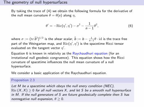
Proposition 2.3

Let M be a spacetime which obeys the null enery condition (NEC),Ric (X ,X ) ≥ 0 for all null vectors X , and let S be a smooth null hypersurfacein M. If the null generators of S are future geodesically complete then S hasnonnegative null expansion, θ ≥ 0.


Proof: Suppose θ < 0 at p ∈ S . Let s → η(s) be the null generator of Spassing through p = η(0), affinely parametrized. Let b(s) = bη′(s), and takeθ = tr b. By the invariance of sign under scaling, one has θ(0) < 0.

Raychaudhuri’s equation and the NEC imply that θ = θ(s) obeys the inequality,

dθ

ds≤ − 1

n − 1θ2 ,

and hence θ < 0 for all s > 0. Dividing through by θ2 then gives,

d

ds

(1

θ

)≥ 1

n − 1,

which implies 1/θ → 0, i.e., θ → −∞ in finite affine parameter time,contradicting the smoothness of θ.

Remark. Let Σ be a local cross section of the null hypersurface S (see earlierfigure) with volume form ω. If Σ is moved under flow generated by K thenLKω = θ ω, where L = Lie derivative.

Thus, Proposition 2.3 implies, under the given assumptions, that cross sectionsof S are nondecreasing in area as one moves towards the future. Proposition2.3 is the simplest form of Hawking’s black hole area theorem [16]. For a studyof the area theorem, with a focus on issues of regularity, see [6].

The Penrose singularity theorem and related results

In this section we introduce the important notion of a trapped surface andpresent the classical Penrose singularity theorem.

I Let (Mn+1, g) be an (n + 1)-dimensional spacetime, n ≥ 3.

Let Σn−1 be a closed (i.e., compact without boundary) co-dimension twospacelike submanifold of M.

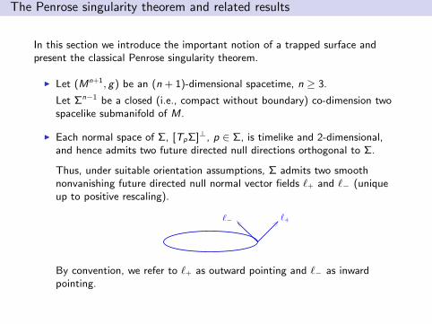
I Each normal space of Σ, [TpΣ]⊥, p ∈ Σ, is timelike and 2-dimensional,and hence admits two future directed null directions orthogonal to Σ.

Thus, under suitable orientation assumptions, Σ admits two smoothnonvanishing future directed null normal vector fields `+ and `− (uniqueup to positive rescaling).

MATHEMATICAL GENERAL RELATIVITY 61

and if its generators are future complete then Proposition 7.1 implies that E hasnonnegative null expansion. This in turn implies that “cross-sections” of E arenondecreasing in area as one moves towards the future, as asserted by the areatheorem. In the context of black hole thermodynamics, the area theorem is referredto as the second law of black mechanics, and provides a link between gravity andquantum physics. As it turns out, the area theorem remains valid without imposingany smoothness assumptions; for a recent study of the area theorem, which focuseson these issues of regularity, see [131].

7.2. Trapped and marginally trapped surfaces. We begin with some defini-tions. Let ! = !n!1, n ! 3, be a spacelike submanifold of co-dimension two in aspace-time (M n+1, g). Regardless of the dimension of space-time, we shall refer to! as a surface, which it actually is in the 3 + 1 case. We are primarily interestedin the case where ! is compact (without boundary), and so we simply assume thisfrom the outset.

Each normal space of !, [Tp!]", p " !, is timelike and 2-dimensional, andhence admits two future directed null directions orthogonal to !. Thus, if thenormal bundle is trivial, ! admits two smooth nonvanishing future directed nullnormal vector fields l+ and l!, which are unique up to positive pointwise scaling,see Figure 7.1. By convention, we refer to l+ as outward pointing and l! as inwardpointing.21 In relativity it is standard to decompose the second fundamental form

l# l+

Figure 7.1. The null future normals l± to !.

of ! into two scalar valued null second forms !+ and !!, associated to l+ and l!,respectively. For each p " !, !± : Tp! $ Tp! % R is the bilinear form defined by,

!±(X, Y ) = g(&X l±, Y ) for all X, Y " Tp! .(7.5)

A standard argument shows that !± is symmetric. Hence, !+ and !! can be tracedwith respect to the induced metric " on ! to obtain the null mean curvatures (ornull expansion scalars),

(7.6) #± = tr! !± = "ij(!±)ij = div!l± .

#± depends on the scaling of l± in a simple way. As follows from Equation (7.5),multiplying l± by a positive function f simply scales #± by the same function.Thus, the sign of #± does not depend on the scaling of l±. Physically, #+ (resp.,#!) measures the divergence of the outgoing (resp., ingoing) light rays emanatingfrom !.

It is useful to note the connection between the null expansion scalars #± and theexpansion of the generators of a null hypersurface, as discussed in Section 7.1. LetN+ be the null hypersurface, defined and smooth near !, generated by the null

21In many situations, there is a natural choice of “inward” and “outward”.

`+`

By convention, we refer to `+ as outward pointing and `− as inwardpointing.


I Associated to `+ and `−, are the two null second fundamental forms, χ+

and χ−, respectively, defined as

χ± : TpΣ× TpΣ→ R, χ±(X ,Y ) = g(∇X `±,Y ) .

I The null expansion scalars (or null mean curvatures) θ± of Σ are obtainedby tracing χ± with respect to the induced metric γ on Σ,

θ± = trγχ± = γABχ±AB = div Σ`± .

The sign of θ± does not depend on the scaling of `±. Physically, θ+

(resp., θ−) measures the divergence of the outgoing (resp., ingoing) lightrays emanating orthogonally from Σ.

Remark: There is a natural connection between these null expansionscalars θ± and the null expansion of null hypersurfaces: `+ locallygenerates a smooth null hypersurface S+. Then θ+ is the null expansion ofS+ restricted to Σ; θ− may be described similarly.


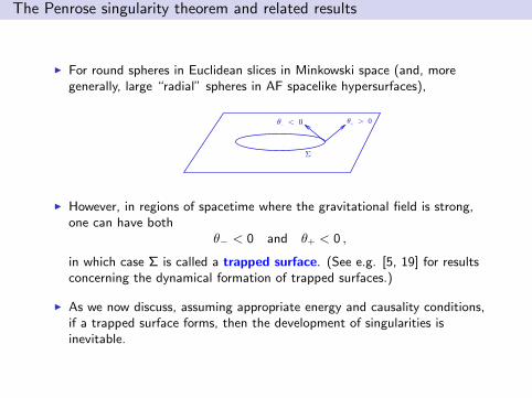
I For round spheres in Euclidean slices in Minkowski space (and, moregenerally, large “radial” spheres in AF spacelike hypersurfaces),

§

0> +µ 0< µ

I However, in regions of spacetime where the gravitational field is strong,one can have both

θ− < 0 and θ+ < 0 ,

in which case Σ is called a trapped surface. (See e.g. [5, 19] for resultsconcerning the dynamical formation of trapped surfaces.)

I As we now discuss, assuming appropriate energy and causality conditions,if a trapped surface forms, then the development of singularities isinevitable.


Theorem 3.1 (Penrose singularity theorem)

Let M be a globally hyperbolic spacetime which satisfies the NEC,Ric(X ,X ) ≥ 0 for all null vectors X , and which has a noncompact Cauchysurface S. If M contains a trapped surface Σ then M is future null geodesicallyincomplete.

Proof: We first observe the following.

Claim: ∂I +(Σ) is noncompact.

Proof of Claim: ∂I +(Σ) is an achronal boundary, and hence, byProposition 1.2, is an achronal C 0 hypersurface. If ∂I +(Σ) were compact then,by Proposition 1.9, ∂I +(Σ) would be a compact Cauchy surface. But thiswould contradict the assumption that S is noncompact (all Cauchy surfaces arehomeomorphic).

We now construct a future inextendible null geodesic in ∂I +(Σ), which weshow must be future incomplete.


I We have that

∂I +(S) = I +(S) \ int I +(S) = J+(S) \ I +(S) .

It then follows from Proposition 1.1 that each q ∈ ∂I +(Σ) lies on a nullgeodesic in ∂I +(Σ) with past end point on Σ. Moreover this null geodesicmeets Σ orthogonally (due to achronality, cf. O’Neill [22, Lemma 50, p.298]).

I Since ∂I +(Σ) is closed and noncompact, there exists a sequence of pointsqk ⊂ ∂I +(Σ) that diverges to infinity. For each k, there is a nullgeodesic ηk from Σ to qk , which is contained in ∂I +(Σ) and meets Σorthogonally.

I By compactness of Σ, some subsequence ηkj converges to a futureinextendible null geodesic η contained in ∂I +(Σ), and meeting Σorthogonally (at p, say).

η must be future incomplete. Suppose not.


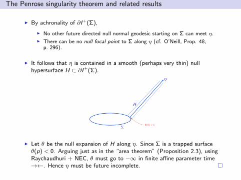
I By achronality of ∂I +(Σ),

I No other future directed null normal geodesic starting on Σ can meet η.

I There can be no null focal point to Σ along η (cf. O’Neill, Prop. 48,p. 296).

I It follows that η is contained in a smooth (perhaps very thin) nullhypersurface H ⊂ ∂I +(Σ).

(0) < 0

H

I Let θ be the null expansion of H along η. Since Σ is a trapped surfaceθ(p) < 0. Arguing just as in the “area theorem” (Proposition 2.3), usingRaychaudhuri + NEC, θ must go to −∞ in finite affine parameter time→←. Hence η must be future incomplete.

Topics

1 Lorentzian Causality

2 The Geometry of Null Hypersurfaces

3 The Penrose Singularity Theorem and Related Results

4 Marginally Outer Trapped Surfaces and the Topology of Black Holes

5 The Geometry and Topology of the Exterior Region


For certain applications, the following variant of the Penrose singularitytheorem is useful.

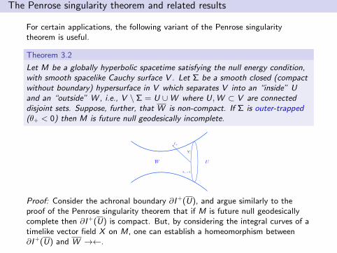
Theorem 3.2

Let M be a globally hyperbolic spacetime satisfying the null energy condition,with smooth spacelike Cauchy surface V . Let Σ be a smooth closed (compactwithout boundary) hypersurface in V which separates V into an “inside” Uand an “outside” W , i.e., V \ Σ = U ∪W where U,W ⊂ V are connecteddisjoint sets. Suppose, further, that W is non-compact. If Σ is outer-trapped(θ+ < 0) then M is future null geodesically incomplete.

W U

`+

+ < 0

Proof: Consider the achronal boundary ∂I +(U), and argue similarly to theproof of the Penrose singularity theorem that if M is future null geodesicallycomplete then ∂I +(U) is compact. But, by considering the integral curves of atimelike vector field X on M, one can establish a homeomorphism between∂I +(U) and W →←.


This version of the Penrose singularity theorem may be used to prove thefollowing beautiful result of Gannon [15] and Lee [20].

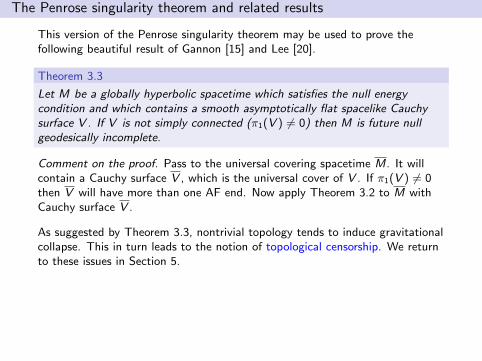
Theorem 3.3

Let M be a globally hyperbolic spacetime which satisfies the null energycondition and which contains a smooth asymptotically flat spacelike Cauchysurface V . If V is not simply connected (π1(V ) 6= 0) then M is future nullgeodesically incomplete.

Comment on the proof. Pass to the universal covering spacetime M. It willcontain a Cauchy surface V , which is the universal cover of V . If π1(V ) 6= 0then V will have more than one AF end. Now apply Theorem 3.2 to M withCauchy surface V .

As suggested by Theorem 3.3, nontrivial topology tends to induce gravitationalcollapse. This in turn leads to the notion of topological censorship. We returnto these issues in Section 5.

Marginally outer trapped surfaces and the topology of black holes

Introduction

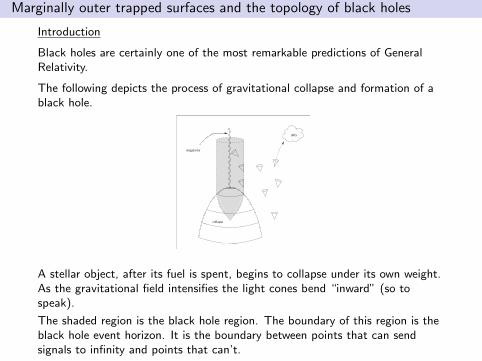
Black holes are certainly one of the most remarkable predictions of GeneralRelativity.

The following depicts the process of gravitational collapse and formation of ablack hole.

singularity

collapse

infty

A stellar object, after its fuel is spent, begins to collapse under its own weight.As the gravitational field intensifies the light cones bend “inward” (so tospeak).

The shaded region is the black hole region. The boundary of this region is theblack hole event horizon. It is the boundary between points that can sendsignals to infinity and points that can’t.


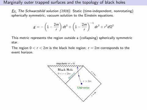
Ex. The Schwarzshild solution (1916). Static (time-independent, nonrotating)spherically symmetric, vacuum solution to the Einstein equations.

g = −(

1− 2m

r

)dt2 +

(1− 2m

r

)−1

dr 2 + r 2dΩ2

This metric represents the region outside a (collapsing) spherically symmetricstar.

The region 0 < r < 2m is the black hole region; r = 2m corresponds to theevent horizon.

r > 2m

0 < r < 2m


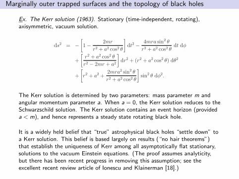
Ex. The Kerr solution (1963). Stationary (time-independent, rotating),axisymmetric, vacuum solution.

The Kerr spacetime: A brief introduction Matt Visser 14

Here the second line is again simply flat 3-space in disguise. An advantageof this coordinate system is that t can naturally be thought of as a timecoordinate — at least at large distances near spatial infinity. There arehowever still 3 off-diagonal terms in the metric so this is not yet any greatadvance on the original form (3). One can easily consider the limits m → 0,a → 0, and the decomposition of this metric into Kerr–Schild form, but thereare no real surprises.

Second, it is now extremely useful to perform a further m-dependent coor-dinate transformation, which will put the line element into Boyer–Lindquistform:

t = tBL + 2m

∫r dr

r2 − 2mr + a2; φ = −φBL − a

∫dr

r2 − 2mr + a2; (55)

r = rBL; θ = θBL. (56)

Making the transformation, and dropping the BL subscript, the Kerr line-element now takes the form:

ds2 = −[1 − 2mr

r2 + a2 cos2 θ

]dt2 − 4mra sin2 θ

r2 + a2 cos2 θdt dφ (57)

+

[r2 + a2 cos2 θ

r2 − 2mr + a2

]dr2 + (r2 + a2 cos2 θ) dθ2

+

[r2 + a2 +

2mra2 sin2 θ

r2 + a2 cos2 θ

]sin2 θ dφ2.

• These Boyer–Lindquist coordinates are particularly useful in that theyminimize the number of off-diagonal components of the metric — thereis now only one off-diagonal component. We shall subsequently seethat this helps particularly in analyzing the asymptotic behaviour, andin trying to understand the key difference between an “event horizon”and an “ergosphere”.

• Another particularly useful feature is that the asymptotic (r → ∞)behaviour in Boyer–Lindquist coordinates is

ds2 = −[1 − 2m

r+ O

(1

r3

)]dt2 −

[4ma sin2 θ

r+ O

(1

r3

)]dφ dt

+

[1 +

2m

r+ O

(1

r2

)] [dr2 + r2(dθ2 + sin2 θ dφ2)

]. (58)

The Kerr solution is determined by two parameters: mass parameter m andangular momentum parameter a. When a = 0, the Kerr solution reduces to theSchwarzschild solution. The Kerr solution contains an event horizon (provideda < m), and hence represents a steady state rotating black hole.

It is a widely held belief that “true” astrophysical black holes “settle down” toa Kerr solution. This belief is based largely on results (“no hair theorems”)that establish the uniqueness of Kerr among all asymptotically flat stationary,solutions to the vacuum Einstein equations. (The proof assumes analyticity,but there has been recent progress in removing this assumption; see theexcellent recent review article of Ionescu and Klainerman [18].)


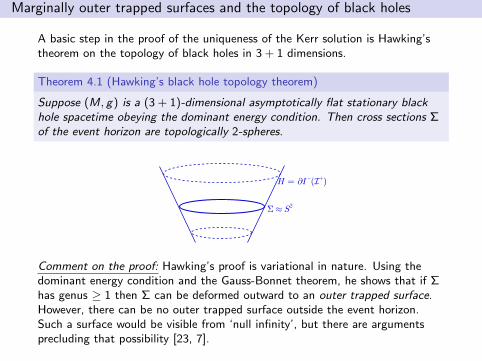
A basic step in the proof of the uniqueness of the Kerr solution is Hawking’stheorem on the topology of black holes in 3 + 1 dimensions.

Theorem 4.1 (Hawking’s black hole topology theorem)

Suppose (M, g) is a (3 + 1)-dimensional asymptotically flat stationary blackhole spacetime obeying the dominant energy condition. Then cross sections Σof the event horizon are topologically 2-spheres.

2S¼§

)+I(@I = H

Comment on the proof: Hawking’s proof is variational in nature. Using thedominant energy condition and the Gauss-Bonnet theorem, he shows that if Σhas genus ≥ 1 then Σ can be deformed outward to an outer trapped surface.However, there can be no outer trapped surface outside the event horizon.Such a surface would be visible from ‘null infinity’, but there are argumentsprecluding that possibility [23, 7].


Higher Dimensional Black Holes

I String theory, and various related developments (e.g., the AdS/CFTcorrespondence, braneworld scenarios, entropy calculations) havegenerated a great deal of interest in gravity in higher dimensions, and inparticular, in higher dimensional black holes.

I One of the first questions to arise was:

Does black hole uniqueness hold in higher dimensions?

I With impetus coming from the development of string theory, in 1986,Myers and Perry [21] constructed natural higher dimensionalgeneralizations of the Kerr solution. These models painted a pictureconsistent with the situation in 3 + 1 dimensions. In particular, they havespherical horizon topology.


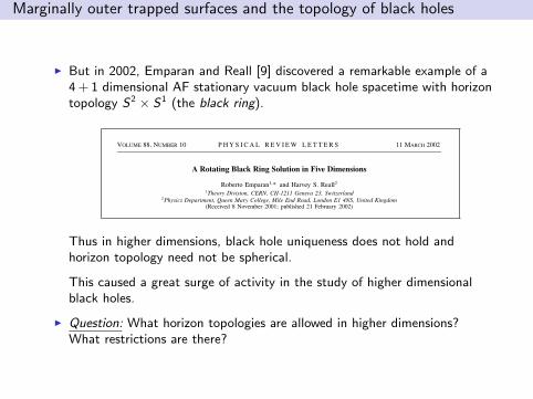
I But in 2002, Emparan and Reall [9] discovered a remarkable example of a4 + 1 dimensional AF stationary vacuum black hole spacetime with horizontopology S2 × S1 (the black ring).

VOLUME 88, NUMBER 10 P H Y S I C A L R E V I E W L E T T E R S 11 MARCH 2002

A Rotating Black Ring Solution in Five Dimensions

Roberto Emparan1,* and Harvey S. Reall21Theory Division, CERN, CH-1211 Geneva 23, Switzerland

2Physics Department, Queen Mary College, Mile End Road, London E1 4NS, United Kingdom(Received 8 November 2001; published 21 February 2002)

The vacuum Einstein equations in five dimensions are shown to admit a solution describing a stationaryasymptotically flat spacetime regular on and outside an event horizon of topology S1 3 S2. It describesa rotating “black ring.” This is the first example of a stationary asymptotically flat vacuum solution withan event horizon of nonspherical topology. The existence of this solution implies that the uniquenesstheorems valid in four dimensions do not have simple five-dimensional generalizations. It is suggestedthat increasing the spin of a spherical black hole beyond a critical value results in a transition to a blackring, which can have an arbitrarily large angular momentum for a given mass.

DOI: 10.1103/PhysRevLett.88.101101 PACS numbers: 04.50.+h, 04.20.Jb, 04.70.Bw

Black holes in four spacetime dimensions are highlyconstrained objects. A number of classical theorems showthat a stationary, asymptotically flat, vacuum black holeis completely characterized by its mass and spin [1], andevent horizons of nonspherical topology are forbidden [2].

In this Letter we show explicitly that in five dimen-sions the situation cannot be so simple by exhibiting anasymptotically flat, stationary, vacuum solution with ahorizon of topology S1 3 S2: a black ring. The ringrotates along the S1 and this balances its gravitationalself-attraction. The solution is characterized by its massM and spin J. The black hole of [3] with rotation ina single plane (and horizon of topology S3) can be ob-tained as a branch of the same family of solutions. Weshow that there exist black holes and black rings withthe same values of M and J. They can be distinguished

by their topology and by their mass dipole measuredat infinity. This shows that there is no obvious five-dimensional analog of the uniqueness theorems.

S1 3 S2 is one of the few possible topologies for theevent horizon in five dimensions that was not ruled out bythe analysis in [4] (although this argument does not applydirectly to our black ring because it assumes time symme-try). An explicit solution with a regular (but degenerate)horizon of topology S1 3 S2 and spacelike infinity withS3 topology has been built recently in [5]. An unchargedstatic black ring solution is presented in [6], but it containsconical singularities. Our solution is the first asymptot-ically flat vacuum solution that is completely regular onand outside an event horizon of nonspherical topology.

Our starting point is the following metric, constructedas a Wick-rotated version of a solution in [7]:

ds2 2FxFy

µdt 1

rn

j1

j2 2 y

Adc

∂2

11

A2x 2 y2

∑2Fx

µG ydc2 1

F yG y

dy2∂

1 F y2µ

dx2

Gx1

GxFx

df2∂∏

, (1)

where j2 is defined below and

Fj 1 2 jj1, Gj 1 2 j2 1 nj3. (2)

The solution of [7] was obtained as the electric dual ofthe magnetically charged Kaluza-Klein C metric of [8].Our metric can be related directly to the latter solution byanalytic continuation. When n 0 we recover the staticblack ring solution of [6].

We assume that 0 , n , n 23p

3, which en-sures that the roots of Gj are all distinct and real. Theywill be ordered as j2 , j3 , j4. It is easy to establishthat 21 , j2 , 0 , 1 , j3 , j4 ,

1n . A double root

j3 j4 appears when n n. Without loss of generality,we take A . 0. Taking A , 0 simply reverses the senseof rotation.

We take x to lie in the range j2 # x # j3 and requirethat j1 $ j3, which ensures that gxx , gff $ 0. In order

to avoid a conical singularity at x j2 we identify f withperiod

Df 4p

pFj2

G0j2

4pp

j1 2 j2

np

j1 j3 2 j2 j4 2 j2.

(3)

A metric of Lorentzian signature is obtained by takingy , j2. Examining the behavior of the constant t slices of(1), one finds that c must be identified with period Dc Df in order to avoid a conical singularity at y j2 fi x.Regularity of the full metric here can be demonstrated byconverting from the polar coordinates y, c to Cartesiancoordinates — the dtdc term can then be seen to vanishsmoothly at the origin y j2.

There are now two cases of interest depending on thevalue of j1. One of these will correspond to a black ring

101101-1 0031-90070288(10)101101(4)$20.00 © 2002 The American Physical Society 101101-1

Thus in higher dimensions, black hole uniqueness does not hold andhorizon topology need not be spherical.

This caused a great surge of activity in the study of higher dimensionalblack holes.

I Question: What horizon topologies are allowed in higher dimensions?What restrictions are there?


Marginally Outer Trapped Surfaces

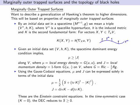
Want to describe a generalization of Hawking’s theorem to higher dimensions.This will be based on properties of marginally outer trapped surfaces.

I By an initial data set in a spacetime (Mn+1, g) we mean a triple(V n, h,K), where V n is a spacelike hypersurface, h is the induced metricand K is the second fundamental form: For vectors X ,Y ∈ TpV ,

K(X ,Y ) = h(∇X u,Y )

I Given an initial data set (V , h,K), the spacetime dominant energycondition implies,

µ ≥ |J|along V , where µ = local energy density = G(u, u), and J = localmomentum density = 1-form G(u, ·) on V , where G = Ric − 1

2Rg .

I Using the Gauss-Codazzi equations, µ and J can be expressed solely interms of the initial data

µ =1

2

(S + (trK)2 − |K |2

),

J = divK − d(trK) .

These are the Einstein constraint equations. In the time-symmetric case(K = 0), the DEC reduces to S ≥ 0.


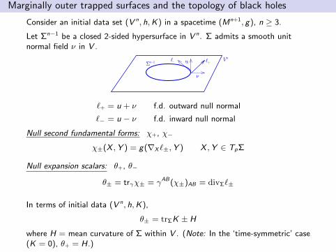
Consider an initial data set (V n, h,K) in a spacetime (Mn+1, g), n ≥ 3.

Let Σn−1 be a closed 2-sided hypersurface in V n. Σ admits a smooth unitnormal field ν in V .

+``1n§nVu

º

`+ = u + ν f.d. outward null normal

`− = u − ν f.d. inward null normal

Null second fundamental forms: χ+, χ−

χ±(X ,Y ) = g(∇X `±,Y ) X ,Y ∈ TpΣ

Null expansion scalars: θ+, θ−

θ± = trγχ± = γAB (χ±)AB = divΣ`±

In terms of initial data (V n, h,K),

θ± = trΣK ± H

where H = mean curvature of Σ within V . (Note: In the ‘time-symmetric’ case(K = 0), θ+ = H.)


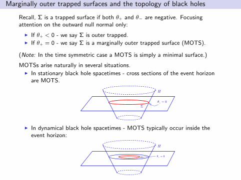
Recall, Σ is a trapped surface if both θ+ and θ− are negative. Focusingattention on the outward null normal only:

I If θ+ < 0 - we say Σ is outer trapped.I If θ+ = 0 - we say Σ is a marginally outer trapped surface (MOTS).

(Note: In the time symmetric case a MOTS is simply a minimal surface.)

MOTSs arise naturally in several situations.I In stationary black hole spacetimes - cross sections of the event horizon

are MOTS.

= 0+µ

§

H

I In dynamical black hole spacetimes - MOTS typically occur inside theevent horizon:

= 0+µ

H


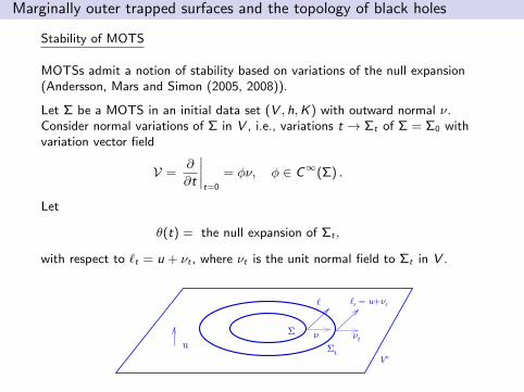
Stability of MOTS

MOTSs admit a notion of stability based on variations of the null expansion(Andersson, Mars and Simon (2005, 2008)).

Let Σ be a MOTS in an initial data set (V , h,K) with outward normal ν.Consider normal variations of Σ in V , i.e., variations t → Σt of Σ = Σ0 withvariation vector field

V =∂

∂t

∣∣∣∣t=0

= φν, φ ∈ C∞(Σ) .

Let

θ(t) = the null expansion of Σt ,

with respect to `t = u + νt , where νt is the unit normal field to Σt in V .

tºu

t§

§

nV

tº+u = t``

º


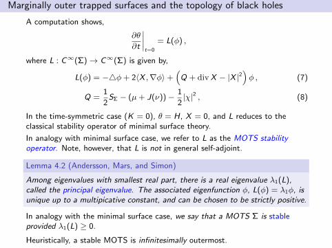
A computation shows,

∂θ

∂t

∣∣∣∣t=0

= L(φ) ,

where L : C∞(Σ)→ C∞(Σ) is given by,

L(φ) = −4φ+ 2〈X ,∇φ〉+(

Q + divX − |X |2)φ , (7)

Q =1

2SΣ − (µ+ J(ν))− 1

2|χ|2 , (8)

In the time-symmetric case (K = 0), θ = H, X = 0, and L reduces to theclassical stability operator of minimal surface theory.

In analogy with minimal surface case, we refer to L as the MOTS stabilityoperator. Note, however, that L is not in general self-adjoint.

Lemma 4.2 (Andersson, Mars, and Simon)

Among eigenvalues with smallest real part, there is a real eigenvalue λ1(L),called the principal eigenvalue. The associated eigenfunction φ, L(φ) = λ1φ, isunique up to a multipicative constant, and can be chosen to be strictly positive.

In analogy with the minimal surface case, we say that a MOTS Σ is stableprovided λ1(L) ≥ 0.

Heuristically, a stable MOTS is infinitesimally outermost.


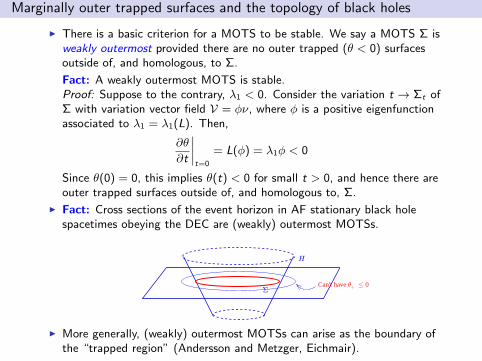
I There is a basic criterion for a MOTS to be stable. We say a MOTS Σ isweakly outermost provided there are no outer trapped (θ < 0) surfacesoutside of, and homologous, to Σ.

Fact: A weakly outermost MOTS is stable.Proof: Suppose to the contrary, λ1 < 0. Consider the variation t → Σt ofΣ with variation vector field V = φν, where φ is a positive eigenfunctionassociated to λ1 = λ1(L). Then,

∂θ

∂t

∣∣∣∣t=0

= L(φ) = λ1φ < 0

Since θ(0) = 0, this implies θ(t) < 0 for small t > 0, and hence there areouter trapped surfaces outside of, and homologous to, Σ.

I Fact: Cross sections of the event horizon in AF stationary black holespacetimes obeying the DEC are (weakly) outermost MOTSs.

0· +µCan't have

H

§

I More generally, (weakly) outermost MOTSs can arise as the boundary ofthe “trapped region” (Andersson and Metzger, Eichmair).


A Generalization of Hawking’s Black Hole Topology Theorem

Theorem 4.3 (G. and Schoen [14])

Let (V , h,K) be an n-dimensional initial data set, n ≥ 3, satisfying thedominant energy condition (DEC), µ ≥ |J|. If Σ is a stable MOTS in V then(apart from certain exceptional circumstances) Σ must be of positive Yamabetype, i.e. must admit a metric of positive scalar curvature.

Remarks.

I The theorem may be viewed as a spacetime analogue of a fundamentalresult of Schoen and Yau concerning stable minimal hypersurfaces inmanifolds of positive scalar curvature.

I The ‘exceptional circumstances’ are ruled out if, for example, the DECholds strictly at some point of Σ or Σ is not Ricci flat.

I Σ being of positive Yamabe type implies many well-known restrictions onthe topology (see e.g.; see e.g. [17, Chapter 7]).

We consider here two basic examples, and for simplicity we assume Σ isorientable.


Case 1. dim Σ = 2 (dim M = 3 + 1): In this case, Σ being of positive Yamabetype means that Σ admits a metric of positive Gaussian curvature. Hence, bythe Gauss-Bonnet theorem, Σ is topologically a 2-sphere, and we recoverHawking’s theorem.

Case 2. dim Σ = 3 (dim M = 4 + 1).

Theorem. (Gromov-Lawson, Schoen-Yau) If Σ is a closed orientable3-manifold of positive Yamabe type then Σ must be diffeomorphic to:

I a spherical space, or

I S2 × S1, or

I a connected sum of the above two types.

Remark: By the prime decomposition theorem, Σ must be a connected sum of(1) spherical spaces, (2) S2 × S1’s, and (3) K(π, 1) manifolds. But since Σ ispositive Yamabe, it cannot contain any K(π, 1)’s in its prime decomposition.

Thus, the basic horizon topologies in dim Σ = 3 case are S3 and S2 × S1.

(Kundari and Lucietti have recently constructed an AF black hole spacetimesatisfying the DEC with RP3 horizon topology, arXiv 2014.)


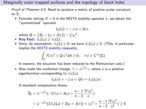
Proof of Theorem 4.3: Need to produce a metric of positive scalar curvatureon Σ.

I Formally setting X = 0 in the MOTS stability operator L, we obtain the”symmetrized” operator

L0(φ) = −4φ+ Q φ .

where Q = 12SΣ − (µ+ J(ν))− 1

2|χ|2.

I Key Fact: λ1(L0) ≥ λ1(L).I Since, by assumption, λ1(L) ≥ 0, we have λ1(L0) ≥ 0. (This, in particular,

implies the MOTS stability inequality,∫Σ

|∇ψ|2 + Q ψ2dA ≥ 0 , ∀ψ ∈ C∞(Σ)

In essence, the situation has been reduced to the Riemannian case.)

I Now make the conformal change: γ = φ2

n−2 γ, where φ is a positiveeigenfunction corresponding to λ1(L0):

L0(φ) = −4φ+ Qφ = λ1(L0)φ .

A standard computation shows,

SΣ = φ−n

n−2 (−24φ+ SΣφ+n − 1

n − 2

|∇φ|2

φ)

= φ−2

n−2 (2λ1(L0) + 2(µ+ J(ν)) + |χ|2 +n − 1

n − 2

|∇φ|2

φ2) ≥ 0


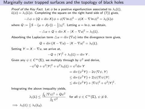
Proof of the Key Fact. Let φ be a positive eigenfunction associated to λ1(L),L(φ) = λ1(L)φ. Completing the square on the right hand side of (7)) gives,

−4φ+ (Q + div X )φ+ φ|∇ lnφ|2 − φ|X −∇ lnφ|2 = λ1(L)φ

where Q := 12

S − (µ+ J(ν))− 12|χ|2. Letting u = lnφ, we obtain,

−4u + Q + div X − |X −∇u|2 = λ1(L) .

Absorbing the Laplacian term 4u = div (∇u) into the divergence term gives,

Q + div (X −∇u)− |X −∇u|2 = λ1(L).

Setting Y = X −∇u, we arrive at,

−Q + |Y |2 + λ1(L) = div Y .

Given any ψ ∈ C∞(Σ), we multiply through by ψ2 and derive,

−ψ2Q + ψ2|Y |2 + ψ2λ1(L) = ψ2div Y

= div (ψ2Y )− 2ψ〈∇ψ,Y 〉

≤ div (ψ2Y ) + 2|ψ||∇ψ||Y |

≤ div (ψ2Y ) + |∇ψ|2 + ψ2|Y |2 .

Integrating the above inequality yields,

λ1(L) ≤∫

Σ |∇ψ|2 + Qψ2∫

Σ ψ2

for all ψ ∈ C∞(Σ), ψ 6≡ 0 .

=⇒ λ1(L) ≤ λ1(L0).


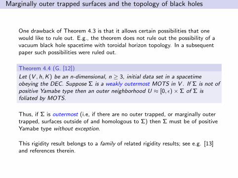
One drawback of Theorem 4.3 is that it allows certain possibilities that onewould like to rule out. E.g., the theorem does not rule out the possibility of avacuum black hole spacetime with toroidal horizon topology. In a subsequentpaper such possibilities were ruled out.

Theorem 4.4 (G. [12])

Let (V , h,K) be an n-dimensional, n ≥ 3, initial data set in a spacetimeobeying the DEC. Suppose Σ is a weakly outermost MOTS in V . If Σ is not ofpositive Yamabe type then an outer neighborhood U ≈ [0, ε)× Σ of Σ isfoliated by MOTS.

Thus, if Σ is outermost (i.e, if there are no outer trapped, or marginally outertrapped, surfaces outside of and homologous to Σ) then Σ must be of positiveYamabe type without exception.

This rigidity result belongs to a family of related rigidity results; see e.g. [13]and references therein.

Topics

1 Lorentzian Causality

2 The Geometry of Null Hypersurfaces

3 The Penrose Singularity Theorem and Related Results

4 Marginally Outer Trapped Surfaces and the Topology of Black Holes

5 The Geometry and Topology of the Exterior Region

The geometry and topology of the exterior region

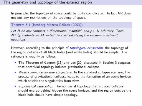
In principle, the topology of space could be quite complicated. In fact GR doesnot put any restrictions on the topology of space.

Theorem 5.1 (Isenberg-Mazzeo-Pollack (2003))

Let N be any compact n-dimensional manifold, and p ∈ N arbitrary. ThenN \ p admits an AF initial data set satisfying the vacuum constraintequations.

However, according to the principle of topological censorship, the topology ofthe region outside of all black holes (and white holes) should be simple. Therationale is roughly as follows:

I The Theorem of Gannon [15] and Lee [20] discussed in Section 3 suggeststhat nontrivial topology induces gravitational collapse.

I Weak cosmic censorship conjecture: In the standard collapse scenario, theprocess of gravitational collapse leads to the formation of an event horizonwhich shields the singularities from view.

I Topological censorship: The nontrivial topology that induced collapseshould end up behind hidden the event horizon, and the region outside theblack hole should have simple topology.


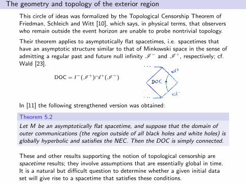
This circle of ideas was formalized by the Topological Censorship Theorem ofFriedman, Schleich and Witt [10], which says, in physical terms, that observerswho remain outside the event horizon are unable to probe nontrivial topology.

Their theorem applies to asymptotically flat spacetimes, i.e. spacetimes thathave an asymptotic structure similar to that of Minkowski space in the sense ofadmitting a regular past and future null infinity I− and I +, respectively; cf.Wald [23].

DOC = I−(I +)∩I +(I−)

In [11] the following strengthened version was obtained:

Theorem 5.2

Let M be an asymptotically flat spacetime, and suppose that the domain ofouter communications (the region outside of all black holes and white holes) isglobally hyperbolic and satisfies the NEC. Then the DOC is simply connected.

These and other results supporting the notion of topological censorship arespacetime results; they involve assumptions that are essentially global in time.It is a natural but difficult question to determine whether a given initial dataset will give rise to a spacetime that satisfies these conditions.


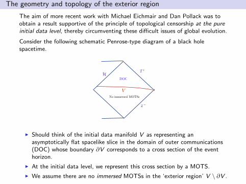
The aim of more recent work with Michael Eichmair and Dan Pollack was toobtain a result supportive of the principle of topological censorship at the pureinitial data level, thereby circumventing these difficult issues of global evolution.

Consider the following schematic Penrose-type diagram of a black holespacetime.

I+

I

H

VNo immersed MOTSs

DOC

I Should think of the initial data manifold V as representing anasymptotically flat spacelike slice in the domain of outer communications(DOC) whose boundary ∂V corresponds to a cross section of the eventhorizon.

I At the initial data level, we represent this cross section by a MOTS.

I We assume there are no immersed MOTSs in the ‘exterior region’ V \ ∂V .


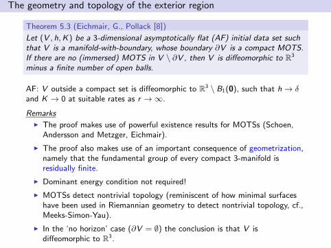
Theorem 5.3 (Eichmair, G., Pollack [8])

Let (V , h,K) be a 3-dimensional asymptotically flat (AF) initial data set suchthat V is a manifold-with-boundary, whose boundary ∂V is a compact MOTS.If there are no (immersed) MOTS in V \ ∂V , then V is diffeomorphic to R3

minus a finite number of open balls.

AF: V outside a compact set is diffeomorphic to R3 \ B1(0), such that h→ δand K → 0 at suitable rates as r →∞.

Remarks

I The proof makes use of powerful existence results for MOTSs (Schoen,Andersson and Metzger, Eichmair).

I The proof also makes use of an important consequence of geometrization,namely that the fundamental group of every compact 3-manifold isresidually finite.

I Dominant energy condition not required!

I MOTSs detect nontrivial topology (reminiscent of how minimal surfaceshave been used in Riemannian geometry to detect nontrivial topology, cf.,Meeks-Simon-Yau).

I In the ‘no horizon’ case (∂V = ∅) the conclusion is that V isdiffeomorphic to R3.


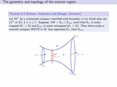
Theorem 5.4 (Schoen, Andersson and Metzger, Eichmair)

Let W n be a connected compact manifold-with-boundary in an initial data set(V n, h,K), 3 ≤ n ≤ 7. Suppose, ∂W = Σin ∪ Σout , such that Σin is outertrapped (θ+ < 0) and Σout is outer untrapped (θ+ > 0). Then there exists asmooth compact MOTS in W that separates Σin from Σout .

!"#!

$

!

%

"#&"$' "#("$')"%"#$'

!in


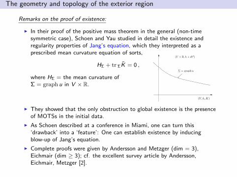
Remarks on the proof of existence:

I In their proof of the positive mass theorem in the general (non-timesymmetric case), Schoen and Yau studied in detail the existence andregularity properties of Jang’s equation, which they interpreted as aprescribed mean curvature equation of sorts,

HΣ + tr ΣK = 0 ,

where HΣ = the mean curvature ofΣ = graph u in V × R.

JANG’S EQUATION AND MARGINAL SURFACES 3

(M, g, k)

(M, g, k)

(M × R, g + dt2)

Figure 2.

Assuming that the triple (M, g, k) is the induced geometric data for a hypersurfacein a spacetime satisfying the dominant energy condition, the induced scalar cur-vature is non-negative modulo a divergence term (which of course can be large).Jang then, following the approach taken by Geroch in the case of non-negativescalar curvature, introduces a modified inverse mean curvature flow depending ona solution of Jang’s equation, as well as an adapted Geroch mass that he shows tobe formally monotone along his flow. If these steps outlined by Jang can be maderigorous, then his arguments lead to a proof of the positive energy theorem in thisgeneral situation.

Jang’s work has not been developed further due to the fact that an effectivetheory for existence and regularity of solutions of Jang’s equation (4) was lackinguntil the work of Schoen and Yau, who applied Jang’s equation differently from theoriginal intention by using it to reduce the space-time positive mass theorem to thetime symmetric case. Further, it is not clear how to define an appropriate weaksolution of the modified IMCF introduced by Jang.

1.1. Jang’s equation and positivity of mass. A complete proof of the positivemass theorem was first given by Schoen and Yau [51], for the special case of time-symmetric initial data. They then extended their result to general, asympoticallyflat initial data satisfying the dominant energy condition by using Jang’s equationto “improve” the properties of the initial data in [55]. We describe here severalaspects of Jang’s equation which play a fundamental role in their work.

Firstly, Jang’s equation is closely analogous to the equation

(5) HΣ + trΣ(k) = 0

defining marginally outer trapped surfaces Σ ⊂ M , where as above HΣ, trΣ(k) arethe mean curvature of Σ and the trace of k restricted to Σ, respectively.

Equations of minimal surface type may have blow-up solutions on general do-mains and an important step in [55] is the analysis of the blow-up sets for thesolutions of Jang’s equation. At the boundaries of the blow-up sets, the graph of uis asymptotically vertical, asymptotic to cylinders over marginally outer (or inner)trapped surfaces – here the above mentioned relation of Jang’s equation to theMOTS equation comes into play.

Secondly, the induced geometry of the graph M of a solution of Jang’s equationcan be confomally changed to a metric with zero scalar curvature without increasingthe mass.

The fundamental reason for this is that the analogue of the stability operator forM , i.e., the linearization of Jang’s equation, has, in a certain sense, non-negative

(V R, h + dt2)

(V, h, K)

= graph u

I They showed that the only obstruction to global existence is the presenceof MOTSs in the initial data.

I As Schoen described at a conference in Miami, one can turn this‘drawback’ into a ‘feature’: One can establish existence by inducingblow-up of Jang’s equation.

I Complete proofs were given by Andersson and Metzger (dim = 3),Eichmair (dim ≥ 3); cf. the excellent survey article by Andersson,Eichmair, Metzger [2].


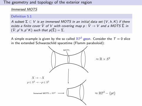
Immersed MOTS

Definition 5.1

A subset Σ ⊂ V is an immersed MOTS in an initial data set (V , h,K) if thereexists a finite cover V of V with covering map p : V → V and a MOTS Σ in(V , p∗h, p∗K) such that p(Σ) = Σ.

A simple example is given by the so called RP3 geon. Consider the T = 0 slicein the extended Schwarzschild spacetime (Flamm paraboloid):

p 2 S2 ! p 2 S2

R S2

RP3 ptImmersed MOTS = RP2

MOTS

X ! X


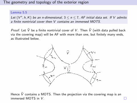
Lemma 5.5

Let (V n, h,K) be an n-dimensional, 3 ≤ n ≤ 7, AF initial data set. If V admitsa finite nontrivial cover then V contains an immersed MOTS.

Proof: Let V be a finite nontrivial cover of V . Then V (with data pulled backvia the covering map) will be AF with more than one, but finitely many ends,as illustrated below.

Hence V contains a MOTS. Then the projection via the covering map is animmersed MOTS in V .


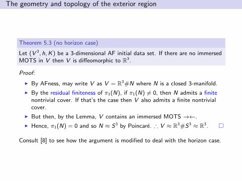
Theorem 5.3 (no horizon case)

Let (V 3, h,K) be a 3-dimensional AF initial data set. If there are no immersedMOTS in V then V is diffeomorphic to R3.

Proof:

I By AFness, may write V as V = R3#N where N is a closed 3-manifold.

I By the residual finiteness of π1(N), if π1(N) 6= 0, then N admits a finitenontrivial cover. If that’s the case then V also admits a finite nontrivialcover.

I But then, by the Lemma, V contains an immersed MOTS →←.

I Hence, π1(N) = 0 and so N ≈ S3 by Poincare. ∴ V ≈ R3#S3 ≈ R3.

Consult [8] to see how the argument is modified to deal with the horizon case.


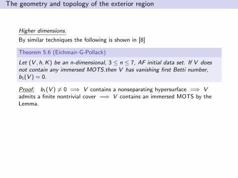
Higher dimensions.

By similar techniques the following is shown in [8]

Theorem 5.6 (Eichmair-G-Pollack)

Let (V , h,K) be an n-dimensional, 3 ≤ n ≤ 7, AF initial data set. If V doesnot contain any immersed MOTS.then V has vanishing first Betti number,b1(V ) = 0.

Proof: b1(V ) 6= 0 =⇒ V contains a nonseparating hypersurface =⇒ Vadmits a finite nontrivial cover =⇒ V contains an immersed MOTS by theLemma.


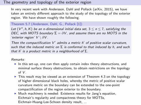
In very recent work with Andersson, Dahl and Pollack (arXiv, 2015), we havetaken an entirely different approach to the study of the topology of the exteriorregion. We have shown roughly the following.

Theorem 5.7 (Andersson, Dahl, G., Pollack [1])

Let (V n, h,K) be an n-dimensional initial data set, 3 ≤ n ≤ 7, satisfying theDEC, with MOTS boundary Σ = ∂V , and assume there are no MOTS in the‘exterior region’ V \ ∂V .

Then the compactification V ′ admits a metric h′ of positive scalar curvature,such that the induced metric on Σ is conformal to that induced by h, and suchthat h′ is a product metric in a neighborhood of Σ.

Remarks:I In this set-up, one can then apply certain index theory obstructions, and

minimal surface theory obstructions, to obtain restrictions on the topologyof V .

I This result may be viewed as an extension of Theorem 4.3 on the topologyof higher dimensional black holes, whereby the metric of positive scalarcurvature metric on the boundary can be extended to the one-pointcompactification of the region exterior to the boundary.

I Much machinery is needed: Existence results for Jang’s equation,Eichmair’s regularity and compactness theory for MOTSs,Eichmair-Huang-Lee-Schoen density result, ...

References

[1] L. Andersson, M. Dahl, G. J. Galloway, and D. Pollack, On the geometry andtopology of initial data sets with horizons, 2015, arXiv:1508.01896.

[2] L. Andersson, M. Eichmair, and J. Metzger, Jang’s equation and its applicationsto marginally trapped surfaces, Complex analysis and dynamical systems IV. Part2, Contemp. Math., vol. 554, Amer. Math. Soc., Providence, RI, 2011, pp. 13–45.

[3] A. N. Bernal and M. Sanchez, Smoothness of time functions and the metricsplitting of globally hyperbolic spacetimes, Comm. Math. Phys. 257 (2005),no. 1, 43–50.

[4] , Globally hyperbolic spacetimes can be defined as ‘causal’ instead of‘strongly causal’, Classical Quantum Gravity 24 (2007), no. 3, 745–749.

[5] D. Christodoulou, The formation of black holes in general relativity, Geometryand analysis. No. 1, Adv. Lect. Math. (ALM), vol. 17, Int. Press, Somerville, MA,2011, pp. 247–283.

[6] P. T. Chrusciel, E. Delay, G. J. Galloway, and R. Howard, Regularity of horizonsand the area theorem, Ann. Henri Poincare 2 (2001), no. 1, 109–178.

[7] P. T. Chrusciel, G. J. Galloway, and D. Solis, Topological censorship forKaluza-Klein space-times, Ann. Henri Poincare 10 (2009), no. 5, 893–912.

[8] M. Eichmair, G. J. Galloway, and D. Pollack, Topological censorship from theinitial data point of view, J. Differential Geom. 95 (2013), no. 3, 389–405.

[9] R. Emparan and H. S. Reall, A rotating black ring solution in five dimensions,Phys. Rev. Lett. 88 (2002), no. 10, 101101, 4.

[10] J. L. Friedman, K. Schleich, and D. M. Witt, Topological censorship, Phys. Rev.Lett. 71 (1993), no. 10, 1486–1489.

[11] G. J. Galloway, On the topology of the domain of outer communication, ClassicalQuantum Gravity 12 (1995), no. 10, L99–L101.

[12] , Rigidity of marginally trapped surfaces and the topology of black holes,Comm. Anal. Geom. 16 (2008), no. 1, 217–229.

[13] G. J. Galloway and A. Mendes, Rigidity of marginally outer trapped 2-spheres,2015, arXiv:1506.00611, to appear in CAG.

[14] G. J. Galloway and R. Schoen, A generalization of Hawking’s black hole topologytheorem to higher dimensions, Comm. Math. Phys. 266 (2006), no. 2, 571–576.

[15] D. Gannon, Singularities in nonsimply connected space-times, J. MathematicalPhys. 16 (1975), no. 12, 2364–2367.

[16] S. W. Hawking and G. F. R. Ellis, The large scale structure of space-time,Cambridge University Press, London, 1973, Cambridge Monographs onMathematical Physics, No. 1.

[17] G. Horowitz (ed.), Black holes in higher dimensions, Cambridge University Press,London, 2012.

[18] A. Ionescu and S. Klainerman, Rigidity results in general relativity: a review,2015, arXiv:1501.01587.

[19] S. Klainerman, J. Luk, and I. Rodnianski, A fully anisotropic mechanism forformation of trapped surfaces in vacuum, 2013, arXiv:1302.5951v1.

[20] C. W. Lee, A restriction on the topology of Cauchy surfaces in general relativity,Comm. Math. Phys. 51 (1976), no. 2, 157–162.

[21] R. C. Myers and M. J. Perry, Black holes in higher-dimensional space-times, Ann.Physics 172 (1986), no. 2, 304–347.

[22] Barrett O’Neill, Semi-Riemannian geometry, Pure and Applied Mathematics, vol.103, Academic Press Inc. [Harcourt Brace Jovanovich Publishers], New York,1983, With applications to relativity.

[23] Robert M. Wald, General relativity, University of Chicago Press, Chicago, IL,1984.

Documents

On the Geometry and Topology of Initial Data Sets in ...galloway/malaga.pdfOn the Geometry and Topology of Initial Data Sets in General Relativity ... School on Mathematical Relativity