Embed Size (px)
Citation preview

AC 2012-5482: ON THE IMPLEMENTATION OF OPEN SOURCE CFDSYSTEM TO FLOW VISUALIZATION IN FLUID MECHANICS
Ricardo Medina, California State University, Los AngelesMr. Ashkan Motamedi, California State University, Los AngelesDr. Murat Okcay, Interactive Flow Studies Corporation
Murat Okcay, CEO, obtained his doctorate in mechanical engineering, specializing in fluid mechanics, in1993 from Bristol University, England. After several years as a lecturer teaching fluid mechanics in theclassroom and laboratories at the University he joined Smiths Industries Plc. and has continually pushedthe envelope in the field of fluid mechanics as a Senior Mechanical Design Engineer, publishing papersand receiving patents for his designs. He was then recruited by Allied Signal, in the U.S., as a ProjectEngineer during which time he completed his master’s of business administration (MBA) at the Universityof Arizona in Tucson. He then moved to Minneapolis working as a Sales Manager at TSI responsible forsales and marketing of research-grade PIV products in the U.S., Canada and Brazil. As the PI, he directedan NSF SBIR-funded project with Phase I and Phase II grants. During Phase II, the company generatedmore than $0.25 million income from sales and received Phase 2B funding. He published several papersin this field. He not only has strong business background and technical expertise in mechanical designand teaching fluid mechanics, but he also provides his vision, strategic direction, very broad experience,nationally and internationally, and industry contacts to Interactive Flow Studies.
Dr. B. Uygar Oztekin, Interactive Flow Studies CorporationDr. Gustavo Borel Menezes, California State University, Los Angeles
Gustavo Borel Menezes is an Assistant Professor of civil engineering at California State University, LosAngeles, where he has been since 2009. During 2007-2009, he was a Postdoctoral Research Fellow atSpelman College. He received a B.S. from Universidade Federal de Minas Gerais in 2001, and an M.S.from the University of North Carolina, Charlotte, in 2004. He received his Ph.D. in infrastructure andenvironmental systems in 2007 from UNC Charlotte. His research interests are in the area of geoenvi-ronmental engineering, focusing on fate and transport of contaminant in the subsurface. His recent worklooks into characterization of transport under unsaturated and low conductivity condition using steady-state centrifugation method. He is an Associate Editor of the ASCE Journal of Energy Engineering and aboard member of the International Society for Environmental Geotechnology (ISEG).
Dr. Arturo J. Pacheco-Vega, California State University, Los Angeles
Arturo Pacheco-Vega completed his undergraduate studies in mechanical engineering at the UniversityIberoamericana in Leon, Mexico. After receiving master’s degrees in mechanical engineering at the Uni-versity of Guanajuato in Salamanca, Mexico, and at the University of Notre Dame, he received his Ph.D.in mechanical engineering from the University of Notre Dame in early 2002, funded by a Fulbright-CONACYT-Garcia Robles scholarship. From 2003 to 2008, he was a tenured full-time Associate Pro-fessor at the Department of Chemical Engineering of the Autonomous University of San Luis Potosi(UASLP) in San Luis Potosi, Mexico. Currently, Pacheco-Vega is a tenured faculty member in the De-partment of Mechanical Engineering at California State University, Los Angeles. His research is situatedbroadly in the fluid mechanics and heat transfer fields. His current interest is in simulation, optimizationand control of thermal systems, and the applications of soft computing techniques in complex systems.
c©American Society for Engineering Education, 2012

On the Implementation of Open Source CFD System to
Flow Visualization in Fluid Mechanics
Abstract
In this contribution, we combine computational fluid dynamics (CFD) tools with particle image
velocimetry (PIV) experiments, to supplement the traditional teaching method. The objective is
to provide a well-rounded experience for engineering students to learn and apply fluid mechanics
concepts in the design of physical systems. In this approach, the integration of theory,
experimental analysis, and mathematical/numerical models of engineering systems is done
through an open-source CFD software named OpenFOAM. This numerical software, which is
grounded on the finite-volume technique, is to be linked to an educational interactive flow
visualization system (i.e., FlowCOACH), currently used to provide students with opportunities
for visual appreciation of the flow phenomena. A main advantage of using OpenFOAM is that
building the geometry and setting the boundary and initial conditions for the model is
straightforward. The problem of flow around a squared obstruction, inside a channel, is used to
assess the accuracy of the numerical solution obtained from OpenFOAM. Comparison of the
results against a well-known commercial CFD software indicate that OpenFOAM is a reliable
numerical tool that can be used to teach students the topic of fluid mechanics.
Introduction
The study of fluid mechanics is essential to many applications, ranging from electronic cooling
to power generation systems, where reliable engineering equipment needs to be adequately
designed and built. It is for this reason that engineering students must have a good understanding
of the concepts behind the design and use of fluid-flow systems. Although theory is absolutely
necessary to understand the underlying mechanisms of fluid flow, and experiments form an
excellent supplement to provide students with opportunities for visual appreciation of the
complexity of flow phenomena, the ever increasing challenge of improving the design of
engineering systems, demonstrates the great importance to integrate computer simulations in the
classroom. Integration of computer models to many application areas in fluid mechanics has
proven to be successful[1,2,3]
. While experimental data are useful for specific scenarios,
engineering design of fluid flow systems often require large sets of simulations in which a
particular design is tested under different conditions of operation. A cost-effective solution is the
use of computational fluid dynamics (CFD) simulations.
CFD is a fast growing branch of fluid mechanics, in which one is able to model physical
systems by numerical integration of the governing equations. It supplements theoretical analysis
of fluid mechanics by allowing the professionals to obtain numerical solutions to complex fluid-
flow phenomena such as turbulent, transonic, two-phase, and reactive flow, which would
otherwise be difficult to solve analytically or experimentally.
The traditional approach to the teaching of fluid mechanics involves instilling knowledge of
theoretical concepts in the classroom that is supplemented by laboratory experiments; this offers
the student the opportunity to learn the basics of fluid flow, and apply them in a laboratory
setting. Through the use of CFD the students can perform in-depth analysis of engineering
problems, thus attaining a better understanding of the theory. We are currently in the process of
implementing a new approach to the teaching of fluid mechanics that combines theory, physical
experiments and CFD analysis. This new approach offers students a well-rounded fluid
mechanics education, which relies on the coupling of FlowCoach (a portable computer-
controlled flow visualization equipment developed by Interactive Flow Studies LLC), with the
open-source OpenFOAM CFD software. First, the manuscript presents general information on
the OpenFOAM software. Then, description of a specific fluid mechanics problem, that can be
analyzed experimentally, is presented and numerically solved using OpenFOAM. Validation of
OpenFOAM results is carried out by comparison to the solutions obtained by the well-known
commercial software COMSOL Multiphysics, and to experimental visualization data obtained
from the FlowCOACH system, which will be described in a later section. The study ends with
some concluding remarks.
Open Source CFD Software
Open Field Operation and Manipulation (OpenFOAM) is a free, open source CFD software
package produced by OpenCFD Ltd (www.openfoam.com) under the GNU general public
license (GPL). It is an object-oriented software designed for the analysis of a large range of
engineering topics including complex fluid flows, chemical reactions, turbulence, heat transfer,
solid dynamics, and electromagnetics. The software package is grounded on the method of finite
volumes, which allows discretizing the governing continuum equations into a set of algebraic
equations than can be solved on the computer via matrix-vector calculations. In the finite volume
method, the values of the corresponding variables are computed on specific points (i.e., nodes) of
small control volumes that comprise the discretized computational domain. The integral form of
the governing equations is then evaluated on each elemental volume to generate the solution set
for the problem. A main advantage of the finite volume technique is that it can be easily
formulated on unstructured meshes. Additional details on the method of finite volumes, and CFD
analysis, can be found in the books of Tannehill et al.[4]
, and Malalasekera and Verseeg[5]
.
The OpenFOAM software comes with subroutines denominated ‘solvers’ that can be applied to
the solution of incompressible flows, multiphase flows, combustion, buoyancy-driven flows,
conjugate heat transfer, and compressible flows, among other fields. These predefined solvers
can be easily implemented to suit specific problems. By being ‘open,’ OpenFOAM provides
users with the complete freedom to customize, adjust, and extend its default functionality, so
that, experienced users can also develop new solvers. The software is designed in a modular way
by which collections of functionalities are compiled into their own library and executable
applications can then be linked to these libraries upon run-time. Additionally, the software has a
large number of pre-defined solver applications, utilities libraries, meshing tools, and pre-and
post-processing tools, which the user can implement to simulate a number of specific
engineering problems. One of the main features of its toolbox is parallel processing, which can
become useful when studying large and complex-geometry models. Another important feature is

the number of numerical schemes from which the user can choose for the calculations of the
specific case, which allows the user to study the effects of different discretization techniques and
different numerical schemes on the same problem and thus optimize the system.
Disadvantages of the application of OpenFOAM include the large CPU-time required for some
cases and the lack of official documentation describing the implementation of the software;
particularly, an in-depth description, including definitions of some of the parameters that are
used in the pre-defined solvers. Because there is no such documentation readily available, one
must usually rely on the help offered by community-based web forums, making it difficult to
learn to a level which would allow the user to make full use of all the capabilities offered by the
software.
Problem Description
Mathematical model
The problem considered here to illustrate the capability of OpenFOAM is the flow of water
inside a narrow rectangular channel and around an obstruction shaped as a square. A physical
prototype of this problem, of which a two-dimensional sketch of its geometry is shown in Fig. 1,
has been recently used in the FlowCOACH experimental setup as a ‘model insert’ to provide
students at CSULA supplemental information through visual appreciation of the flow in a
laboratory setting[6]
. In reference to Fig. 1, the channel geometry is comprised of three different
sections: (1) a diverging section with dimensions 27 mm and 80 mm at the end points, and a
length of 90 mm in the streamwise-direction (x-direction), (2) a squared section, which
corresponds to the model insert in the FlowCOACH device, with dimensions of 80 mm × 80
mm, and (3) a converging section with dimensions: 80 mm and 42 mm at the end points and a
length of 27 mm. The squared-obstruction of the model insert has dimensions of 20 mm × 20
mm and is located at � � 99 mm from the origin of the coordinate system. The channel depth is
constant and equal to 5 mm in the z-direction.
Figure 1. Two-dimensional view of a schematic of the system under analysis.
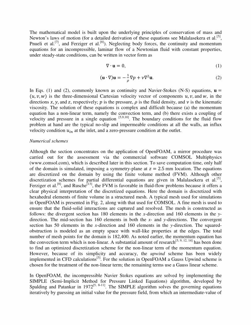
The mathematical model is built upon the underlying principles of conservation of mass and
Newton’s laws of motion (for a detailed derivation of these equations see Malalasekera et al.[5]
,
Pnueli et al.[7]
, and Ferziger et al.[8]
). Neglecting body forces, the continuity and momentum
equations for an incompressible, laminar flow of a Newtonian fluid with constant properties,
under steady-state conditions, can be written in vector form as
∇ ∙ u � 0, (1)
�u ∙ ∇�u � −
�∇� + �∇��. (2)
In Eqs. (1) and (2), commonly known as continuity and Navier-Stokes (N-S) equations, u �
��, �, �� is the three-dimensional Cartesian velocity vector of components �, �,and�, in the
directions �, �,and�, respectively; � is the pressure, � is the fluid density, and � is the kinematic
viscosity. The solution of these equations is complex and difficult because (a) the momentum
equation has a non-linear term, namely the convection term, and (b) there exists a coupling of
velocity and pressure in a single equation [5,9,10]
. The boundary conditions for the fluid flow
problem at hand are the typical no-slip and impermeable conditions at all the walls, an influx
velocity condition ��� at the inlet, and a zero-pressure condition at the outlet.
Numerical schemes
Although the section concentrates on the application of OpenFOAM, a mirror procedure was
carried out for the assessment via the commercial software COMSOL Multiphysics
(www.comsol.com), which is described later in this section. To save computation time, only half
of the domain is simulated, imposing a symmetry-plane at � � 2.5mm location. The equations
are discretized on the domain by using the finite volume method (FVM). Although other
discretization schemes for partial differential equations are given in Malalasekera et al.[5]
,
Ferziger et al.[8]
, and Rusche[13]
, the FVM is favorable in fluid-flow problems because it offers a
clear physical interpretation of the discretized equations. Here the domain is discretized with
hexahedral elements of finite volume in a structured mesh. A typical mesh used for simulations
in OpenFOAM is presented in Fig. 2, along with that used for COMSOL. A fine mesh is used to
ensure that the fluid-solid interactions are captured and resolved. The mesh is constructed as
follows: the divergent section has 180 elements in the x-direction and 160 elements in the y-
direction. The mid-section has 160 elements in both the x- and y-directions. The convergent
section has 50 elements in the x-direction and 160 elements in the y-direction. The squared-
obstruction is modeled as an empty space with wall-like properties at the edges. The total
number of mesh points for the domain is 182,400. As noted earlier, the momentum equation has
the convection term which is non-linear. A substantial amount of research[5, 9, 12, 14]
has been done
to find an optimized discretization scheme for the non-linear term of the momentum equation.
However, because of its simplicity and accuracy, the upwind scheme has been widely
implemented in CFD calculations[5]
. For the solution in OpenFOAM a Gauss Upwind scheme is
chosen for the treatment of the non-linear term; the remaining terms use a Gauss linear scheme.
In OpenFOAM, the incompressible Navier Stokes equations are solved by implementing the
SIMPLE (Semi-Implicit Method for Pressure Linked Equations) algorithm, developed by
Spalding and Patankar in 1972[5, 8-11]
. The SIMPLE algorithm solves the governing equations
iteratively by guessing an initial value for the pressure field, from which an intermediate-value of

(a) (b)
Figure 2. Typical meshing of the domain. (a) OpenFOAM. (b) COMSOL Multiphysics.
the velocity field is obtained from solution of the momentum equations. Velocity- and pressure-
correction terms are then calculated from the approximated velocity values given that the new
velocity values must satisfy the continuity equation. This process is repeated until the solution
has reached an acceptable predefined level of error (or tolerance). Detailed description of this
method can be found in Malalasekera et al.[5]
, Ferziger et al.[8]
, Patankar[10]
and Galpin et al.[11]
.
For the assessment of the results via COMSOL Multiphysics, the governing equations were
discretized on the domain and solved by the finite element method. In this technique, the
computational domain is divided into a set of discrete subdomains, denominated elements, each
with specific shape and mathematical properties; i.e., the approximation functions (and
corresponding coefficients) of a series expansion that describes the solution of the governing
equations. A weighted-integral process of the residual between the approximated and the original
equations over each element generates a set of algebraic relations among the unknown
parameters of the approximation, and hence, the solution by a matrix-vector operation. The
geometry is constructed using a three-dimensional mesh with quadrilateral elements along the
boundary and hexahedral elements inside the domain. To ensure accurate results while
maintaining a manageable CPU time, more dense meshing is using near all the wall boundaries.
For the construction of the mesh in COMSOL, 160 elements were used in the y-direction
throughout the domain, with exception of the region where the squared-obstruction is modeled,
where only 120 elements were used. A number of 173 elements were used the x-direction, giving
a total number of elements of 78240. The steady-state problem was solved by COMSOL with the
iterative scheme known as Generalized Minimum Residual Method (GMRES), for which the
relative tolerance was set to 10−6
. For both OpenFOAM and COMSOL several grids were tested
in order to ensure grid independence of the corresponding results.
Results and Analysis
The numerical results obtained from OpenFOAM are shown qualitatively in the form of velocity
fields in Fig. 3, and streamlines in Fig. 4, at the symmetry plane. On the other hand, the same
results are shown quantitatively, in terms of the streamwise velocity (x-direction), in Fig. 5. For
purposes of direct comparison, in the figures the OpenFOAM results are shown side-by-side with
the numerical solutions computed by COMSOL. From Figs. 3—5, it is clearly seen that, as
expected, the results obtained from OpenFOAM are very close to those of COMSOL, and

describe the fluid flow of water in the channel showing similar patterns for the velocity field and
the streamlines. Both numerical solutions present regions of recirculation due to the large slope
of the divergent section which produces an adverse pressure gradient, causing the flow to
separate and reverse its direction. Due to these recirculation areas at the development-flow
region of the channel, the mean velocity in the central region first accelerates until later
decelerating due to the presence of the squared-obstruction. Also expected are the flow
recirculation regions at the top and bottom edges of the object and at the region behind it. It is to
be noted that these recirculation effects are consistent with those obtained by the visualization
experiment presented in Fig. 7. It should also be noted that, although not shown here, the
recirculation effects obtained numerically in the diverging region of the channel, are absent in
the actual physical system. This is due to the fact that the experimental prototype contains a set
of veins that re-direct the flow to avoid flow separation in this region. This effect has an impact
on the flow downstream; thus, smaller recirculation regions would be expected as a consequence.
Although close, there are some differences between the results from the numerical schemes. The
results from COMSOL show a larger area of flow separation in the divergent inlet channel;
OpenFOAM also shows that effect, but to a lesser extent.
Figure 5 shows, quantitatively, that the numerical results from OpenFOAM and COMSOL
follow the same pattern and are very close. For purposes of comparison, plots of the x-
component of velocity at different cross-sections; i.e., at (a) 90 mm, which is the starting point of
the model insert; at (b) 99 mm, at the left boundary of the squared-obstruction; at (c) 130 mm,
(a)
(b)
Figure 3. Velocity field, x-component: (a) OpenFOAM (b)COMSOL Multiphysics.
(a)
(b)
Figure 4. Streamlines at the symmetry plane (z=2.5 mm). (a) OpenFOAM, (b) COMSOL.

(a)
(b)
Figure 5. Streamwise-component of the velocity at different cross-sections along the channel.
(a) OpenFOAM. (b) COMSOL.
which correspond to the plane located at midpoint of the model insert; and at (d) 150 mm, at the
recirculation zone are illustrated in this figure. From the figure it is observed that, in general, the
velocities in the x-direction obtained from COMSOL are slightly higher than those results
obtained by OpenFOAM. There are several possible explanations for the difference in the results
which include the difference in the discretization schemes and number of meshing points and the
type of interpolation methods used to obtain the velocity fields in the domain.
Experimental System and Analysis of Flow Visualization Results
FlowCoachTM
is an educational flow visualization and analysis system designed and produced by
Interactive Flow Studies Corp. to be used in a classroom or laboratory. The Flowcoach
visualization instrument, shown in Fig. 6, can be used with a variety of inserts containing
different obstruction geometries, allowing for the study of different flow phenomena in different
geometries. Neutrally-buoyant polyamide seeds (particles) are added to the water to enhance
flow visualization. The seeds reflect light emitted by attached LED lights, giving the students an
excellent opportunity to visually examine the effects the obstruction has on the flow. For the
problem being analyzed, the flow rate passing through the channel is set at 0.4 gpm which gives
a uniform inlet velocity of 0.1869 m/s (in the x-direction).
Flowcoach uses particle image velocimetry (PIV), a technique used to obtain instantaneous
velocities of the flow at given points in space. A mounted camera captures a short video of the
flow around the square obstruction (other geometries are available) that is decomposed into
individual frames. The PIV technique compares sequential frames to approximate the distance a
group of particles travels over an area. Using this approximated distance and the time between
each frame (determined from the video capture speed), the instantaneous velocity is determined
at a point. This technique is repeated to analyze the entire region and the result is the
instantaneous velocity vector field. Though Flowcoach provides students with opportunities for
visual appreciation and an excellent qualitative analysis of the flow, several factors that might
contribute to poor results include: the camera settings such as positioning and capture speed,
-0.04
0
0.04
0.08
0.12
0.16
0.2
0 10 20 30 40 50 60 70 80 90
U V
elo
city
, m
/s
Vertical position, mm
U (X-direction) Velocity Profile
x=90 x=99 x=130 x=150
-0.04
0
0.04
0.08
0.12
0.16
0.2
0 10 20 30 40 50 60 70 80 90
U V
elo
city
, m
/s
Vertical Position
U (X-direction) Velocity Profile
x=90 x=99 x=130 x=150

Figure 6. FlowCOACH by Interactive Flow Studies Corporation.
lighting, quantity of seeds, overall quality of video captured, correct adjustment of inputs and the
efficiency of the integrated PIV software.
Experimental tests of the flow around the aforementioned squared-obstruction were carried out
using FlowCOACH. The value of the inlet velocity for the experiment corresponds to that
considered for the numerical simulations ��� � 0.1967 m/s. Figure 7a shows the flow field in
terms of the streamlines around the squared-obstruction. From this image the regions where the
fluid is stagnant at the leading edge of the object, the development of the boundary layer and
consequent flow separation at the top and bottom surfaces, and the recirculation bubble at the
trailing edge of the obstruction can be clearly seen. A qualitative comparison of the experimental
observations to the OpenFOAM numerical simulations, on the other hand, is shown in Fig. 7b.
The figure reveals that the solution obtained via CFD depicts, fairly accurate, the true physical
characteristics of the flow in the region around the object. By looking closer, one can perceive
some slight differences between the superimposed numerical solution and the reflected neutrally-
buoyant particles. These differences are thought to be due to the fact that the numerical model
has been constructed without taking into account the directional veins that the physical
prototype; named, the model insert, contains to eliminate the recirculation zones at the divergent
region of the channel, which are shown in the numerical solutions of Figs. 3 and 5.
Concluding Remarks
Applications of fluid mechanics are found in many areas of civil and mechanical engineering.
Thus, an in-depth understanding of FM is a pre-requisite to engineers working in these fields.
This paper proposes a new approach to teaching fluid mechanics concepts that integrates
computation fluid dynamics (CFD) simulations to the conventional theory/laboratory method.
While analytical solutions that are taught in theory-focused lessons can be applied to elementary
problems, understanding and design of more advanced systems cannot be achieved through these

(a)
(b)
Figure 7. Flow visualization of the flow field. (a) Original image. (b) OpenFOAM superimposed
streamlines.
solutions alone. Testing and measurements of experimental settings are often an effective
alternative. In most cases, however, accurate measurements of fluid pressure and velocity fields
are either very expensive or impossible. In these cases, one can only rely on validated numerical
solutions, such as CFD simulations. Through this integrated approach, students learn the
benefitsof each method and how they can be applied in the design of complex fluid-flow
systems. An open-source software known as OpenFOAM was the CFD software of choice. In
addition to being free, the large number of pre-defined solvers included and the capability for
user-defined solvers make OpenFoam suitable for educational and research purposes.
Comparison of OpenFOAM with COMSOL, a widely-used commercial software, has proven
OpenFOAM to be very accurate, reliable and easy to implement. Experimental analysis was
performed using a flow visualization device named FlowCoach. A qualitative comparison of
FlowCoach and OpenFoam results indicates that the CFD results are fairly accurate. The
proposed integrated approach is currently being implemented at California State University Los
Angeles. It is expected that it will significantly enhance student learning of abstract and complex
concepts of fluid mechanics.
Acknowledgements
This material is based upon work supported by the National Science Foundation NSF-SBIR
phase II grant (IIP-0844891), and partially supported by NSF-funded CREST center (HRD-
0932421). Any opinions, findings, and conclusions or recommendations expressed in this
material are those of the author(s) and do not necessarily reflect the views of the National
Science Foundation.

References
[1] Friedrich, J. “Object-oriented design and implementation of CFDLab: a computer assisted learning tool for
fluid dynamics using dual reciprocity boundary element methodology.” Computers and Geosciences, Volume 25,
1999, pp. 785-800.
[2] Stern, F., Xing, T., Yarbrough, D.B., Rothmayer, A., Rajagopalan, G., Otta, S.P., Bhaskaran, R., Smith, S.,
Hutchings, B., Moeykens, S. “Hands-on CFD educational interface for engineering courses and laboratories.”
Journal of Engineering Education. Volume 95, No. 1, 2006, pp. 63-83.
[3] Fraser, D.M., Pillay, R., Tjatindi, L., Case, J.M. “Enhancing the learning of fluid mechanics using computer
simulations.” Journal of Engineering Education. Volume 96, No. 4, 2007, pp. 381-388.
[4] Tannehill, J.C., Anderson, D.A., Pletcher, R.H. Computational Fluid Mechanics and Heat Transfer. 2nd
Ed.
Taylor & Francis. 1997. Philadelphia, PA.
[5] Malalasekera, W., Verseeg, H.K. An Introduction to Computational Fluid Dynamics: The finite volume method.
Longman Scientific & Technical. 1995. New York, NY.
[6] Medina, R., Okcay, M., Menezes, G., Pacheco-Vega, A. “Implementation of Particle Image Velocimetry in the
Fluid Mechanics Laboratory.” In: Proceedings of the 2011 PSW American Society for Engineering Education
Conference, Fresno, CA, USA, 2011, pp. 42-50.
[7] Pnueli, D., Gutfinger, C. Fluid Mechanics. Cambridge University Press. 1992. Cambridge, UK.
[8] Ferziger, J. H., Peric, M. Computational Methods for Fluid Dynamics, 3rd Ed. 2001. Springer, New York,
NY.
[9] Jasak, H. “Error Analysis and Estimation for the Finite Volume Method with Applications to Fluid Flows”,
Ph.D. Thesis, Imperial College, London, 1996
[10] Patankar, S.V. “A calculation procedure for two-dimensional elliptic situations.” Numerical Heat Transfer,
Volume 4, 1981, pp. 409-425.
[11] Galpin, P.F., Van Doormaal, J.P., Raithby, G.D. “Solution of the incompressible mass and momentum
equation by application of a coupled equation line solver.” International Journal for Numerical Methods in Fluids,
Volume 5, 1985, pp. 615-625.
[12] Galpin, P.F., Raithby, G.D. “Treatment of non-linearities in the numerical solution of the incompressible
Navier-Stokes equations.” International Journal for Numerical Methods in Fluids, Volume 6, 1986, pp. 409-426
[13] Rusche, H. “Computational fluid dynamics of dispersed two-phase Flows at High Phase Fractions,” Ph.D.
Thesis, Imperial College, London, 2002
[14] Zhao, Y., Zhang, B. “A high-order characteristics upwind FV method for incompressible flow and heat
transfer simulation on unstructured grids.” Computer Methods in Applied Mechanics and Engineering, Volume
190, 2000, pp. 733-756.