On the Importance of Viscoelastic Response

Consideration in Structural Design Optimization

Kai A. Jamesa, Haim Waismanb

aUniversity of Illinois at Urbana-Champaign, Department of Aerospace Engineering,Urbana, Illinois, United States; tel: 217-300-3270; fax: 217-244-0720;

kaijames@illinois.edubColumbia University, Department of Civil Engineering and Engineering Mechanics,

New York, New York, United States

Abstract

In this paper we present a series of mathematical proofs that demonstratethe importance of accounting for viscoelastic effects in structural optimiza-tion algorithms. Focusing specifically on mass minimization problems withstiffness and deflection constraints, we show that standard techniques basedon linear elastic analysis overestimate the long-term stiffness of the struc-ture, leading to designs that become infeasible after sustained loading due toviscoelastic creep. Conversely, assuming maximum creep deflection, whichalso allows for linear analysis, leads to an overly conservative design that isunnecessarily heavy and therefore suboptimal. We prove both propositionsfor both constant and time-varying load histories. We also present proofs forgeneralized continuum mechanics problems as well as for a finite element for-mulation, which can be applied to any arbitrary geometry. Lastly, we presenttwo numerical examples in which the conclusions derived in the proofs areverified empirically.

Keywords: structural optimization; viscoelasticity; creep deformation;finite element analysis

1. Introduction

Viscoelasticity is the property by which solid materials exhibit time-dependent responses when subject to sustained loading. While many en-gineering materials are known to have significant and observable viscoelasticbehavior, particularly when operating at high temperatures, most structural

Preprint submitted to Optimization and Engineering April 28, 2016

design optimization procedures fail to take this property into account, andinstead treat the structural material properties as being independent of time.Because of the time-dependent nature of viscoelastic materials, they are oftenused in structural damping applications, and there have been a number ofstudies on viscoelastic design optimization of structures subject to dynamicloading [1, 2, 3, 4, 5, 6]. However, few have tackled the problem of struc-tural design while accounting for unwanted viscoelastic effects such as creepdeformation. In this paper, we explore the design of structures subject tosustained loading that is either constant, or varies on a time scale that is slowenough that all inertial effects are negligible. When subject to these typesof loads, viscoelastic structures exhibit creep deformation in which the de-flection of the structure increases gradually, with the rate of increase slowingdown over time.

A recent study by the authors [7] explored the use of viscoelastic analysisin topology optimization algorithms for designing structures, while takinginto account undesirable creep effects, in order to improve long-term struc-tural performance. Through several numerical examples, it was shown thatstructures that were designed under the assumption of linear elasticity, be-came infeasible and failed to meet the design requirements when the struc-ture’s long-term performance was evaluated using a linear viscoelastic model.Similarly, the examples showed that when the authors attempted to accountfor viscoelastic effects by implementing a simplified worst-case viscoelasticmodel, the resulting structure was over-designed and was therefore subop-timal. The solution was to incorporate time-dependent viscoelastic analysisinto the structural optimization algorithm, in order to achieve a structurethat was both feasible and optimal for the specific load duration or oper-ating time for which the structure was to be designed. The current paperextends upon the previous study by presenting formal mathematical proofsof the observations and conclusions of that study. These proofs further high-light the importance of accounting for viscoelastic effects in the design ofstatic structures comprised of viscoelastic material.

2. The Linear Viscoelastic Model

In the current paper, as well as in the previous study [7], the material isassumed to exhibit linear viscoelasticity. From the principle of Boltzmannsuperposition, one can deduce the following viscoelastic stress-strain relationfor a time-varying axially applied stress, evaluated at time t .

2

σ(t) =

∫ t

0

E(t− s)∂ε(s)∂s

ds. (1)

where E is the relaxation modulus or relaxation function, and s is a dummyvariable representing the domain over which the integral is evaluated . Thisfunction is an intrinsic property of the material and is typically determined byfitting experimental data [8]. When used to describe one-dimensional axialloading, the parameter E is referred to as the extensional relaxation function.This quantity is analogous to the elasticity modulus used to describe stiffnessin elastic materials. Alternatively, one can describe the viscoelastic behaviorof a material using the creep compliance function, D, which is the inverse ofthe relaxation function. When a viscoelastic material is subject to constantloading the strain history of the material response follows the path of thecreep compliance function. The two functions are related to one another viathe following equation.

∫ t

0

D(t− s)∂E(s)

∂sds = 1 (2)

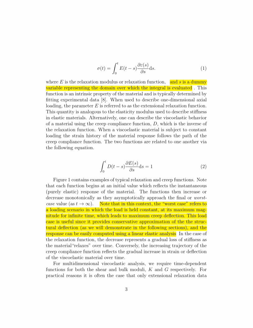
Figure 1 contains examples of typical relaxation and creep functions. Notethat each function begins at an initial value which reflects the instantaneous(purely elastic) response of the material. The functions then increase ordecrease monotonically as they asymptotically approach the final or worst-case value (as t→∞). Note that in this context, the “worst case” refers toa loading scenario in which the load is held constant, at its maximum mag-nitude for infinite time, which leads to maximum creep deflection. This loadcase is useful since it provides conservative approximation of the the struc-tural deflection (as we will demonstrate in the following sections), and theresponse can be easily computed using a linear elastic analysis In the case ofthe relaxation function, the decrease represents a gradual loss of stiffness asthe material“relaxes” over time. Conversely, the increasing trajectory of thecreep compliance function reflects the gradual increase in strain or deflectionof the viscoelastic material over time.

For multidimensional viscoelastic analysis, we require time-dependentfunctions for both the shear and bulk moduli, K and G respectively. Forpractical reasons it is often the case that only extensional relaxation data

3

0 t

E(t)

t0

E0

E∞

(a) Relaxation function

0 t

D(t)

t0

D0

D∞

(c) Creep function

Figure 1: Examples of typical relaxation and creep functions

are available, and therefore one must extrapolate this data to obtain shearand bulk modulus functions [9]. Depending on the material, the viscoelasticbehavior in shear and in bulk may differ significantly, however a commonapproach is to assume synchronicity in between the two functions [10, 11]],so that

K(t) = βG(t). (3)

where β is a constant scalar multiplier. Under this assumption, the fullviscoelastic response of the material can be captured by a single relaxationmodulus [12]. Therefore it is convenient to employ to a constitutive lawbased on the Young’s modulus and the Poisson ratio, since ν reduces to aconstant ν = ν0, and the extensional relaxation modulus, E(t) can be treatedas being mathematically equivalent to the time-dependent Young’s modulus,EY. For a general two- or three-dimensional problem, the linear viscoelasticstress-strain relation is given by

σ(t) =

∫ t

0

C(t− s)∂ε(s)∂s

ds. (4)

where σ and ε are the stress and strain tensors respectively, and C(t) is

the time-dependent elasticity tensor given by E(t)E0

C0, where C0, is the ini-tial (maximum stiffness) elasticity prior to the onset of relaxation . Note

4

that this relation applies specifically to linear elastic materials that obey theBoltzmann superposition principle. For simplicity the proofs that follow arebased this synchronous viscoelastic model.

3. Viscoelastic Modeling and Structural Optimization

The previous paper [7] investigated structural optimization problems inwhich the objective was to minimize the structural mass, subject to a con-straint on the maximum deflection due to creep measured at some targettime t∗. The optimization problem can be written mathematically as follows

minx

Ne∑e=1

aexe

subject to: u(t∗) ≤ u∗, (5)

where xe are generic structural design variables that could represent mate-rial densities in the case of topology optimization problems, or cross-sectionalareas in the case of discrete truss structures. The coefficients ae represent spe-cific geometric properties of the structural elements. In the case of topologyoptimization, ae represents the element volume, and in the case of discretetruss elements, ae represents the element length, so that, when multipliedby the design variables, the resulting product is proportional to the massof the element. The variable u represents the local displacement at a givenlocation, and this value is constrained so that it does not exceed the targetdisplacement u∗.

In the previous study, it was observed that, when solving the above designproblem, assuming linear elasticity leads to an insufficiently stiff structure,whose deflection overshoots its target value once viscoelasticity is taken intoaccount. Similarly, design based on a worst-case scenario assumption causesthe optimizer to over-design the structure, making it unnecessarily heavy.Here we offer a mathematical proof that this observation will hold in gen-eral for any minimum-mass optimization procedure involving isotropic linearviscoelastic material. These two extreme cases (elastic and worst-case) aresignificant benchmarks, since both can be evaluated rapidly using linear elas-tic analysis. However, through the proofs presented below, we demonstratethat both techniques are flawed since they yield structural designs that areeither infeasible, or suboptimal.

5

In order to state the problem mathematically, we express the viscoelasticdisplacement, u, as a function of the design variable vector x, and the time,t. Note that u is a scalar quantity corresponding to the displacement atthe specific location (or degree of freedom) at which we seek to enforce theconstraint during the optimization. Furthermore, let xelastic represent thestructure that is optimized so that its deflection meets the target deflectionvalue, u∗, when analyzed under the assumption of elasticity. Therefore

u(xelastic, t0) = u∗ (6)

where t0 is the initial time at which the load is first applied. Similarly, letxworst represent the structure that is optimized so that its deflection meetsthe target deflection value, u∗, under the worst-case assumption (i.e. t→∞and F(t) = Fmax for all t, where Fmax is the maximum value reached by theactual time-dependent force history function). Therefore

u(xworst,∞)|F=Fmax= u∗ (7)

Lastly, let xvisc represent the structure that is optimized using viscoelasticanalysis so that

u(xvisc, t∗) = u∗, for t0 < t∗ < t∞ (8)

Where t∗ ∈ (t0,∞) is the critical time for which the structure is to be de-signed. Using these definitions, we shall prove the following inequalities.

|u(xworst, t∗)| < |u∗| < |u(xelastic, t

∗)|, for t∗ > t0 (9)

Note that in the above inequality, the elastic design and worst case designare evaluated based on their respective deflections at time t∗, using a time-dependent viscoelastic analysis in which t∗ − t0 is some finite, non-zero timeduration. Note also that in the limiting case where t∗ = t0 the viscoelasticanalysis is equivalent to an elastic analysis so that u(xelastic, t

∗) = u∗. Inthe remaining subsections we prove this relation for both constant and time-varying loads.

6

4. Constant Loading

In the case of constant loading, the proof is trivial. One need simplyobserve that

u(x, t) = u(x, t0)D(t)

D0

, withD(t)

D0

> 1 for all t > 0. (10)

Note that this statement makes no assumptions about the geometry or dis-cretization of the problem. From here, one can easily deduce that |u(xelastic, t

∗)| >|u∗|, for t∗ > t0. Therefore, the full proof, along with the proof of the firsthalf of the general proposition pertaining to the worst-case design are left asexercises for the reader.

5. Time-Varying Loads

5.1. One-Dimensional Problems

In this section we derive analogous proofs for a general, time-varying pro-portional load. We initially derive the proofs for a simple one-dimensionalaxial load problem, and in Section 5.2 we show how these proofs can be ex-tended to apply to any arbitrary geometry using a finite element formulation.In the case of a one-dimensional geometry with axial loading, the load can beexpressed using the scalar σ, which represents the applied stress. Similarly,the strain state can be captured using the scalar ε. Note that we restrict theproofs to loads in which the force does not change direction (i.e. σ(t) > 0 forall t > t0), which is a reasonable assumption for many support structures.For all loads satisfying this description, we wish to prove that the actualviscoelastic displacement for a structure optimized based on a linear elasticmodel is greater than the target displacement for which the structure wasdesigned. Similarly, we shall prove that for a structure optimized using aworst-case analysis, the actual viscoelastic displacement is smaller than thetarget displacement, u∗, for which the structure was designed, thus makingthe design suboptimal. For increased simplicity, we make use of the factthat the axial displacement is directly proportional to the axial strain (i.e.u = εL, where L is the axial length of the undeformed structure. Thereforethe general proposition can be written in terms of the axial strains as follows.

ε(xworst, t∗) < ε∗ < ε(xelastic, t

∗) (11)

7

By proving the above inequality, we implicitly prove the proposition ex-pressed in 9. All proofs assume linear viscoelasticity and therefore the Boltz-mann superposition equation applies.

From the known characteristic of the the relaxation function, we canderive two properties that will assist in the proof. First we note that sinceE is a monotonically decreasing function (see Fig. 1a), we can assert thefollowing.

lemma 1© : if t1 < t2, then E(t1) > E(t2) (12)

Secondly, from the Boltzmann equation 1, one can deduce the following

lemma 2© : if σ(t) ≥ 0 for all t, then ε(t) ≥ 0 for all t (13)

Although this latter observation appears to be intuitive, its proof is non-trivial. Therefore, below we present a proof, which uses integration by parts.We begin with the complementary form of the Boltzmann superpositionequation in which the time-dependent strain function ε(t) is expressed asa function of the stress history and the creep compliance function D(t) asfollows.

ε(t) =

∫ t

0

D(t− s)∂σ(s)

∂sds (14)

Integrating by parts, we obtain

ε(t) = [D(t− s)σ(s)]t0 −∫ t

0

[∂

∂sD(t− s)

]σ(s)ds (15)

The first term in the above expression must be greater that zero since bothD(t) and σ(t) are positive for all times t. Turning to the integral term, wenote that

∂

∂sD(t− s) =

∂D(r)

∂r

∂r

∂s, where r = t− s; (16)

8

From Figure 1b, we see that ∂D(r)∂r

> 0 for all r, and since ∂r∂s

= −1, we candeduce that ∂

∂sD(t − s) < 0 for all s and t. Also, since σ(s) is strictly

positive for all s, we have shown that the second term in Eqn. 15 is alsopositive. Therefore ε(t) > 0 for all t, and the proof of Lemma 2 is complete.

From here, we proceed to the latter portion of the general proposition(11), which pertains to designs optimized using linear elasticity. We mustshow that

ε∗ < ε(xelastic, t∗). (17)

According to linear elasticity, the stress-strain relation is given by

σ(t∗) = E0εelastic(xelastic, t∗), (18)

For any structure designed to satisfy the deflection constraint given in Eqn.5, under the assumption of linear elasticity, the elastic strain will be equalto the target strain, i.e. εelastic(xelastic, t

∗) = ε∗. Therefore, we can deduce arelationship between the target strain, ε∗, and the actual viscoelastic strain,ε, of the structure represented by xelastic as follows.

E0ε∗ = σ(t∗) =

∫ t∗

0

θ(s)∂ε(s)

∂sds

⇒ ε∗ =

∫ t∗

0

θ(s)

E0

∂ε(s)

∂sds (19)

=

∫ t∗

0

∂ε(s)

∂sds−

∫ t∗

0

(1− θ(s)

E0

)∂ε(s)

∂sds

= ε(t∗)−∫ t∗

0

(1− θ(s)

E0

)∂ε(s)

∂sds (20)

Note that in the above equations, we have omitted the x variable for improvedclarity, however it is implied above, as well as for the remainder of the proof,that ε(t∗) = ε(xelastic, t

∗). Rearranging to isolate the viscoelastic strain term,ε(t∗), and integrating by parts we obtain

9

ε(t∗) = ε∗ +

[(1− θ(s)

E0

)ε(s)

]t∗0

−∫ t∗

0

(−∂θ(s)

∂s

)ε(s)ds

= ε∗ +

(1− θ(t∗)

E0

)ε(t∗) +

∫ t∗

0

∂θ(s)

∂sε(s)ds (21)

Note that, as before, the term(

1− θ(0)E0

)ε(0) vanishes since ε(0) = 0. Since

E0 represents the peak value of both E(s) and θ(s), we know that θ(s)E0≤ 1,

therefore(

1− θ(s)E0

)≥ 0. Also, from lemma 2, ε(s) > 0 for all s > 0. Lastly

∂θ(s)∂s

> 0, since θ(s) is a monotonically increasing function. Therefore, wecan write

ε(t∗) = ε∗ + Π, where Π > 0, (22)

which implies that ε(xelastic, t∗) > ε∗, and thus the proof is complete.

The portion of the proposition pertaining to the worst-case design (i.e.ε(xworst, t

∗) < ε∗) is solved in two parts. Here we introduce an intermedi-ate analysis method in which the applied force remains constant at σ(t) =max(σ), for all t > 0, however we solve for the viscoelastic strain at t∗ usinga time-dependent analysis. This approach is hereafter referred to as a partialworst case analysis, and the strains obtained by this method shall be denotedusing ε. Therefore we seek to prove that

ε(xworst, t∗) ≤ ε(xworst, t

∗) < ε∗. (23)

Note that since all strain values apply to the worst case design, xworst, weagain omit the x variable, so it should be understood that for the remainderof the proof ε(t) = ε(xworst, t). The first part of the above inequality (i.e.ε(t∗) ≤ ε(t∗)), can proved simply by expressing both strain quantities in theform given in Eqn. 15, which we derived earlier using integration by parts.

ε(t) =1

E0

σ(t) +

∫ t

0

1

[θ(s)]2∂θ(s)

∂sσ(s)ds (24)

ε(t) =1

E0

σ(t) +

∫ t

0

1

[θ(s)]2∂θ(s)

∂sσ(s)ds (25)

10

Noting that σ(t) ≥ σ(t) for all t > 0 (from the definition of σ), one candeduce from inspection that ε(t∗) ≥ ε(t∗), therefore the proof is complete.

For greater understanding, we present an alternative proof based onmathematical induction. We begin by writing the Boltzmann form of time-dependent applied stress function, σ, and the partial worst-case stress func-tion, σ, with the integrals expressed as a Riemann sum, in which the differ-ential time increment ds is replaced by a finite time step ∆t.

σ(t∗) = lim∆t→0

nt∑i=1

E(t∗ − ti)∆εi (26)

σ(t∗) = lim∆t→0

nt∑i=1

E(t∗ − ti)∆εi, (27)

Where nt = t∗/∆t and ∆εi > ε(ti)− ε(ti−1). Since σ(t) ≥ σ(t) for all t > 0,we can further assert that

lim∆t→0

nt∑i=1

E(t∗ − ti)∆εi ≤ lim∆t→0

nt∑i=1

E(t∗ − ti)∆εi (28)

Let us now assume that the above relation holds true for some consistentdiscretization of the time domain, which uses a finite time step, ∆t > 0. Wecan therefore omit the limit term to obtain

nt∑i=1

E(t∗ − ti)∆εi ≤nt∑i=1

E(t∗ − ti)∆εi, (29)

which holds for all values of nt. From here we must prove that ε(tnt) ≤ ε(tnt),or equivalently

nt∑i=1

∆εi ≤nt∑i=1

∆εi, (30)

in order to show that ε(t∗) ≤ ε(t∗). We now proceed with the proof bymathematical induction. For the base case, we prove the above statementwith nt = 1. From Eqn. 29 we have

11

E(0)∆ε1 ≤ E(0)∆ε1. (31)

From here, it is trivial to deduce that ε(t1) ≤ ε(t1), therefore the base caseis proven. To prove that Eqn. 30 holds for any number of terms nt we firstassume that it holds for nt = k. Therefore

k∑i=1

∆εi ≤k∑i=1

∆εi. (32)

Now, based on this assumption, we prove that Eqn. 30 must also hold fornt = k + 1. From Eqn. 29, we have

k+1∑i=1

E(t∗ − ti)∆εi ≤k+1∑i=1

E(t∗ − ti)∆εi. (33)

We now decompose both sums as follows.

k+1∑i=1

[E(0)− (E(0)− E(tk+1 − ti))] ∆εi ≤k+1∑i=1

[E(0)− (E(0)− E(tk+1 − ti))] ∆εi

(34)

Noting that tk+1 − ti = (k + 1− i)∆t the inequality becomes

E(0)k+1∑i=1

∆εi−k+1∑i=1

[E(0)− E((k + 1− i)∆t)] ∆εi

≤ E(0)k+1∑i=1

∆εi −k+1∑i=1

[E(0)− E((k + 1− i)∆t)] ∆εi (35)

In the latter summation on either side of the inequality, the final term in thesummation (i = k + 1) vanishes. Therefore, omitting that k + 1 term andrearranging the remaining terms in the summation, we arrive at

12

E(0)k+1∑i=1

∆εi−k∑i=1

[(E((k − i)∆t)− E((k + 1− i)∆t)

) i∑j=1

∆εj

]

≤ E(0)k+1∑i=1

∆εi −k∑i=1

[(E((k − i)∆t)− E((k + 1− i)∆t)

) i∑j=1

∆εj

](36)

Rearranging to isolate the ε(tk+1) and ε(tk+1) terms, we obtain

E(0)

(k+1∑i=1

∆εi −k+1∑i=1

∆εi

)

≥k∑i=1

[(E((k − i)∆t)− E((k + 1− i)∆t)

) i∑j=1

(∆εj −∆εj)

](37)

From the assumption, we know that ∆εj−∆εj > 0 for all j up to j = k. Also,from lemma 1 (Eqn. 12), we know that E((k− i)∆t)−E((k+ 1− i)∆t) > 0for all values of i and k. Lastly, we know that E(0) > 0, therefore we canconclude that

k+1∑i=1

∆εi −k+1∑i=1

∆εi ≥ 0

⇒ ε(tk+1) ≤ ε(tk+1) (38)

By mathematical induction, this proves that ε(ti) ≤ ε(ti) for all i > 0, andtherefore the proof is complete.

To prove the second half of the proposition in 23, (i.e. ε(xworst, t∗) < ε∗),

we begin with the definition of the worst-case design, xworst, which is definedas x such that the viscoelastic strain satisfies ε(x, t∞) = u∗. However we alsoknow, from Eqn. 10, that the worst case strain is computed using

ε(xworst, t∞) =D∞D0

ε0 =D∞D0

σmax

E0

, (39)

13

where ε0 is the elastic strain due to the peak applied stress, σmax. Thereforefrom the definition of xworst, we can write

ε∗ =D∞D0

σmax

E0

, (40)

We must now express the above equation in terms of the extremal relax-ation coefficients, E0 and E∞. This is achieved by using Laplace analysis.Applying a Laplace transformation to Eqn. 2 leads to

D(ξ) =1

ξ2E(ξ), (41)

where E and D are the Laplace transforms of the relaxation and creep com-pliance functions respectively, and ξ is the transform parameter. From theknown properties of Laplace transforms, we can write

D(t∞) = limξ→0+

ξD(ξ) = limξ→0+

1

ξE(ξ). (42)

Furthermore, any relaxation function can be described using a Prony seriesexpression of the form

E(t) = E∞ +

Np∑j=1

Eje−t/τj , (43)

where Np is the number of Prony terms in the series, and the coefficientsEj and τj, are constants selected to fit the Prony series function toexperimental results. Transforming the Prony series expression for E(t) intothe Laplace domain, we obtain

D(t∞) = limξ→0+

1

ξ(E∞ξ

+∑Np

j=1τjEj

τjξ+1

)=

1

E∞(44)

14

Using a similar process, one can show that D0 = 1/E0. Inserting theseidentities into Eqn. 40, we obtain

ε∗ =σmax

E∞, (45)

From the definition of the partial worst-case strain, ε, we know that

σmax =

∫ t∗

0

E(t∗ − s)∂ε(s)∂s

ds. (46)

Therefore we have

ε∗ =

∫ t∗

0

E(t∗ − s)E∞

∂ε(s)

∂sds

=

∫ t∗

0

∂ε(s)

∂s+

∫ t∗

0

(E(t∗ − s)E∞

− 1

)∂ε(s)

∂sds

= ε(t∗) +

∫ t∗

0

(E(t∗ − s)E∞

− 1

)∂ε(s)

∂sds (47)

Since E(t) > E∞ for all t, E(t∗−s)/E∞−1 > 0. It is also clear that ε(s) is amonotonically increasing function of s, since ε is the strain due to a constantapplied load of σmax. Therefore ∂ε(s)

∂s> 0 for all s. We can now write

ε∗ = ε(xworst, t∗) + Π, where Π > 0

⇒ε(xworst, t∗) < ε∗, (48)

Combining Eqn. 48 and 38, we get ε(xworst, t∗) < ε∗, and therefore the proof

is complete.This proves conclusively that the worst-case approach employed in the

examples provides a reliable upper bound on all possible deflections. It alsoshows that although this approach is computationally inexpensive (since theworst-case analysis requires the solution of just one linear system, similarto the elastic case), the actual viscoelastic deflection will be less than thetarget deflection value, which, as we showed earlier, results in a suboptimaldesign. Similarly, it has been shown that assuming linear elasticity leads toan infeasible structure that is insufficiently stiff, and therefore exceeds thetarget deflection. The performance of the optimal viscoelastic design will bebound on either side by these two extreme cases.

15

5.2. Extension to Multi-Dimensional Problems Using Finite Element Anal-ysis

The proofs presented in the previous section apply narrowly to the one-dimensional case involving a linear viscoelastic structure subject to unidi-rectional axial loading. However, in practice, most computational structuraloptimization methods involve two- or three dimensional structures with com-plex geometries, and which are modeled using finite element analysis, or someother form of discretization. In the current section, we show how the under-lying derivations for each of the proofs presented earlier, can be adapted toapply to two-and three-dimensional problems of arbitrary geometry. Specifi-cally we derive a proof of the proposition u(xelastic, t

∗) > u∗ for a generalizedstructure of arbitrary geometry and dimension using a generic finite elementformulation (note that since all equations in this section pertain to the elasticdesign xelastic, we hereafter omit the x variable, as was done in the previoussection). Derivation of the finite element analogs of the remaining proofspertaining to the worst case design, are left as an exercise for the reader.

For the general problem, we restrict the applied loads to the class ofproportional loads, meaning only the load magnitude varies with time, whilethe load pattern or profile remains constant. Mathematically this impliesthat all applied loads f(X, t) must satisfy

f(X, t) = α(t)f(X), X ∈ Rd, d ∈ 2, 3 (49)

where the variable X represents the spatial coordinate in two- or three-dimensional space, and α(t) is a scalar function indicating the relative mag-nitude of the applied force at time t. In finite element terms all applied forcescan be represented by

F(t) = α(t)F0 (50)

where F is the consistent force vector, and F0 is a constant vector describingthe load pattern. As in the previous section, we again restrict the appliedforces so that α(t) ≥ 0 for all t. Finally, we require that all loads be con-centrated loads that can be represented as single point loads in the finiteelement model (it is assumed that the deflection constraint is evaluated atthe location of the applied load). This restriction is necessary since the gen-eral proposition we seek to prove does not hold in general for all distributed

16

and multi-point loads. Under the generic finite element formulation, all ap-plied stresses, σ(t), from Section 5.1 are replaced with applied forces F(t)and all viscoelastic strains, ε(t) are replaced with viscoelastic displacementsu(t). Using a derivation similar to that which was used to prove lemma 2(Eqn. 13) above, it can be shown that

if α(t) ≥ 0 for all t, then u(t) > 0 for all t > 0 (51)

We begin by expressing the structure’s equilibrium equation in genericfinite element terms using a semi-discrete FEM form in which the spatialdomain is discretized, but the time domain remains continuous. We firstnote that

fe(t) =

∫Ωe

BTσ(t)dV

=

∫ t

0

∫Ωe

BTC(t− s)∂ε(s)∂s

dV ds (52)

where fe is the vector of applied nodal forces corresponding to element e,Ωe is the volume occupied by element e, and B is the strain displacementmatrix for element e. In the second line above, we have substituted thegeneral Boltzmann formula for the internal stress tensor, σ, (Eqn. 4). Thestrain displacement matrix is defined such that, ε = Bue, where ue is thevector of nodal displacements for element e. Therefore we can write

fe(t) =

∫ t

0

∫Ωe

BTC(t− s)B∂ue(s)∂s

dV ds

=

∫ t

0

ke(t− s)∂ue(s)

∂sds, (53)

where ke is the element stiffness matrix, which depend on t due to viscoelas-ticity, and can be computed using

ke =

∫Ωe

BTC(t− s)BdV. (54)

17

When we combine the equilibrium equations from all elements throughthe process of assembly, we arrive at the following global equilibrium equa-tion.

F(t) =

∫ t

0

K(t− s)∂u(s)

∂sds, (55)

where u is the global vector of nodal displacements. The viscoelastic dis-placement used to evaluate the constraint, is given by

u = LTu, (56)

where LT is the unit basis vector whose entries are zero except in the locationcorresponding to the node where the displacement is constrained (i.e. LT =[0 ... 0 1 0 ...0]T). Using this finite element formulation, we seek to provethat u(xelastic, t

∗) > u∗, where u∗ is the target displacement specified in thedesign optimization problem.

The elastic deflection, u0(xelastic, t∗), is obtained by solving the following

linear elasticity equation

F(t∗) = K0(xelastic)u0(xelastic, t∗), (57)

where K0(xelastic) is the global stiffness matrix corresponding to the designdescribed by xelastic at time t = 0. Note that since all variables used in theremainder of the proof correspond to the design x = xelastic, we hereafteromit the x value in all subsequent equations for increased clarity. Combiningequations 55 and 57, we can equate the two expressions for F(t∗) as follows.

K0u0(t∗) =

∫ t∗

0

K(t− s)∂u(s)

∂sds, (58)

Multiplying both sides of the equation by LK−10 , we obtain

u0(t∗) =

∫ t∗

0

E(t− s)E0

∂u(s)

∂sds, (59)

18

Now recall that the elastic design, xelastic, corresponds to the structure thatis designed so that, when evaluated based on the assumption of elasticity,its deflection satisfies the constraint u0(xelastic, t

∗) = u∗. Therefore we canreplace the quantity u0(t∗) above with the target deflection value, u∗. Fornotational brevity, we also re-introduce the variable θ(s) = E(t∗ − s). Con-sequently Eqn. 59 becomes

u∗ =

∫ t∗

0

θ(s)

E0

∂u(s)

∂sds

=

∫ t∗

0

∂u(s)

∂sds−

∫ t∗

0

(1− θ(s)

E0

)∂u(s)

∂sds (60)

= u(t∗)−∫ t∗

0

(1− θ(s)

E0

)∂u(s)

∂sds

As in the analogous proof from the previous section, we now rearrange toisolate the variable u(t∗), and integrate by parts to obtain

u(t∗) = u∗ +

[(1− θ(s)

E0

)u(s)

]t∗0

−∫ t∗

0

(−∂θ(s)

∂s

)u(s)ds

= u∗ +

(1− θ(t∗)

E0

)u(t∗) +

∫ t∗

0

∂θ(s)

∂su(s)ds (61)

Note that, as before, the term(

1− θ(0)E0

)u(0) vanishes since u(0) = 0. The

terms that remain are all positive, and therefore we can conclude that

u(t∗) = u∗ + Π, where Π > 0. (62)

Therefore u(xelastic, t∗) > u∗ and the proof is complete. This proof applies

to any structure modeled using finite element discretization and subject tounidirectional, proportional, concentrated loading. Similar analogs can bederived for each of the proofs presented in Section 5.1.

6. Numerical Examples

To demonstrate that Proposition (9) holds in practice, we optimize theseven-bar truss structure shown in Figure 2. The structure is comprised of

19

F u

(0m, 0m)

(0.5m, 1m) (1.5m, 1m)

(2m, 0m)

(1m, -0.25m)

1

2

3

1

4

1

5

1 6

1

7

1

Figure 2: Geometry and boundary conditions of the viscoelastic truss structure to beoptimized

viscoelastic material whose creep and relaxation functions are given by Pronyseries of the form

E(t) = E∞ +

Np∑i=1

Eie−t/τi ; D(t) = D∞ −

Np∑i=1

Die−t/τi , (63)

where Np is the number of Prony terms in the series. For these examples,we use a two-term Prony series for each function, with the Prony coefficientsgiven in Table 1.

Relaxation Creep compliance Retardation[×109Pa] [×10−10Pa−1] times[s]

E∞ 2.0 D∞ 5.0 – –E1 1.0 D1 1.0 τ1 100E2 2.0 D2 2.0 τ2 1000

Table 1: Prony series coefficients used in the relaxation and creep compliance functions

The structure is optimized by varying the cross-sectional areas, Ai, of thetruss members in order to achieve minimum mass, subject to a constraint onthe displacement at the point of the applied load. In all optimization proce-dures, the structure is modeled using 7 truss elements, and the optimizationproblem is solved numerically using the method of moving asymptotes [13].

20

In the first example, the applied load is constant so that ||F(t)|| = 106N , for0 ≤ t ≤ 1000s. The maximum allowable displacement is set at umax = 0.25m.Due to assumed manufacturing constraints, a lower bound is set on the in-dividual bar cross-sections such that Amin = 5 × 10−4m3. The optimizationproblem can be written as follows.

minAi

Nbar∑i=1

Aili

subject to: u(t∗) ≤ umax (64)∫ t

0

K(t− s)∂u(s)

∂sds− F(t) = 0

Ai ≥ Amin for all i

Here, li is the length of truss element i, Nbar is the number of truss elementsin the structure, and t∗ is the target time at which the constraint functionis evaluated, so that Nbar = 7 and t∗ = 1000s. The above optimizationproblem is solved using the three approaches described in Section 3. Inthe first optimization, the structure is assumed to be elastic, in the secondoptimization, we assume worst-case viscoelastic displacement, and in thethird optimization we employ time-dependent viscoelastic analysis based onEqn. 10.

Table 2 describes the optimized designs obtained from each of the threeapproaches. (Note that the bar numbers in the table correspond to the circlednumbers in Fig. 2. The sizes of bars 5-7 can be deduced from symmetry.) Aspredicted by the earlier proofs, the worst-case design is the heaviest, while theelasticity-based design is the lightest, with the viscoelastic design lying be-tween these two extremes. Figure 3 shows the viscoelastic displacement his-tories of each of the optimized designs when evaluated using time-dependentviscoelastic analysis. As seen in the plot, only the viscoelastic design hasa final deflection that is equal to the target deflection of u = 0.25m. Bycontrast the deflection of the elastic design exceeds the target deflection bya significant margin, thus rendering the elastic design infeasible. Similarly,the deflection of the worst-case design is significantly lower than the targetdeflection, indicating that this design is suboptimal.

In the second example, we optimize the same structure subject to thesinusoidal time-varying load shown in Fig. 4. In this problem, the maximum

21

Cross-sectional area [×10−3m2] Total mass [kg]Bar 1 Bar 2 Bar 3 Bar 4

Elasticity 1.283 0.500 1.229 1.015 7.10Worst case 3.419 0.500 3.277 2.705 17.44Viscoelastic 2.895 0.500 2.775 2.291 14.91

Table 2: Design specifications for the optimized truss structures designed for the constantload case (Note that mass density is assumed to be ρ = 850kg/m3)

allowable deflection is set to umax = 0.2m, and the target time is t∗ = 4000s.For the viscoelastic analysis, the time domain is discretized using a forwardEuler time-marching scheme, with 250 time steps.

Table 3 describes the optimized design obtained using each of the threeoptimization approaches. As in the constant load example, the elastic designis the lightest, while the worst-case design is significantly heavier. Figure 5shows the displacement histories of each of the three designs. Here again, wesee that only the viscoelastic design has a deflection that is equal to the targetvalue, whereas the elastic design is infeasible, and the worst-case design issuboptimal. As expected, these mass and displacement characteristics arefully consistent with the predictions made by the proofs derived for bothconstant and time-varying loads.

Cross-sectional area [×10−3m2] Total mass [kg]Bar 1 Bar 2 Bar 3 Bar 4

Elasticity 1.639 0.500 1.571 1.297 8.82Worst case 4.309 0.500 4.130 3.410 21.75Viscoelastic 2.913 0.500 2.791 2.305 14.99

Table 3: Design specifications for the optimized truss structures designed for the time-varying load case

7. Conclusions

The proofs presented above demonstrate the importance of accuratelyaccounting for viscoelastic behavior in design optimization algorithms. As

22

0 100 200 300 400 500 600 700 800 900 10000

0.1

0.2

0.3

0.4

0.5

0.6

Time [s]

Dis

plac

emen

t [m

]

Elastic designWorst−case designViscoelastic designConstraint

Figure 3: Viscoelastic displacement histories of the structures optimized for the constantload

shown in Section 5.1 standard optimization techniques based on linear elas-tic analysis can lead to structures that are infeasible when viscoelasticity istaken into account. Alternatively, designers may forgo the detailed time-dependent analysis required to accurately model the viscoelastic response ofthe structure and instead simply model the worst-case scenario of maximumviscoelastic deformation. While this option has low computational cost, itcan lead to suboptimal designs that fail to exploit potential weight savings.Depending on the operating environment (particularly the temperature) andthe time-scale of the loading cycle, viscoelastic analysis may be necessary fora wide range of engineering materials from concrete, asphalt and metals tosynthetic polymers. For this reason, more work needs to be done to betterharness the power of viscoelastic analysis for the purpose design optimization,and understand the impact of viscoelasticity on the long-term performanceof optimized designs.

23

0 500 1000 1500 2000 2500 3000 3500 4000

0

2

4

6

8

10

x 105

Time [s]

App

lied

forc

e [N

]

Figure 4: Applied force history for the time-varying viscoelastic optimization problem

Acknowledgments

The authors wish to acknowledge the financial support of the NationalScience Foundation under grant number CMMI-1334857.

Appendix A. A Note on Suboptimality

It can also be shown that the scenario in which |u(x, t∗)| < |u∗|, wherethe deflection constraint is inactive due to the over-design of the structure,is suboptimal. In other words, it is possible to find a lighter design thatalso satisfies the deflection constraint. To prove this, we select an arbitrarydesign represented by x such that

xi ≤ xworsti (A.1)

for all elements, i, in the structural model. Let u be the magnitude of thedeflection at the location of the deflection constraint. The deflection u is acontinuous function of x, therefore from the gradient theorem

u(x) = u(xworst) +

∫γ[x,xworst

∂u

∂x

T

dr, (A.2)

where r = x−xworst, and γ is the linear path between the points x and xworst

in the design space (Note that the proof also holds for any arbitrary path, γ,

24

0 500 1000 1500 2000 2500 3000 3500 40000

0.05

0.1

0.15

0.2

0.25

0.3

0.35

0.4

0.45

Time [s]

Dis

plac

emen

t [m

]

Elastic designWorst−case designViscoelastic designConstraint

Figure 5: Viscoelastic displacement histories of the structures optimized for the sinusoidaltime-varying load

between x and xworst in which all x values increase monotonically along thepath.) Only two possibilities exist for u(x):

(a) u(x) ≤ u∗

(b) u(x) > u∗ (A.3)

If (a) is true, this means that the design given by x satisfies the constraint,and also has a lower mass than the worst-case design due to Eqn. A.1,therefore the worst case design is suboptimal. Conversely, if (b) is true, thenthe design represented by x breaches the constraint and we have

u(x) > u∗ ≥ u(xworst). (A.4)

Therefore, from the intermediate value theorem, there must be some design,x∗ ∈ γ[x,xworst such that u(x∗) = u∗. Equivalently, there exists some β ∈(0, 1) such that

u(x∗) = u∗ where x∗ = xworst + βr (A.5)

25

In this case, the design x∗ has a lower mass than the worst-case design, whilestill satisfying the deflection constraint. Therefore the worst-case design mustbe suboptimal.

[1] J. Prasad, A. Diaz, Viscoelastic material design with negative stiffnesscomponents using topology optimization, Struct. Multidisc. Optim. 38(2009) 583–597.

[2] E. Andreassen, J. Jensen, Topology optimization of periodic microstruc-tures for enhanced dynamic properties of viscoelastic composite materi-als, Struct. Multidisc. Optim. 49 (2013) 695–705.

[3] A. El-Sabbagh, A. Baz, Topology opitmization of unconstrained damp-ing treatments for plates, Engrg. Optim. 46 (2014) 1153–1168.

[4] Z. Liu, H. Guan, W. Zhen, Topology optimization of viscoelastic ma-terials distribution of damped sandwich plate composite, Appl. Mech.Mater. 347–350 (2013) 1182–1186.

[5] W. Chen, S. Liu, Topology optimization of microstructures of viscoelas-tic damping materials for a prescribed shear modulus, Struct. Multidisc.Optim. 50 (2014) 287–296. doi:10.1007/s00158-014-1049-3.

[6] K. Jensen, P. Szabo, F. Okkels, Topology optimization of viscoelasticrectifiers, Appl. Phys. Lett. 100 (2012) 1–4.

[7] K. James, H. Waisman, Topology optimization of viscoelastic structuresusing a time-dependent adjoint method, Comput. Methods Appl. Mech.Engrg. 285 (2015) 166–187.

[8] M. Deng, J. Zhou, Effects of temperature and strain level on stressrelaxation behaviors of polypropylene sutures, J. Mater. Sci.: MaterMed 17 (2006) 365–369.

[9] S. Marques, G. Creus, Computational Viscoelasticity, Springer, 2012.

[10] H. Brinson, L. Brinson, Polymer Engineering Science and Viscoelastic-ity, Springer, 2008.

[11] M. Sedef, E. Samur, C. Basdogan, Real-time finite-element simulationof linear viscoelastic tissue behavior based on experimental data, IEEEComputer Graphics and Applications 26 (2006) 28–38.

26

[12] D. Gutierrez-Lemini, Engineering Viscoelasticity, Springer, 2014.

[13] K. Svanberg, The method of moving asymptotes - a new method forstructural optimization, Int. J. Numer. Meth. Optim. 24 (1987) 359–373.

27