on the Lattice - slac.stanford.edu · Thanks, Ruth van de Water, Richard Hill, Thomas Becher 1. Paul Mackenzie BaBar/Lattice QCD Workshop, Sept. 16, 2006 Lattice calculations 2 Quarks

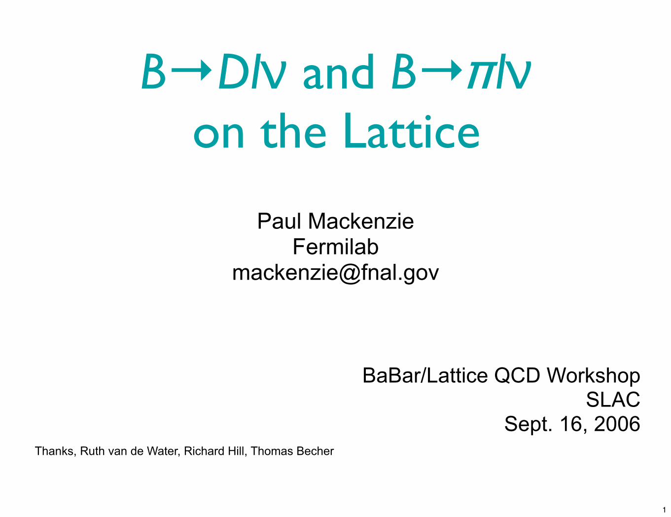
Paul MackenzieFermilab

[email protected]

B→Dlν and B→πlν on the Lattice

BaBar/Lattice QCD WorkshopSLAC

Sept. 16, 2006Thanks, Ruth van de Water, Richard Hill, Thomas Becher

1

mailto:[email protected]

mailto:[email protected]

Paul Mackenzie BaBar/Lattice QCD Workshop, Sept. 16, 2006

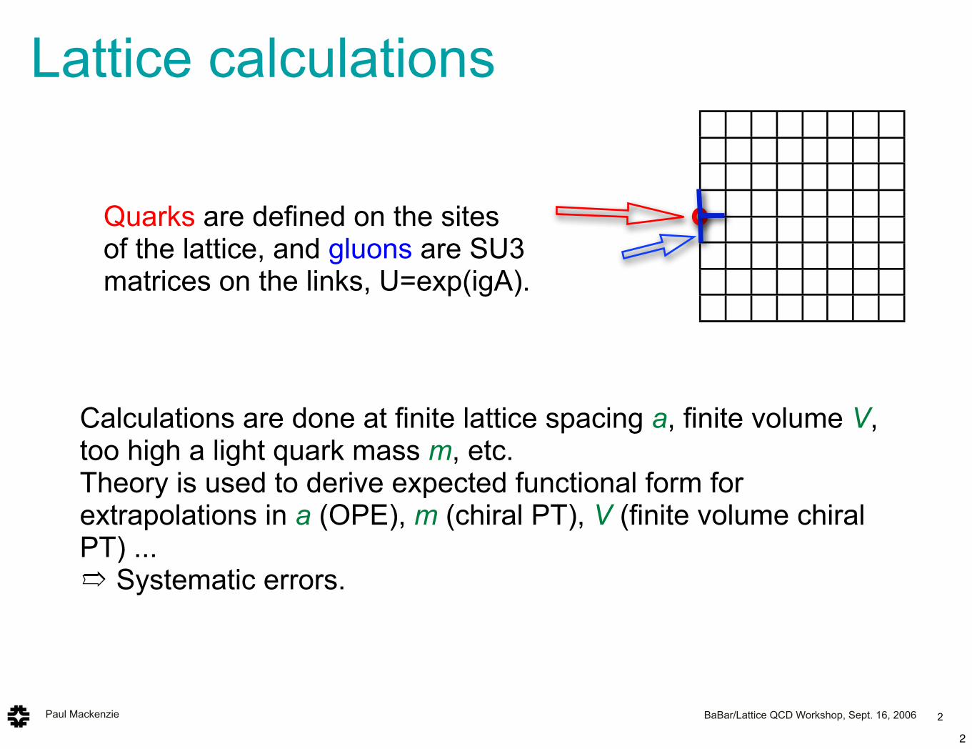
Lattice calculations

2

Quarks are defined on the sitesof the lattice, and gluons are SU3 matrices on the links, U=exp(igA).

Calculations are done at finite lattice spacing a, finite volume V, too high a light quark mass m, etc.Theory is used to derive expected functional form for extrapolations in a (OPE), m (chiral PT), V (finite volume chiral PT) ...➱ Systematic errors.

2

Paul Mackenzie Fermilab Wine and Cheese, July 14, 2006 3

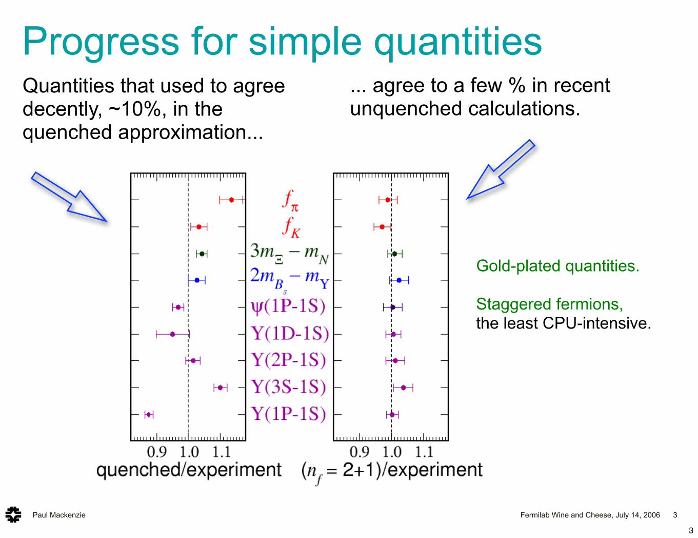
Quantities that used to agree decently, ~10%, in the quenched approximation...

Gold-plated quantities.

Staggered fermions,the least CPU-intensive.

... agree to a few % in recent unquenched calculations.

Progress for simple quantities

3

Paul Mackenzie Fermilab Wine and Cheese, July 14, 2006

Three families of lattice fermions• Staggered (Kogut-Susskind)/naive

• Good chiral behavior (can get to light quark masses). Fermion doubling introduces nonlocal effects which must be theoretically understood. Cheap.

• Wilson/clover

• No fermion doubling but horrible chiral behavior.

• Overlap/domain wall

• Nice chiral behavior at the expense of adding a fifth space-time dimension. Expensive.

4

Staggered fermion unquenched calculations are the cheapest and currently most advanced phenomenologically, (probably a temporary situation).

4

Paul Mackenzie Fermilab Wine and Cheese, July 14, 2006

“Gold-plated quantities” of lattice QCD

5

Quantities that are easiest for theory and experiment to both get right.

Stable particle, one-hadron processes. Especially mesons.

More complicated methods are required for multihadron processes: - unstable particles are messy to interpret, - multihadron final states are different in Euclidean and Minkowski space.

5

Paul Mackenzie Fermilab Wine and Cheese, July 14, 2006 6

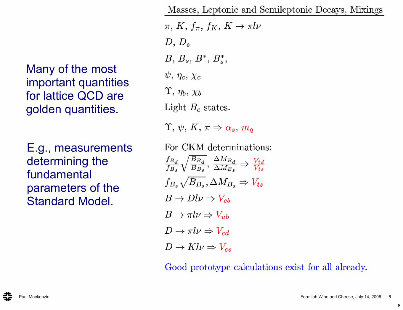
Many of the most important quantities for lattice QCD aregolden quantities.

E.g., measurements determining the fundamental parameters of the Standard Model.

6


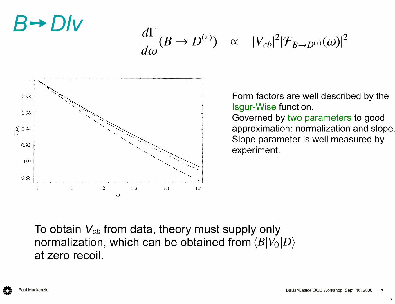
To obtain Vcb from data, theory must supply only normalization, which can be obtained from at zero recoil.

B➙Dlν

7

Constraint on Isgur–Wise function for B ! D semileptonic decays 2025

Figure 1. The function F(!) for " = 0 (full line), 0.02 (short broken) and 0.08 (long broken).

These values of " result from setting g = 0.27 (see main text) and E = 0, 0.5 and 1 GeV,

respectively.

For #$ we then obtain the expression†,

#$ (%, !) = 1

2

!d4p$

(2$)3&(p2$ )&(% " v# · p$ )Tr('+(v)($'+(v#)($ )

= 3

8$2g2

f 20%) 2(!)

"! " 1$

!2 " 1log

#! +

$!2 " 1

%&. (11)

Thus, inequality (7) can be explicitly written as,

)(!) ! F(!) %"1+ !

2+ "

'! " 1$

!2 " 1log

#! +

$!2 " 1

%(&" 12

(12)

" = 3

16$2g2E2

f 20. (13)

The value of E must meet the requirement that contributions to F(!) from higher order

corrections in the perturbative chiral expansion must be small. If, as we expect, the

expansion parameter is gE/(4$f0), a value of E = 0.5 GeV should be appropriate. In

fact, given the relative smallness of g, such choice may be somewhat conservative.

Setting E = 0.5 GeV yields " = 0.275g2. There is a recent determination of g from

D& ! D$ decay data [12], g = 0.27+0.04+0.05"0.02"0.02, which leads to " = 0.020. (Note, however,

that larger values of g are not completely ruled out by current data [12].) The function

F(!) is plotted in figure 1 for several values of ".

The derivative of F(!) at zero recoil is given by

F #(! = 1) = "14

'1+ 8"

3

(. (14)

† #$ vanishes at the zero-recoil point ! = 1 due to the factor in square brackets in (11), a result which holds

true also in the case of many pion emission [13].

Form factors are well described by the Isgur-Wise function.Governed by two parameters to good approximation: normalization and slope.Slope parameter is well measured by experiment.

B! D(!)l! decay

B(B! D(!)l!) " |Vcb|2|FB"D(!)(1)|2Zdw f (!)(w)

where w= vB · vD. Use double ratio (FNAL’99): CDV0B(t)CBV0D(t)

CDV0D(t)CBV0B(t)

! !D|V0|B"!B|V0|D"!D|V0|D"!B|V0|B"

B! Dl!

n f =2+1, FNAL/MILC

0 0.01 0.02 0.03

ml

1

1.1

F(1

)

Nf=2+1 (FNAL/MILC)

Nf=0 (FNAL’99)B!>D

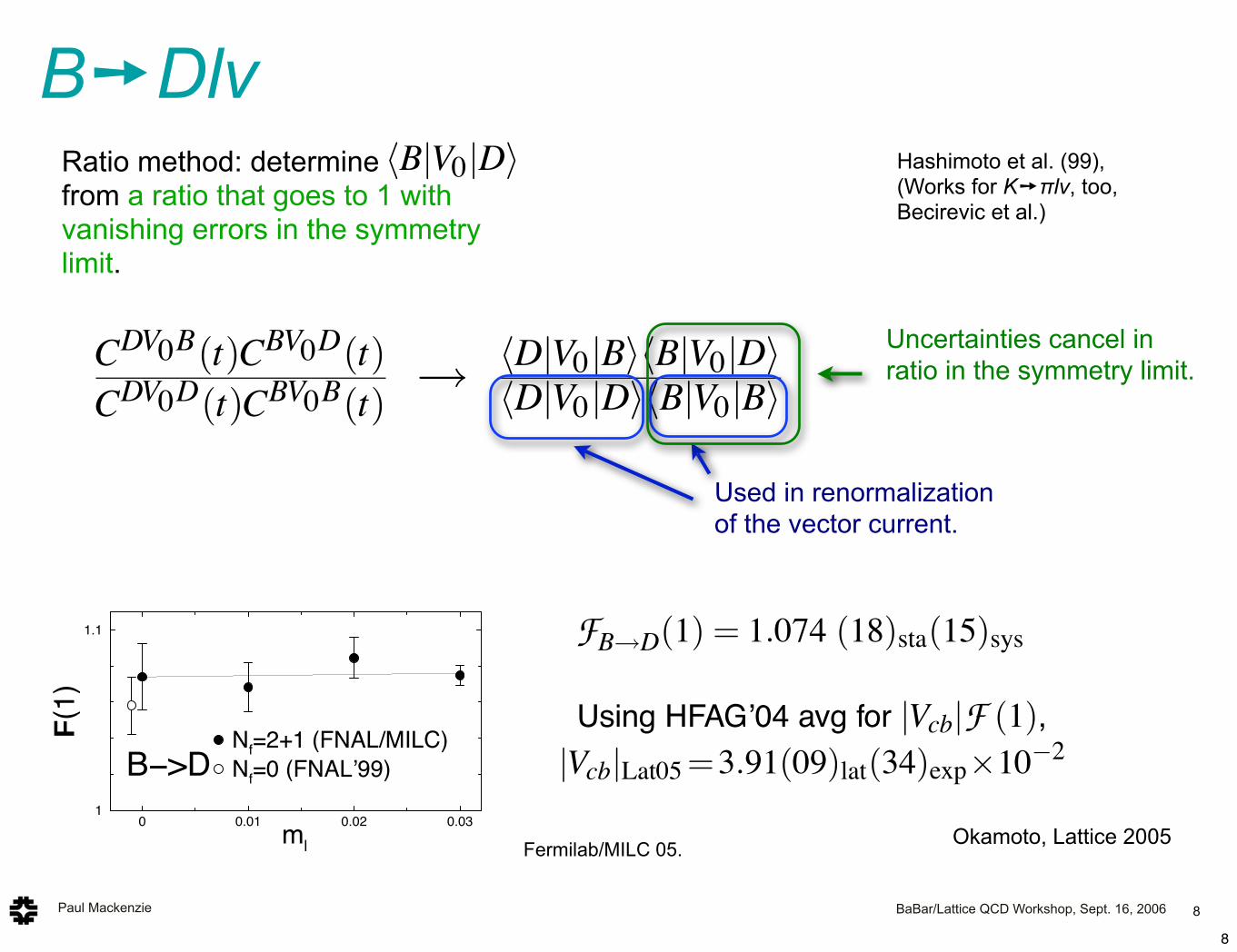
FB"D(1) = 1.074 (18)sta(15)sys

Using HFAG’04 avg for |Vcb|F (1),|Vcb|Lat05=3.91(09)lat(34)exp"10#2

B! D!l!

S#PT calc. completed (Laiho’s talk)

0 0.025 0.05 0.075 0.1 0.125 0.15m_pi^2

0.89

0.9

0.91

0.92

0.93

h_A1

Cusp (in #PT) disappears in S#PT

n f = 2+1 calc. underway (FNAL)=# more precise |Vcb|

4 Workshop on the CKM Unitarity Triangle, IPPP Durham, April 2003

2010-10-20

4

3

2

1

2010-10-20

4

3

2

1

Figure 4. Dispersive bound for f 0 and f + with UKQCD lattice

data. Model-independent QCD bounds with 90%, 70%, 50% and

30% confidence levels are given by the pair of curves. Figure

taken from Ref. [ 7].

in two di!erent methods and equate the results. The two

computational methods are : (1) light cone expansion

which is expressed by the pion light-cone wavefunction

φπ(u) and (2) the dispersion relation which takes the fol-lowing sum of the physical poles

CFv !m2BfB

mb

f +(q2)1

m2B" p2

B

+ higher poles, (5)

where higher poles are suppressed by Borel transformation

with M and approximated by the light-cone expansion re-

sults above a threshold s20.

The theoretical input parameters are the parameters ai’s

of light-cone wavefunctions in the Gegenbauer polynomial

expansion,

φπ = 6u(1 " u)[1 + a2C3/22 (2u " 1) + · · ·], (6)

the B meson decay constant fB, the b quark mass mb, the

threshold s20, and the parameter M for the Borel transfor-

mation.

We here give the new results of Ref. [ 12] as an example.

It is found that the radiative correction is about 10% and

the correction from higher twists ( twist 3) is ! 30%. Theresults for q2 < 14 GeV2 are well fitted by

f +(q2) =F(0)

1 " aq2/m2B+ b(q2/m2

B)2. (7)

Light-cone QCD sum rule results for q2 < 14 GeV2 canalso be fitted by the pole dominance ansatz.

f +(q2) =c

1 " q2/m2B#

(8)

where c $ fB#gBB#π/(2mB#) = 0.414+0.016"0.018 plus systematic

errors.

Fig. 2.1 shows the result by the light-cone QCD sum rule.

It is remarkable that the light-cone QCD sum rule give con-

sistent results with lattice QCD.

3 B% ρlν

Recently, UKQCD collaboration [ 13] and SPQcdR col-

laboration [ 14] started studies of B % ρlν form factors.

Both collaborations use O(a)-improved Wilson action for

the heavy quark and extrapolate the numerical results of

mQ ! mc towards the physical b quark mass. The lattice

spacings are a"1= 2.0 and 2.7 GeV for UKQCD and a"1 =

2.7 and 3.7 GeV for SPQcdR.

UKQCD fits the lattice data for q2 > 14 GeV2 to the fol-lowing form

1

|Vub|2d"

dq2=

G2Fq2[λ(q2)]1/2

192π3m3B

(a + b(q2 " q2max)), .

The fit coe#cients are a = 38+8"5 ± 5 GeV2 and b = 0 ± 2 ±

1, where the first error is statistical and the second is the

extrapolation error for both a and b .

SPQcdR collaboration obtains form factors for q2 > 10GeV2. They find the results which is consistent with the

light-cone QCD sum rule results.

4 B% D(#)lν

One can extract |Vcb| from the B % D(#)lν semileptonicdecay near zero recoil as

d"

dω(B% D(#)) & |Vcb|2|FB%D(#)(ω)|2, (9)

where ω $ v · v' and FB%D(#)lν are the linear combinationsof form factors h±, hA1,2,3 . One important outcome from theheavy quark symmetry is that the form factor FB%D(#)lν isequal to unity at zero recoil up to perturbatively calculable

7


Ratio method: determine from a ratio that goes to 1 with vanishing errors in the symmetry limit.

B! D(!)l! decay



CDV0D(t)CBV0B(t)

! !D|V0|B"!B|V0|D"!D|V0|D"!B|V0|B"

B! Dl!

n f =2+1, FNAL/MILC

0 0.01 0.02 0.03

ml

1

1.1

F(1

)

Nf=2+1 (FNAL/MILC)


FB"D(1) = 1.074 (18)sta(15)sys


B! D!l!


0 0.025 0.05 0.075 0.1 0.125 0.15m_pi^2

0.89

0.9

0.91

0.92

0.93

h_A1



B➙Dlν

8

Hashimoto et al. (99),(Works for K➙πlν, too,Becirevic et al.)

B! D(!)l! decay



CDV0D(t)CBV0B(t)

! !D|V0|B"!B|V0|D"!D|V0|D"!B|V0|B"

B! Dl!

n f =2+1, FNAL/MILC

0 0.01 0.02 0.03

ml

1

1.1

F(1

)

Nf=2+1 (FNAL/MILC)


FB"D(1) = 1.074 (18)sta(15)sys


B! D!l!


0 0.025 0.05 0.075 0.1 0.125 0.15m_pi^2

0.89

0.9

0.91

0.92

0.93h_A1



B! D(!)l! decay



CDV0D(t)CBV0B(t)

! !D|V0|B"!B|V0|D"!D|V0|D"!B|V0|B"

B! Dl!

n f =2+1, FNAL/MILC

0 0.01 0.02 0.03

ml

1

1.1

F(1

)

Nf=2+1 (FNAL/MILC)


FB"D(1) = 1.074 (18)sta(15)sys


B! D!l!


0 0.025 0.05 0.075 0.1 0.125 0.15m_pi^2

0.89

0.9

0.91

0.92

0.93

h_A1



Fermilab/MILC 05.

B! D(!)l! decay



CDV0D(t)CBV0B(t)

! !D|V0|B"!B|V0|D"!D|V0|D"!B|V0|B"

B! Dl!

n f =2+1, FNAL/MILC

0 0.01 0.02 0.03

ml

1

1.1

F(1

)

Nf=2+1 (FNAL/MILC)


FB"D(1) = 1.074 (18)sta(15)sys


B! D!l!


0 0.025 0.05 0.075 0.1 0.125 0.15m_pi^2

0.89

0.9

0.91

0.92

0.93

h_A1



B! D(!)l! decay



CDV0D(t)CBV0B(t)

! !D|V0|B"!B|V0|D"!D|V0|D"!B|V0|B"

B! Dl!

n f =2+1, FNAL/MILC

0 0.01 0.02 0.03

ml

1

1.1

F(1

)

Nf=2+1 (FNAL/MILC)


FB"D(1) = 1.074 (18)sta(15)sys


B! D!l!


0 0.025 0.05 0.075 0.1 0.125 0.15m_pi^2

0.89

0.9

0.91

0.92

0.93

h_A1



Used in renormalization of the vector current.

Uncertainties cancel in ratio in the symmetry limit.

Okamoto, Lattice 2005

8


B➙πlν

9

The players: F+, F

0

!ML(p!)|V µ|MH(p)" = F+(q2)(pµ + p!µ) + F"(q2)(pµ # p!µ)

= F+(q2)

!

pµ + p!µ #m2

H # m2L

q2qµ

"

+ F0(q2)

m2H # m2

L

q2qµ

• What are the measurable quantities ?

• What can we learn ?

2q

0 1 2

+F

0

1

2

3

4

BELLE

2q

0 10 20

+F

0

5

10 BABAR

We also perform model-independent one-dimensional (y) fits where the data in every of the100 q2/m2

! bins were fitted independently. The resulting distribution is shown in Fig.6. Thenormalization f+(0) = 1 is assumed. The visible non-linearity can be observed in Fig.7, wherethe ratio f+(t)/f+(0)/(1 + !+q2/m2

!) is presented. The parabolic curve represents the fit withthe quadratic non-linearity in the form-factor.

q2/m

2!

f(t)/f(0)

Figure 6: The value of f+(t)/f+(0) obtainedin the model-independent fits.

q2/m

2!

Figure 7: The value off+(t)/f+(0)/(1 + !+q2/m2

!). The fit withnon-linear contribution is shown.

This non-linearity can not be explained by a possible scalar contribution (that also resultsin the enhancement of the number of events at large values of q2). The row 4 of the Table1 represents a search for the scalar term with the vector form-factor set to be linear. Theresulting value of fS/f+(0) is compatible with zero.

We also perform a model-independent fit to extract simultaneously f+(t) and fS(t). Theresulting distribution for the value fS(t)/f+(0) is shown in Fig.8. The value of the scalarcontribution is compatible with zero with strong enhancement of the errors at small values oft. This enhancement is explained by the dependence of the scalar contributions (Eq. 2) on theDalitz variables. One can observe that the leading term |S|2 is proportional to t and vanishesat t ! 0.

The last row of the Table 1 represents a fit with both scalar contribution and the quadraticterm in the vector form-factor.

We also do not see any tensor contribution in our data (rows 3 and 5 in the Table 1).

6

!ISTRA

K ! !"# D ! !"# B ! !"#

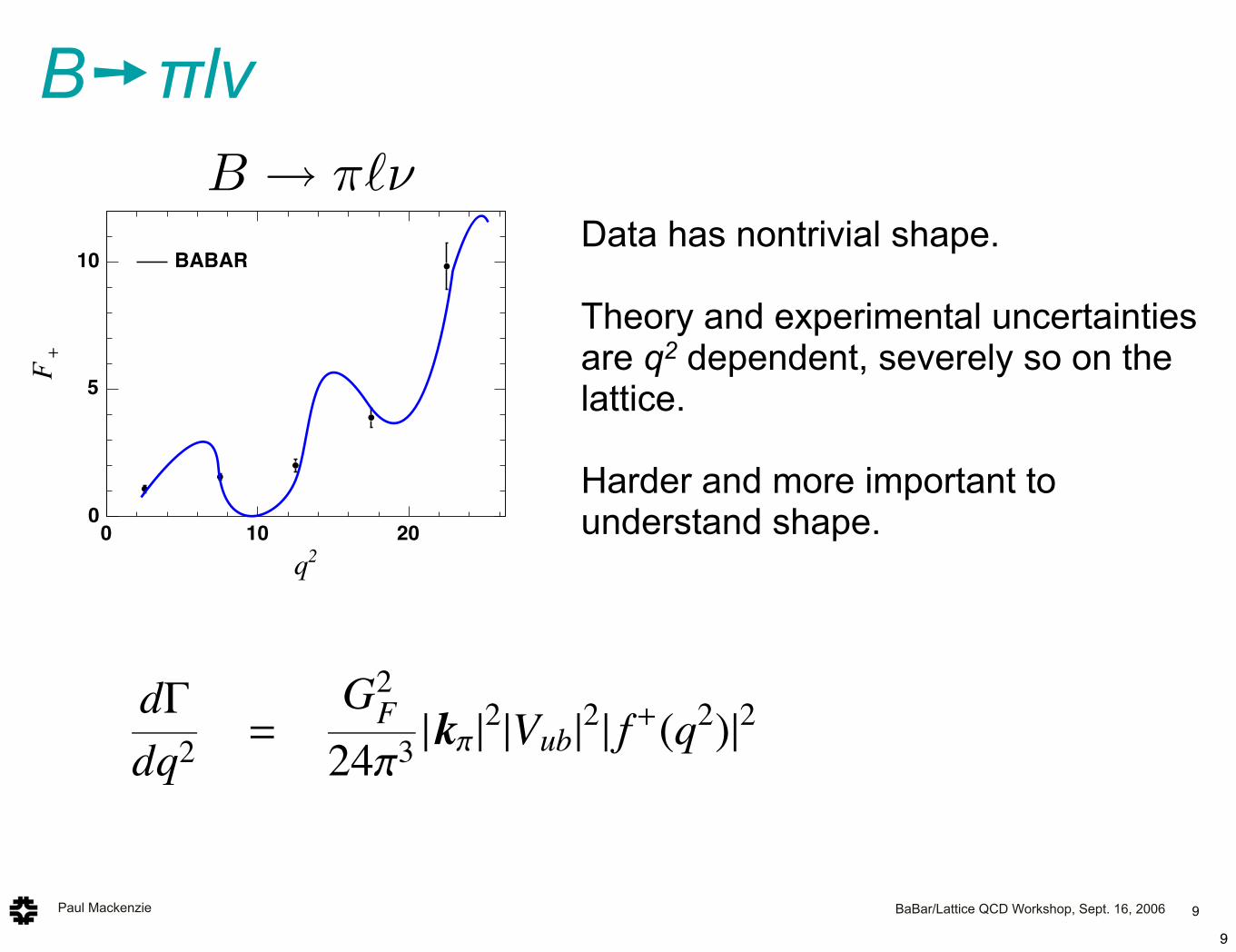
Data has nontrivial shape.

Theory and experimental uncertainties are q2 dependent, severely so on the lattice.

Harder and more important to understand shape.

arX

iv:h

ep-p

h/0

30

92

25

v2

6

Oct

20

03

Workshop on the CKM Unitarity Triangle, IPPP Durham, April 2003

CKM03

Lattice Determination of Semileptonic Form Factors

T. Onogi

Yukawa Institute for Theoretical Physics, Kyoto University, Kyoto, 606-8502, Japan

We report on the Lattice determination of the semileptonic form factors by lattice QCD. Comparison with the light-cone QCD sum rules

are made for B! !l", B! #l" semileptonic decays.

1 Introduction

Computation of the semileptonic form factors for B !!(#)l", B ! D(")l" and B ! K(")l+l# decays is a key to

the determination of the CKM matrix elements |Vub|, |Vcb|and |Vts| . In this report, I review the recent results by lat-

tice QCD methods. I will mainly focus on the semileptonic

decay B ! !l", because lattice calculations in various ap-

proaches are already at hand [ 1, 2, 3, 4, 5] and because

most of the problems which exists in this decay are com-

mon to other processes.

Lattice QCD calculations of B ! !l" form factors su!er

from (1) the error from the large heavy quark mass mQ in

lattice unit, (2) the chiral extrapolations in the light quark

mass mq using the simulation results with relatively large

mass region mq > ms/2, and (3) the limitations from the

accessible kinematic range of q2 from statistical and sys-

tematic errors.

In order to solve the first problem, two di!erent approaches

are made. One is to avoid the large discretization errors of

O(amQ) by computing the form factors with the conven-

tional relativistic quark action for charm quark mass re-

gion, and then extrapolate the results in 1/mQ. The other is

to use HQET e!ective theory with 1/mQ corrections. Since

both approaches have their own advantages and disadvan-

tages, it would be important to have both results and study

whether they give consistent results within quoted errors. I

will present some of the major calculations from these two

approaches and discuss the consistency of the results.

The second problem already gives a source of errors in the

quenched calculations but it would become even more se-

rious in unquenched QCD. Unfortunately, there are still no

results in the unquenched QCD. Since the chiral limit of

the form factors is ill-defined in the quenched QCD, all we

can do with the present lattice data is to discuss the light

quark mass dependence in the intermediate mass regime in

the quenched QCD. However, one may be able to give an

estimate of the low energy coe"cients of the chiral per-

turbation theory based on the present lattice data. I will

briefly review new studies of quenched chiral perturbation

theory (QChPT) and partially quenched chiral perturbation

theory (PQChPT) [ 6] for B ! !l" form factors, which

give a phenomenological estimate on the quenching errors

and chiral extrapolations. These studies will be even more

useful once new calculations in unquenched QCD will be

made.

The third problem arises because in semileptonic decays

large energies are released to the final states so that the lep-

ton pair invariant mass q2 can range from 0 to (mB # m!)2.

However, due to the discretization errors of O(aE) as well

as the statistical errors which grow as $ exp(const % (E #m!)t) where E is the energy of the pion, lattice QCD can

cover only large q2 region. The dispersion relation is a pos-

sible solution to give bounds for smaller q2 region [ 7]. The

light-cone QCD sum rule (LCSR) predicts form factors for

small q2, which is complementary to the lattice results. I

will give a comparison of the recent LCSR results with the

lattice results to see whether they will give consistent re-

sults.

I also review the form factors in other processes. Some

of the recent work on the lattice QCD calculations of the

B ! #l" form factors in relativistic formalism are pre-

sented. Very precise calculations of semileptonic form fac-

tors for B ! D(")l" at zero recoil and the calculations of

the slope of the Isgur Wise function are presented.

2 B! !l"

The exclusive semileptonic decay B ! !l" determines the

CKM matrix element |Vub| through the following formula,

d#

dq2=

G2F

24!3|k!|2|Vub|2| f +(q2)|2, (1)

where the form factor f + is defined as

&!(k!)|q̄$µb|B(pB)' = f +(q2)

!

"

"

"

"

#

(pB + k!)µ #

m2B # m

2!

q2qµ$

%

%

%

%

&

+ f 0(q2)m2B # m

2!

q2qµ, (2)

with q = pB # k! and q2 = m2B + m

2! # 2mBv · k!. The

following parameterization proposed by Burdman et al. [

9


B➙πlν, quenched approximation

10

2 Workshop on the CKM Unitarity Triangle, IPPP Durham, April 2003

8]

!!(k!)|q̄"µb|B(v)" = 2!

f1(v · k!)vµ + f2(v · k!)kµ!

v · k!

"

, (3)

is also useful for discussing the heavy quark symmetry and

the chiral symmetry of the form factors in a transparent

way.

2.1 Lattice results

Lattice calculation is possible only in limited situations.

Spatial momenta must be much smaller than the cuto!, i.e.

|#pB|, |#k!| < 1 GeV. This means v·k! # E! < 1 GeV or equiv-alently q2 > 18 GeV2. Another limitation is that due tothe slowing down, simulations with very small light quark

masses are di"cult so that usual mass range for the light

quark masses in practical simulations is ms/3 $ mq $ ms

or m! = 0.4 % 0.8 GeV. Therefore in order to obtain phys-ical results chiral extrapolations in the light quark masses

are necessary.

So far all the lattice calculations of the form factors are

done only in quenched approximation. APE collaboration

[ 1] and UKQCD collaboration computed B & !l$ formfactors for a fine lattice with the inverse lattice spacing

a'1 % 2.7 GeV. They used relativistic formalism for the

heavy quark and extrapolated the results of heavy-lightme-

son around charm quark masses to the bottom quark mass.

Fermilab collaboration [ 3] used the Fermilab formalism

for the heavy quark and computed the form factors on three

lattices with a'1 = 1.2 % 2.6 GeV . JLQCD collaboration[ 4] computed the form factors using NRQCD formalism

for the heavy quark on a a'1 = 1.64 GeV. NRQCD col-

laboration [ 5] also used NRQCD formalism for the heavy

quark and an improved light quark action (D234 action)

on a anisotropic lattice with a'1 = 1.2 GeV (spatial), 3.3GeV (temporal). In all of these calculations the light pseu-

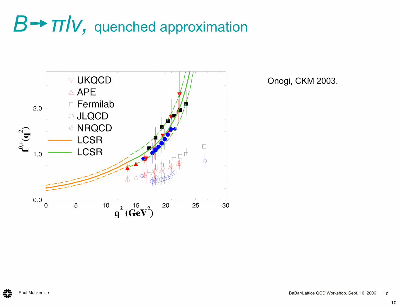
doscalar meson masses are 0.4 % 0.8 GeV. Fig. 1 showsthe result by di!erent lattice groups, f +(q2) agrees within

systematic errorswhile f 0(q2) shows deviations among dif-

ferent methods.

The reason for the discrepancies in f 0 can be attributed to

the systematic error in the chiral extrapolation and heavy

quark mass extrapolation (interpolation) error. In the fol-

lowing, we examine these errors in more detail. Light

quark mass mq dependence of form factors with fixed spa-

tial momenta ap = 2!16(1, 0, 0) is shown in Fig. 2. In con-

trast to the JLQCD data, Fermilab data shows a significant

increase towards the chiral limit. Large di!erence in Fer-

milab results and JLQCD results for f 0 in the chiral limit

arises from di!erent mq dependence, but the raw data for

similar quark masses are not so di!erent. Shigemitsu et al.

studied the mass dependence of f1 + f2 and find similar be-

havior as JLQCD. Further studies to clarify the light quark

mass dependence are required.

0 5 10 15 20 25 30

q2 (GeV

2)

0.0

1.0

2.0

f0,+(q

2)

UKQCD

APE

Fermilab

JLQCD

NRQCD

LCSR

LCSR

Figure 1. B& !l$ form factors by di!erent lattice groups.

Fig. 3 shows 1/MB dependence of form factors #0,+ #(mB f

0,+ at v · k! = 0.845 GeV for APE and JLQCD col-laboration data. It is found that the di!erence of APE

(UKQCD) vs JLQCD (NRQCD) for f 0 arises from the ex-

trapolation in 1/M. Linear extrapolation in 1/M is consis-

tent, while the quadratic extrapolation gives higher value.

The quadratic extrapolation 1/M is chosen for APE’s result,

since higher value gives better agreement with the soft pion

theorem. Simulations with static heavy quark may resolve

the problem.

The error of the form factors in the present calculations is

around 20%. Some of the major errors are the quenching

error, chiral extrapolation error statistical error in all cal-

culations. In addition, a large discretization error appears

in JLQCD results and a large 1/M extrapolation error is

contained in APE and UKQCD results.

There are several proposals to improve the form factor de-

termination. The quenching error can be resolved only

by performing the unquenched calculations. Recently,

JLQCD and UKQCD collaborations has accumulated n f =

2 unquenched lattice configurations with O(a)-improved

Wilson fermions and n f = 2+1 unquenched configurations

with improved staggered fermions have been produced by

the MILC collaboration. These unquenched QCD data

should be applied to form factor calculations.

In order to reduce the chiral extrapolation error, simulation

with even smaller light quark masses are necessary. For

Wilson type fermions, simulations with m! < 0.4 GeV willbe very slow and also appearance of exceptional configura-

tion may prevent the simulation for very light quark mass

range. On the other hand, MILC collaboration is now car-

rying out simulations with m! = 0.3' 0.5 GeV, which cor-responds tomq = 1/5ms'1/2ms [ 9]. Since n f = 2+1 sim-

ulations are performed by taking the square root or quar-

Onogi, CKM 2003.

10


B➙πlν, unquenched

11

27

0 5 10 15 20 25

q2 [GeV

2]

0.0

1.0

2.0

3.0

UKQCD (1999)

Abada et al. (2000)

El-Khadra et al. (2001)

JLQCD (2001)

0 5 10 15 20 25

q2 [GeV

2]

0.0

1.0

2.0

3.0

Fermilab (2004)

HPQCD (2004)

Nf = 0

Nf = 2+1

0 5 10 15 20 25

q2 [GeV

2]

0

0.5

1

1.5

2

2.5N

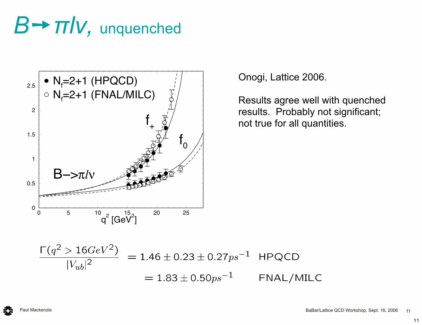
f=2+1 (HPQCD)

Nf=2+1 (FNAL/MILC)

B!>!l"

f+

f0

Onogi, Lattice 2006.

Results agree well with quenched results. Probably not significant; not true for all quantities.

27

0 5 10 15 20 25

q2 [GeV

2]

0.0

1.0

2.0

3.0

UKQCD (1999)

Abada et al. (2000)


JLQCD (2001)

0 5 10 15 20 25

q2 [GeV

2]

0.0

1.0

2.0

3.0

Fermilab (2004)

HPQCD (2004)

Nf = 0

Nf = 2+1

0 5 10 15 20 25

q2 [GeV

2]

0

0.5

1

1.5

2

2.5N

f=2+1 (HPQCD)

Nf=2+1 (FNAL/MILC)

B!>!l"

f+

f0

11


B➙πlν, finite range of q2

12

27

0 5 10 15 20 25

q2 [GeV

2]

0.0

1.0

2.0

3.0

UKQCD (1999)

Abada et al. (2000)


JLQCD (2001)

0 5 10 15 20 25

q2 [GeV

2]

0.0

1.0

2.0

3.0

Fermilab (2004)

HPQCD (2004)

Nf = 0

Nf = 2+1

0 5 10 15 20 25

q2 [GeV

2]

0

0.5

1

1.5

2

2.5N

f=2+1 (HPQCD)

Nf=2+1 (FNAL/MILC)

B!>!l"

f+

f0

The players: F+, F

0

!ML(p!)|V µ|MH(p)" = F+(q2)(pµ + p!µ) + F"(q2)(pµ # p!µ)

= F+(q2)

!

pµ + p!µ #m2

H # m2L

q2qµ

"

+ F0(q2)

m2H # m2

L

q2qµ

• What are the measurable quantities ?

• What can we learn ?

2q

0 1 2

+F

0

1

2

3

4

BELLE

2q

0 10 20

+F

0

5

10 BABAR

We also perform model-independent one-dimensional (y) fits where the data in every of the100 q2/m2

! bins were fitted independently. The resulting distribution is shown in Fig.6. Thenormalization f+(0) = 1 is assumed. The visible non-linearity can be observed in Fig.7, wherethe ratio f+(t)/f+(0)/(1 + !+q2/m2

!) is presented. The parabolic curve represents the fit withthe quadratic non-linearity in the form-factor.

q2/m

2!

f(t)/f(0)

Figure 6: The value of f+(t)/f+(0) obtainedin the model-independent fits.

q2/m

2!

Figure 7: The value off+(t)/f+(0)/(1 + !+q2/m2

!). The fit withnon-linear contribution is shown.

This non-linearity can not be explained by a possible scalar contribution (that also resultsin the enhancement of the number of events at large values of q2). The row 4 of the Table1 represents a search for the scalar term with the vector form-factor set to be linear. Theresulting value of fS/f+(0) is compatible with zero.

We also perform a model-independent fit to extract simultaneously f+(t) and fS(t). Theresulting distribution for the value fS(t)/f+(0) is shown in Fig.8. The value of the scalarcontribution is compatible with zero with strong enhancement of the errors at small values oft. This enhancement is explained by the dependence of the scalar contributions (Eq. 2) on theDalitz variables. One can observe that the leading term |S|2 is proportional to t and vanishesat t ! 0.

The last row of the Table 1 represents a fit with both scalar contribution and the quadraticterm in the vector form-factor.

We also do not see any tensor contribution in our data (rows 3 and 5 in the Table 1).

6

!ISTRA

K ! !"# D ! !"# B ! !"#

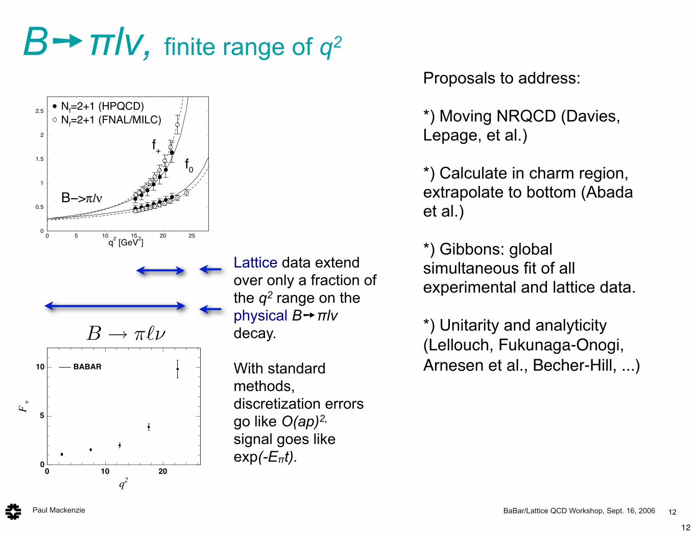
Lattice data extend over only a fraction of the q2 range on the physical B➙πlν decay.

With standard methods, discretization errors go like O(ap)2,

signal goes like exp(-Eπt).

Proposals to address:

*) Moving NRQCD (Davies, Lepage, et al.)

*) Calculate in charm region, extrapolate to bottom (Abada et al.)

*) Gibbons: global simultaneous fit of all experimental and lattice data.

*) Unitarity and analyticity (Lellouch, Fukunaga-Onogi, Arnesen et al., Becher-Hill, ...)

12


B➙πlν, unitarity fits

13

2q

0 10 20

+F

0

5

10 BABAR

B!!

• Experiment has yet to observe more than a normalization and a slope

• What is the significance of this slope?

-z

-0.2 0 0.2

+ F!

P

-1

0

1

2

3

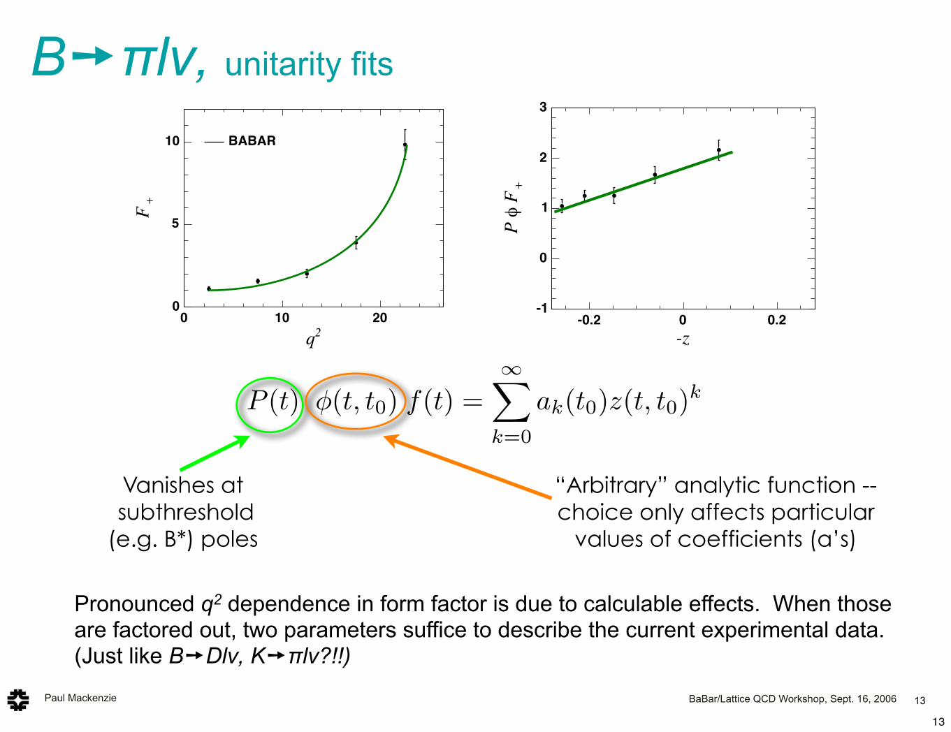
Pronounced q2 dependence in form factor is due to calculable effects. When those are factored out, two parameters suffice to describe the current experimental data.(Just like B➙Dlν, K➙πlν?!!)

“Arbitrary” analytic function -- choice only affects particular

values of coefficients (a’s)

Vanishes at subthreshold (e.g. B*) poles

P (t) !(t, t0) f(t) =!!

k=0

ak(t0)z(t, t0)k

13



14

-0.2 -0.1 0 0.1 0.2z(t)

0

0.05

0.1

P(t

)!(t

,t0)f

(t)

P(t)!(t,t0)f

0(t)

P(t)!(t,t0)f

+(t)

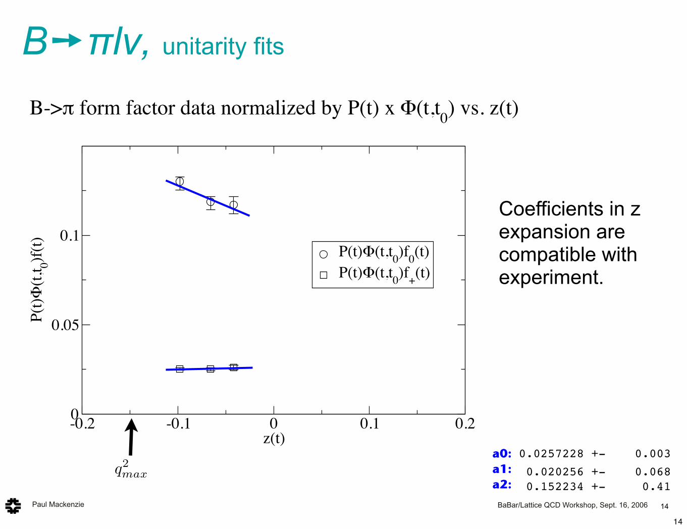
B->" form factor data normalized by P(t) x !(t,t0) vs. z(t)

q2

max

Coefficients in z expansion are compatible with experiment.

0.0257228 +- 0.003 0.020256 +- 0.068

0.152234 +- 0.41

a0:a1:a2:

14



15

0 5 10 15 20

q2(GeV

2)

0

0.5

1

1.5

2

2.5

3

3.5

f 0(q

2)

and

f+(q

2)

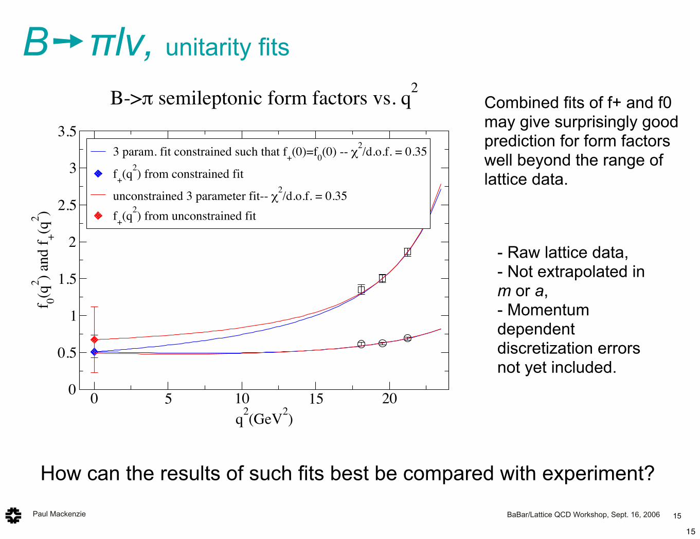
3 param. fit constrained such that f+(0)=f

0(0) -- !

2/d.o.f. = 0.35

f+(q

2) from constrained fit

unconstrained 3 parameter fit-- !2/d.o.f. = 0.35

f+(q

2) from unconstrained fit

B->" semileptonic form factors vs. q2

- Raw lattice data,- Not extrapolated in m or a,- Momentum dependent discretization errors not yet included.

Combined fits of f+ and f0 may give surprisingly good prediction for form factors well beyond the range of lattice data.

How can the results of such fits best be compared with experiment?

15


Not covered, but interesting

• B➙ρlν, B➙ωlν, etc.

• Honest methods for treating unstable particles on the lattice exist (Lüscher,...) but they are much more demanding.

• B➙Klν, non-Standard Model effects

• Lattice calculation are no more difficult as long as effective operators are local.

16

16


Summary and to-do list

• For lattice theorists: how well do lattice methods agree?

• staggered vs. clover vs. overlap, etc.

• Will Moving NRQCD allow calculation of the form factors for B➙πlν in the whole decay region?

• For theorists and experimentalists: how should lattice data be reported; how should lattice and experiment be compared?

• Raw lattice data in large global fit (Gibbons)

• Normalization and slope in the z expansion

• Form factor and slope at several fiducial points (Becher and Hill)

• All of the above

17

17

Documents

on the Lattice - slac.stanford.edu · Thanks, Ruth van de Water, Richard Hill, Thomas Becher 1. Paul Mackenzie BaBar/Lattice QCD Workshop, Sept. 16, 2006 Lattice calculations 2 Quarks