On the Linkages between the Tropospheric Isentropic Slope

On the Linkages between the Tropospheric Isentropic Slope and Eddy Fluxesof Heat during Northern Hemisphere Winter

DAVID W. J. THOMPSON AND THOMAS BIRNER

Department of Atmospheric Science, Colorado State University, Fort Collins, Colorado

(Manuscript received 13 July 2011, in final form 12 December 2011)

ABSTRACT

Previous studies have demonstrated the key role of baroclinicity and thus the isentropic slope in de-

termining the climatological-mean distribution of the tropospheric eddy fluxes of heat. Here the authors

examine the role of variability in the isentropic slope in driving variations in the tropospheric eddy fluxes of

heat about their long-term mean during Northern Hemisphere winter.

On month-to-month time scales, the lower-tropospheric isentropic slope and eddy fluxes of heat are not

significantly correlated when all eddies are included in the analysis. But the isentropic slope and heat fluxes

are closely linked when the data are filtered to isolate the fluxes due to synoptic (,10 days) and low-frequency

(.10 days) time scale waves. Anomalously steep isentropic slopes are characterized by anomalously poleward

heat fluxes by synoptic eddies but anomalously equatorward heat fluxes by low-frequency eddies. Lag re-

gressions based on daily data reveal that 1) variations in the isentropic slope precede by several days variations

in the heat fluxes by synoptic eddies and 2) variations in the heat fluxes due to both synoptic and low-frequency

eddies precede by several days similarly signed variations in the momentum flux at the tropopause level.

The results suggest that seemingly modest changes in the tropospheric isentropic slope drive significant

changes in the synoptic eddy heat fluxes and thus in the generation of baroclinic wave activity in the lower

troposphere. The linkages have implications for understanding the extratropical tropospheric eddy response

to a range of processes, including anthropogenic climate change, stratospheric variability, and extratropical

sea surface temperature anomalies.

1. Context

Feedbacks between the mean flow and the wave fluxes

of heat and momentum play a fundamental role in the

general circulation of the extratropical troposphere (e.g.,

Holton 2004, ch. 10; Vallis 2006, ch. 12). For example,

wave activity is predominantly generated near the sur-

face in regions of large isentropic slopes (Fig. 1a; e.g.,

Stone 1978). Much of the wave activity generated in

the lower troposphere propagates vertically and is thus

associated with poleward fluxes of heat in the free

troposphere. If the wave activity dissipates in the upper

troposphere at roughly the same latitude range as the

wave source (Fig. 1b), then the westward torque aloft

drives a residual (mass) circulation with rising motion

equatorward of the wave source and sinking motion

poleward of the wave source. The anomalous vertical

motion acts to reduce the lower-tropospheric isentropic

slope that generated the wave activity in the first place.

As such, the residual circulation induced by the wave

breaking aloft acts as a negative feedback that attenu-

ates lower tropospheric baroclinicity.

A somewhat different relationship holds between the

lower-tropospheric isentropic slope and the wave fluxes

of momentum. For example, assume that a component

of the upper-tropospheric wave activity in Fig. 1b prop-

agates equatorward near the tropopause. The equator-

ward wave propagation is associated with poleward

momentum fluxes that converge at the source latitude

(Fig. 1c). Viewed in isolation, the momentum fluxes

induce a residual circulation that acts to reinforce rather

than damp the lower-tropospheric isentropic slope in

the wave source region (Fig. 1c). Hence, the residual

circulation induced by the momentum flux convergence

aloft acts as a positive feedback that increases lower-

tropospheric baroclinicity.

In the climatological mean, the wave driving due to

the vertical convergence of the wave flux (i.e., the ver-

tical convergence of the heat flux) is larger than that due

Corresponding author address: David W. J. Thompson, Colorado

State University, Department of Atmospheric Science, Campus

Delivery 1371, Fort Collins, CO 80523.

E-mail: [email protected]

JUNE 2012 T H O M P S O N A N D B I R N E R 1811

DOI: 10.1175/JAS-D-11-0187.1

� 2012 American Meteorological Society

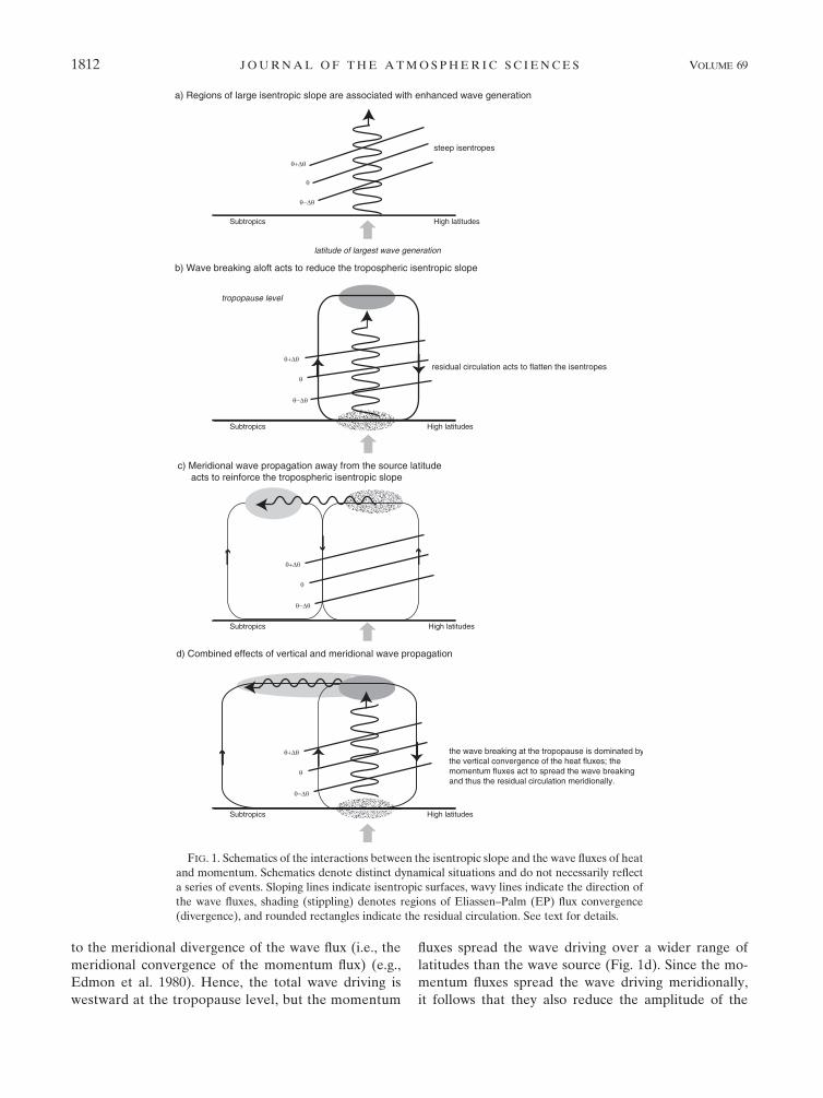
to the meridional divergence of the wave flux (i.e., the

meridional convergence of the momentum flux) (e.g.,

Edmon et al. 1980). Hence, the total wave driving is

westward at the tropopause level, but the momentum

fluxes spread the wave driving over a wider range of

latitudes than the wave source (Fig. 1d). Since the mo-

mentum fluxes spread the wave driving meridionally,

it follows that they also reduce the amplitude of the

FIG. 1. Schematics of the interactions between the isentropic slope and the wave fluxes of heat

and momentum. Schematics denote distinct dynamical situations and do not necessarily reflect

a series of events. Sloping lines indicate isentropic surfaces, wavy lines indicate the direction of

the wave fluxes, shading (stippling) denotes regions of Eliassen–Palm (EP) flux convergence

(divergence), and rounded rectangles indicate the residual circulation. See text for details.

1812 J O U R N A L O F T H E A T M O S P H E R I C S C I E N C E S VOLUME 69

compensating poleward mass flux at the latitude of the

wave source. As a result, the wave-driven residual cir-

culation attenuates the lower-tropospheric isentropic

slope, but not as much as it would if all the wave-breaking

was concentrated at the latitude of the wave source (e.g.,

Robinson 2000, 2006).

The relationships among the isentropic slope, tropo-

spheric wave generation, and tropospheric wave dissi-

pation reviewed schematically in Fig. 1 are known to

play a key role in determining the climatological-mean

extratropical circulation. The largest eddy fluxes of heat

are roughly collocated with the regions of largest lower-

tropospheric baroclinicity (Kushner and Held 1998); the

largest momentum fluxes are closely collocated with the

extratropical storm tracks (e.g., Lau et al. 1978; Lim and

Wallace 1991). However, the role of the isentropic slope

in driving variability in the extratropical wave fluxes of

heat and momentum remains unclear. The amplitude of

such a feedback is important, since the sensitivity of the

eddies to variations in the isentropic slope is theorized to

play a potentially key role in driving the following: 1) the

internal feedbacks that give rise to the annular modes

(e.g., Robinson 2000, 2006; Lorenz and Hartmann 2001,

2003); 2) the storm track response to extratropical sea

surface temperature anomalies (e.g., Kushnir et al. 2002,

and references therein; Brawshay et al. 2008); 3) the ex-

tratropical tropospheric response to stratospheric var-

iability (e.g., Song and Robinson 2004); and 4) the storm

track response to increasing greenhouse gases (e.g.,

Kushner et al. 2001; Yin 2005; Frierson 2006; Lu et al.

2008, 2010; Chen et al. 2010; O’Gorman 2010; Scaife

et al. 2012; Butler et al. 2011).

The primary purpose of this study is to quantify the

observed relationships between variability in the isen-

tropic slope and the eddy fluxes of heat and momentum

in the Northern Hemisphere (NH) tropospheric circula-

tion. The results imply that low-frequency time scale ed-

dies primarily force anomalies in the baroclinicity, whereas

synoptic time scale eddies respond to anomalies in the

baroclinicity. The dataset is discussed in section 2; results

are presented in section 3; implications of the results for

climate variability are discussed in section 4.

2. Data and analysis

The primary dataset is 4-times-daily values of the in-

terim European Centre for Medium-Range Weather

Forecasts (ECMWF) Re-Analysis (ERA-Interim) data

from 1 January 1989 to 31 December 2009 (see ECMWF

Newsletter, No. 110; Dee et al. 2011). The reanalyses

products are available on a 1.58 3 1.58 mesh, and are

daily and zonally averaged before computing regres-

sions and correlations. The zonal mean fluxes of heat

and momentum are defined as [y*T*] and [u*y*], re-

spectively, where brackets denote the zonal mean and

stars denote the departure from the zonal mean. The

fluxes are calculated at 4-times-daily resolution before

being daily averaged. Anomalies are defined throughout

the study as departures from the long-term mean sea-

sonal cycle. All results are calculated for the Northern

Hemisphere, for anomalies, and for the winter months

of December–February (DJF).

The wave fluxes of heat due to synoptic and low-

frequency time scale eddies were estimated by decom-

posing the fluxes as follows:

[y*T*] 5 [ys*Ts

*] 1 [yl*Tl

*] 1 cross terms,

where the synoptic time scale (denoted by subscript s) is

defined as less than 10 days and the low-frequency time

scale (denoted by subscript l) is defined as longer than

10 days. The time filtering was done using an eighth-

order Butterworth filter with a cutoff frequency of

10 days. A similar procedure was applied to the eddy

fluxes of momentum.

Note that the synoptic eddies exhibit variability on

time scales longer than 10 days, even though the wind

and temperature time series have both been 10-day

high-pass filtered. As noted in Lorenz and Hartmann

(2001), the redness of the synoptic eddy fluxes is consis-

tent with a positive feedback between the synoptic eddy

fluxes and the mean flow. The cross terms are generally

small and are not considered here.

We exploit the ERA-Interim products in both isen-

tropic and pressure coordinates. To orient the reader to

our use of both coordinate systems, Fig. 2 shows the

DJF-mean, zonal-mean Northern Hemisphere circula-

tion as a function of (left) latitude and pressure and

(right) latitude and potential temperature. In both

panels, the height of the tropopause (thick line) is ap-

proximated as the level where potential vorticity is equal

to 2 potential vorticity units (PVU; 1 PVU 5 1026 K

kg21 m2 s21). Key surfaces used in the results section

include 1) the 285-K isentrope, which extends from the

surface in the subtropics near 358, spans the lower

troposphere at mid- to high latitudes, and reaches the

500-hPa level at polar latitudes; 2) the 700-hPa level,

which lies near the top of the atmospheric boundary

layer; and 3) the 300-hPa level, which lies in the upper-

troposphere/lower-stratosphere region.

Variability in the strength of the extratropical strato-

spheric vortex is defined as the leading principal com-

ponent time series of the zonal-mean 10-hPa geopotential

height field. The index is generated according to Baldwin

and Thompson (2009) and is referred to as the northern

annular mode index at 10 hPa (NAM10). By definition,


positive values of the NAM10 index denote a stronger

than normal stratospheric vortex, and vice versa. [Note

that the results in Fig. 9 are based on inverted values of

the NAM10 index (i.e., the index is multiplied by 21) so

that the regression coefficients correspond to weakenings

of the stratospheric circumpolar zonal flow.]

Statistical significance of key results is assessed using

a one-tailed test of the t statistic. The effective degrees of

freedom are estimated using the autocorrelation charac-

teristics of the respective time series. By definition, stan-

dardized time series have a mean of zero and standard

deviation of one.

3. Observed linkages between variability in thetropospheric isentropic slope and eddy fluxesof heat and momentum

The meridional slope of extratropical isentropic sur-

faces provides a succinct measure of the tendency of the

atmosphere to generate wave activity (e.g., Stone 1978;

Stone and Nemet 1996). The isentropic slope is—by

definition—given as (minus) the ratio of the meridional

and vertical gradients in potential temperature. In-

creases in the amplitude of the meridional potential

temperature gradient (i.e., the baroclinicity) and de-

creases in the vertical potential temperature gradient

(i.e., the static stability) both increase the isentropic

slope and thus the instability of the flow to the genera-

tion of baroclinic waves. The meridional slope of the

isentropes is related to the available potential energy of

the general circulation (e.g., Lorenz 1955) and is closely

related to the Eady growth rate (the Eady growth rate is

proportional to the meridional temperature gradient

divided by the buoyancy frequency; Lindzen and Farrell

1980).

The isentropic slope is calculated here as the meridi-

onal gradient in pressure along isentropic surfaces; that

is,

2(›u/›y)p

(›u/›p)y

5›p

›y

� �u

[ sp,

where u denotes potential temperature, p denotes

pressure, and the subscripts denote the variable that is

held constant in the derivative. The resulting slope sp is

in units of hectopascals per kilometer and is converted

to meters (vertical) per kilometer (horizontal) using the

hypsometric equation assuming a scale height of 7 km

and a reference pressure of 1000 hPa.

The isentropic slope affects wavelike variability not

only through its relation to baroclinic instability, but also

through its projection onto the meridional gradient of

potential vorticity (PV) along isentropic surfaces. For

example, the meridional gradient in PV along isentropic

surfaces can be written as

›P

›y

� �u

5›P

›y

� �p

1 sp

›P

›p’ P

b

f2

›sp

›p

� �, (1)

where P denotes the zonal-mean potential vorticity.

Here we have neglected the relative vorticity contri-

bution to zonal-mean PV—that is, we have made the

‘‘planetary approximation’’ so that P ’ 2gf (›u/›p).

As evidenced in (1), the vertical derivative of the isen-

tropic slope is directly related to the meridional PV

gradient and thus is a central component of the index

of refraction for wave propagation.

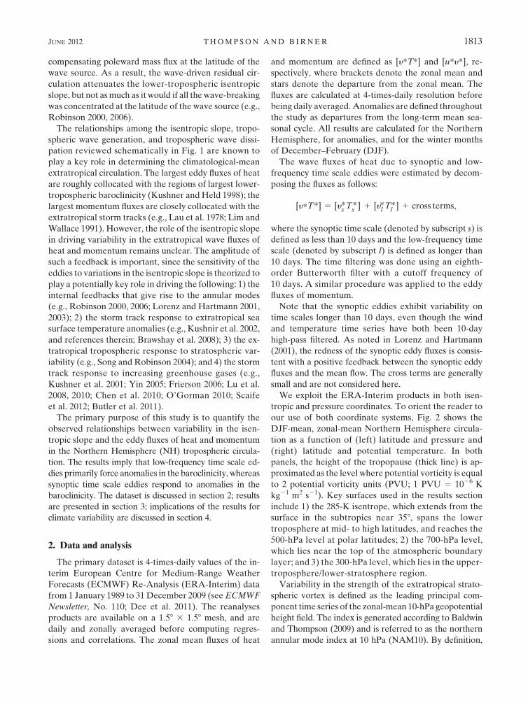
Figure 3a explores the linkages between the zonal-

mean eddy fluxes of heat at 700 hPa ([y*T*]700hPa) and

the zonal-mean isentropic slope at 285 K (s285K; the 285-K

FIG. 2. NH DJF-mean, zonal-mean circulation in (left) pressure and (right) isentropic coordinates. Dashed lines

indicate (left) isentropic surfaces and (right) pressure surfaces, thin solid lines indicate the zonal wind, and the thick

solid lines indicate the 2-PVU isoline and thus approximate the height of the dynamical tropopause. The isentropic

levels in the right panel correspond to the isentropic levels available in the ERA-Interim dataset.


isentrope spans the lower troposphere at mid- to high

latitudes; see Fig. 2). The results are calculated for monthly

mean anomaly data and for the winter season months of

DJF. The solid line shows unfiltered values of [y*T*]700hPa

regressed onto standardized values of s285K as a function

of latitude (e.g., the coefficient at 558N corresponds to the

regression of [y*T*]700hPa at 558N onto standardized values

of s285K at 558N). The dashed and dot-dashed lines show

corresponding results calculated for the synoptic and low-

frequency eddy heat fluxes, respectively. Results are not

shown for latitude bands where the 285-K surface in-

tersects the earth’s surface (equatorward of about 358N).

The unfiltered eddy heat fluxes are negatively corre-

lated with the isentropic slope at all latitudes, but the

regression coefficients are weak and are not statistically

significant (the 95% significance bounds are given by the

light shading and are described in the figure caption).

Interestingly, the synoptic (dashed) and low-frequency

(dot-dashed) eddy heat fluxes exhibit highly significant

but opposite-signed relationships with the slope. Anoma-

lously steep isentropic slopes are associated with 1) anom-

alously poleward heat fluxes by synoptic eddies but 2)

anomalously equatorward heat fluxes by low-frequency

eddies. That is, the anomalous synoptic eddy heat fluxes

are anomalously downgradient (down the anomalous

meridional temperature gradient) whereas the anoma-

lous low-frequency eddy heat fluxes are countergradient

(up the anomalous meridional temperature gradient).

The eddy fluxes of heat at 700 hPa are a proxy for

the eddy fluxes of PV and thus the generation of wave

FIG. 3. (a) Regression of monthly mean values of the eddy heat flux at 700 hPa onto stan-

dardized values of the isentropic slope at 285 K. The solid line denotes results for unfiltered data,

the dashed line is for the eddy fluxes of heat calculated from wind and temperature data that have

been 10-day high-pass filtered (i.e., the synoptic eddy fluxes), and the dash-dotted line is for data

that have been 10-day low-pass filtered (i.e., the low-frequency eddy fluxes). Units are K m s21

per standard deviation fluctuation in the slope. (b) Regression of monthly mean values of the

synoptic eddy heat fluxes at 700 hPa onto standardized values of the meridional temperature

gradient at 700 hPa. The results are multiplied by 21 and are equivalent to the eddy diffusivity on

monthly time scales (see text for details). All regressions are calculated as a function of latitude

(e.g., the coefficients at 558N denote the regression of the heat flux at 558N onto the slope or

temperature gradient at 558N). Results are based on anomalies for the NH winter months (DJF).

Shading in (a) above (below) the zero line denotes the 95% significance bounds for the synoptic

(low frequency) eddy fluxes based on 1 degree of freedom per winter month (significant results

exceed the shaded regions).


activity at the lower boundary (i.e., the divergence of the

eddy heat flux at the surface; Held and Schneider 1999).

Thus, the in-phase relationship between anomalies in

the slope and the synoptic eddy heat flux is consistent

with theories of baroclinic instability (i.e., anomalously

steep isentropes lead to increased baroclinic wave gen-

eration and thus anomalously poleward eddy heat fluxes,

and vice versa). The diffusive nature of baroclinic eddies

has been clearly established in the context of the long-

term-mean climatology (e.g., Kushner and Held 1998)

but to our knowledge has not been quantified in the

context of month-to-month variability in the isentropic

slope. The out-of-phase relationship between anoma-

lies in the slope and the low-frequency eddy heat flux is

consistent with forcing of zonal-mean temperature by

the eddy heat flux convergence (i.e., anomalously pole-

ward eddy heat fluxes act to flatten the isentropic slope,

and vice versa).

The month-to-month ‘‘synoptic eddy diffusivity’’ can

be estimated by regressing the (anomalous) zonal mean

synoptic eddy heat flux at 700 hPa [y*T*]synoptic700hPa onto the

(anomalous) meridional temperature gradient at 700 hPa

(›/›y)T700hPa. That is,

[y*T*]synoptic700hPa 5 2D

›

›yT700hPa,

where the regression coefficient D provides an estimate

of the synoptic eddy diffusivity on month-to-month time

scales. The resulting values of D (Fig. 3b) suggest that

the diffusivity of the synoptic eddies on month-to-month

time scales is roughly 11 3 106 m2 s21; that is, the

poleward eddy fluxes of heat are decreased by roughly

1 K m s21 for every 1 K (1000 km)21 decrease in the

amplitude of the equator–pole temperature gradient.

The diffusivity estimates in Fig. 3b are the same order

of magnitude (but half as large) as those calculated in

Kushner and Held (1998), where the diffusivity is esti-

mated from the climatological mean variance of the eddy

streamfunction [see the full rhs of their (2)].

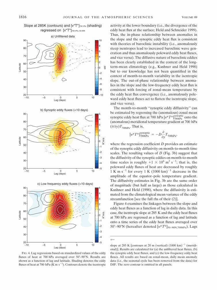
Figure 4 examines the linkages between the slope and

eddy heat fluxes as a function of lag in daily data. In this

case, the isentropic slope at 285 K and the eddy heat fluxes

at 700 hPa are regressed as a function of lag and latitude

onto a time series of the eddy heat fluxes averaged over

508–908N (hereafter denoted [y*T*]50–90N,700hPa). Lags

FIG. 4. Lag regressions based on standardized values of the eddy

fluxes of heat at 700 hPa averaged over 508–908N. Results are

shown as a function of lag and latitude. Shading denotes the eddy

fluxes of heat at 700 hPa (K m s21). Contours denote the isentropic

slope at 285 K [contours at 20 m (vertical) (1000 km)21 (meridi-

onal)]. Results are calculated for (a) the unfiltered heat fluxes, (b)

the synoptic eddy heat fluxes, and (c) the low-frequency eddy heat

fluxes. All results are based on zonal-mean, daily mean anomaly

data (i.e., the seasonal cycle has been removed from the data) for

DJF. The zero contour is omitted in all panels.


less than zero denote results that precede peak ampli-

tude in [y*T*]50–90N,700hPa, and vice versa. Figure 4a

shows results for unfiltered eddies, Fig. 4b for synoptic

eddies, and Fig. 4c for low-frequency eddies. Note that

the shading range in Fig. 4a is different from that used

in Figs. 4b,c.

By construction, in all panels the anomalous heat

fluxes (shading) peak at lag 0 and at middle to high

latitudes. The synoptic eddy heat fluxes are generally

positive at all lags (Fig. 4b); the low-frequency eddy heat

fluxes exhibit more pronounced quasi-periodic behavior

with a time scale of about 2 weeks (Fig. 4c; note the

negative regression coefficients at lags of about 27

and 17 days). The amplitudes of the low-frequency

eddy heat fluxes are roughly twice those of the synoptic

eddy heat fluxes.

The unfiltered heat fluxes are associated with opposite-

signed isentropic slope anomalies during the periods

before and after peak amplitude in mid- to high-latitude

wave generation (Fig. 4a). The approximately 5–10-day

period before peak wave generation is marked by in-

creases in the isentropic slope poleward of 508N; the

period following peak wave generation is marked by

decreases in the isentropic slope over middle and high

latitudes. Hence, as summarized schematically in Fig-

ures 1a and 1b, periods of anomalous tropospheric wave

generation are 1) preceded by anomalously steep isen-

tropic slopes consistent with anomalous instability of the

mean flow and 2) followed by anomalously flat isentro-

pic surfaces consistent with the stabilizing effect of the

resulting residual circulation (Fig. 1b). Note that the net

change in the isentropic slope is very small when inte-

grated over lags 210 to 110, as expected from the weak

monthly mean regression coefficients given by the solid

line in Fig. 3a.

The synoptic eddy heat fluxes are dominated by pos-

itive correlations with the isentropic slope that peak

several days before lag 0 (Fig. 4b). Lag correlations do

not prove causality. Nevertheless, the peak in the lag

correlations before lag 0 is consistent with forcing of the

synoptic eddy heat fluxes by variability in the isentropic

slope (i.e., anomalously steep slopes lead to anomalous

wave generation). In contrast, the rapid damping of the

slope anomalies after lag 0 is consistent with forcing of

the slope by the anomalous wave breaking aloft (see also

Fig. 1b).

The low-frequency eddy heat fluxes are dominated by

large negative correlations with the isentropic slope at

positive lag (Fig. 4c). Again, the negative tendency in

the slope after lag 0 is consistent with forcing of the slope

by the anomalous wave breaking aloft. The compara-

tively weak positive correlations at negative lag are lim-

ited to very high latitudes. The apparent precursor in

the slope in Fig. 4c may reflect the sensitivity of low-

frequency eddies to the configuration of the flow, but it

is also due at least in part to the periodicity inherent in

the low-frequency eddy forcing (i.e., the positive slope

anomalies between days 25 and 0 follow a period of neg-

ative heat fluxes anomalies between days 25 and 210).

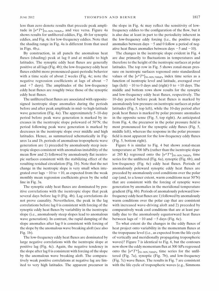
The changes in the isentropic slope evident in Fig. 4

are due primarily to fluctuations in temperatures and

therefore to the height of the isentropic surfaces at polar

latitudes. The top row in Fig. 5 shows zonal-mean pres-

sure on isentropic surfaces regressed onto standardized

values of the [y*T*]50–90N,700hPa index time series as a

function of isentropic level and latitude, averaged over

lags (left) 210 to 0 days and (right) 0 to 110 days. The

middle and bottom rows show results for the synoptic

and low-frequency eddy heat fluxes, respectively. The

10-day period before peak heat fluxes is marked by

anomalously low pressure on isentropic surfaces at polar

latitudes (Fig. 5, top left), while the 10-day period after

peak heat fluxes is marked by polar pressure anomalies

in the opposite sense (Fig. 5, top right). As anticipated

from Fig. 4, the precursor in the polar pressure field is

most pronounced for the synoptic eddy fluxes (Fig. 5,

middle left), whereas the response in the polar pressure

field is most apparent for the low-frequency eddy fluxes

(Fig. 5, bottom right).

Figure 6 is similar to Fig. 4 but shows zonal-mean

temperature at 700 hPa (rather than the isentropic slope

at 285 K) regressed onto the [y*T*]50–90N,700hPa time

series for the unfiltered (Fig. 6a), synoptic (Fig. 6b), and

low-frequency (Fig. 6c) eddy heat fluxes. Periods of

anomalously poleward synoptic eddy heat fluxes are

preceded by anomalously cool conditions over the polar

cap (and, to a lesser extent, warm conditions near 508N)

that are consistent with the forcing of synoptic wave

generation by anomalies in the meridional temperature

gradient (Fig. 6b). Periods of anomalously poleward low-

frequency eddy heat fluxes are 1) followed by anomalously

warm conditions over the polar cap that are consistent

with increased wave-driving aloft and 2) preceded by

comparatively weak cool conditions that are at least par-

tially due to the anomalously equatorward heat fluxes

between lags of 210 and 25 days (Fig. 6c).

To what extent do the changes in the eddy fluxes of

heat project onto variability in the momentum fluxes at

the tropopause level (i.e., as expected from the life cycle

of vertically and meridionally propagating tropospheric

waves)? Figure 7 is identical to Fig. 6, but the contours

now show the eddy momentum flux at 300 hPa regressed

onto the [y*T*]50–90N,700hPa time series for the unfil-

tered (Fig. 7a), synoptic (Fig. 7b), and low-frequency

(Fig. 7c) wave fluxes. The results in Fig. 7 are consistent

with the life cycle of tropospheric waves (e.g., Simmons


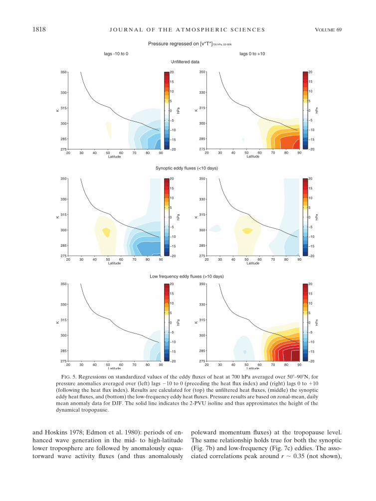
and Hoskins 1978; Edmon et al. 1980): periods of en-

hanced wave generation in the mid- to high-latitude

lower troposphere are followed by anomalously equa-

torward wave activity fluxes (and thus anomalously

poleward momentum fluxes) at the tropopause level.

The same relationship holds true for both the synoptic

(Fig. 7b) and low-frequency (Fig. 7c) eddies. The asso-

ciated correlations peak around r ; 0.35 (not shown),

FIG. 5. Regressions on standardized values of the eddy fluxes of heat at 700 hPa averaged over 508–908N, for

pressure anomalies averaged over (left) lags 210 to 0 (preceding the heat flux index) and (right) lags 0 to 110

(following the heat flux index). Results are calculated for (top) the unfiltered heat fluxes, (middle) the synoptic

eddy heat fluxes, and (bottom) the low-frequency eddy heat fluxes. Pressure results are based on zonal-mean, daily

mean anomaly data for DJF. The solid line indicates the 2-PVU isoline and thus approximates the height of the

dynamical tropopause.


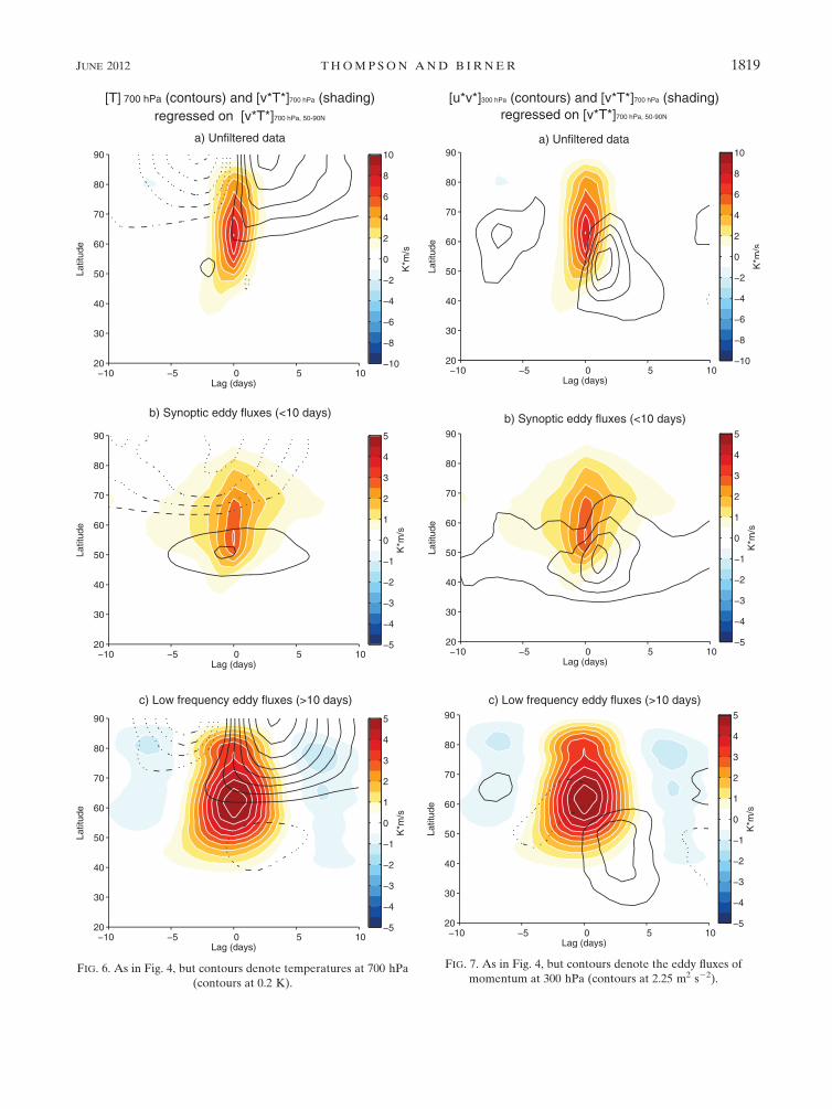
FIG. 6. As in Fig. 4, but contours denote temperatures at 700 hPa

(contours at 0.2 K).

FIG. 7. As in Fig. 4, but contours denote the eddy fluxes of

momentum at 300 hPa (contours at 2.25 m2 s22).


and thus variations in the generation of wave activity

over mid to high latitudes account for at most approxi-

mately 10% of the day-to-day variance in the momen-

tum fluxes at middle latitudes. The remaining fraction is

likely due to either 1) internal variability in the mo-

mentum fluxes that is independent of variability in the

heat fluxes and/or 2) anomalous wave generation that is

not captured by the heat flux index used to generate the

figure.

The most important result in this section is the ap-

parent causal linkage between variability in the isen-

tropic slope and the generation of baroclinic waves.

Such a linkage is widely accepted in the context of the

climatological-mean circulation (i.e., baroclinic waves de-

velop primarily in regions of large baroclinicity). But

to our knowledge, such a linkage has not been clearly

demonstrated in the context of day-to-day and month-

to-month variability in the isentropic slope. Both the

sign and lead/lag nature of the results suggest a causal

relationship between the slope and the synoptic eddy

heat fluxes: the synoptic eddy fluxes of heat are anom-

alously downgradient and thus cannot drive the at-

tendant changes in the temperature field (Figs. 3a, 4b,

and 6b); the largest synoptic eddy flux anomalies lag

variability in the isentropic slope by several days (Fig.

4b). The linkages are highly significant (Fig. 3a) and the

precursor in the temperature field (Fig. 6a) cannot be

explained as an artifact of the (quasi-random) period-

icity inherent in the eddy forcing. In the following sec-

tion we will discuss the implications of the central results

for large-scale climate variability.

4. Discussion

The influence of the mean flow on the eddy fluxes of

heat and momentum can be viewed via two processes:

1) via wave propagation and dissipation in the free tro-

posphere and 2) via the generation of wave activity near

the earth’s surface. Both are clearly important in the

earth’s atmosphere. The configuration of the mean flow

determines the ‘‘index of refraction’’ for wave propa-

gation and the regions for wave breaking. The tropo-

spheric isentropic slope affects the generation of wave

activity in the lower troposphere as well as the charac-

teristics of wave propagation. Here we have focused

on the relationship between the slope of the isentropic

surfaces and the generation of wave activity in the lower

troposphere.

The isentropic slope is related to the potential energy

available to generate atmospheric eddies (e.g., Lorenz

1955; O’Gorman 2010), is of fundamental importance

for baroclinic wave generation (e.g., Stone 1978; Stone

and Nemet 1996), is intimately related to the growth rate

in theories of baroclinic instability (e.g., Lindzen and

Farrell 1980), and is directly related to the meridional

PV gradient and thus the index of refraction for wave

propagation (section 3). The results in section 3 reveal

three aspects of the linkages between the isentropic slope

and the wave fluxes of heat and momentum: 1) periods of

increased isentropic slope are linked to enhanced gen-

eration of synoptic eddies near the surface; 2) enhanced

generation of wave activity near the surface is linked to

a rapid flattening of the isentropic slope that is consistent

with increased wave dissipation aloft; and 3) enhanced

generation of wave activity near the surface is followed by

several days by anomalous eddy momentum fluxes aloft

that are consistent with the life cycle of vertically and

horizontally propagating waves. The results suggest that

about 10% of the variance in the upper-tropospheric

wave fluxes of momentum is linked directly to variability

in the source of wave activity in the mid- to high-latitude

lower troposphere.

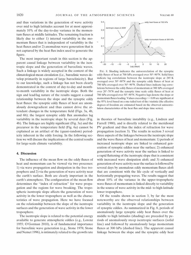
Of the results shown in section 3, by far the most

noteworthy are the observed relationships between

variability in the isentropic slope and the generation

of synoptic eddies. As summarized in Fig. 8, periods of

anomalously large synoptic eddy heat fluxes over the

middle to high latitudes (shading) are preceded by pe-

riods of anomalously steep isentropic surfaces (solid

line) and followed by anomalously large momentum

fluxes at 300 hPa (dashed line). The apparent causal

linkage between the slope and the synoptic eddy heat

FIG. 8. Shading indicates the autocorrelation of the synoptic

eddy fluxes of heat at 700 hPa averaged over 508–908N. Solid lines

indicate lag correlations between the isentropic slope at 285 K

averaged over 508–908N and the synoptic eddy fluxes of heat at

700 hPa averaged over 508–908N. Dashed lines indicate lag corre-

lations between the eddy fluxes of momentum at 300 hPa averaged

over 208–708N and the synoptic time scale eddy fluxes of heat at

700 hPa averaged over 508–908N. Negative lags denote the slope or

momentum fluxes leading. Values exceeding r 5 0.09 are significant at

the 95% level based on a one-tailed test of the t statistic (the effective

degrees of freedom are estimated based on the observed autocorre-

lation characteristics of the heat flux and slope time series).


fluxes is consistent with the dynamics of developing

baroclinic waves (Stone 1978; Stone and Nemet 1996),

the close relationship between available potential en-

ergy and the amplitude of the wave component of the

flow (e.g., O’Gorman 2010), and the ‘‘macroturbulent’’

view of atmospheric eddies (e.g., Held 1999). As noted

above such a linkage has been demonstrated in the

context of the long-term mean circulation (e.g., Kushner

and Held 1998) and is presumed to underlie the dy-

namics of the annular modes (e.g., Robinson 1991, 2000),

but has not been demonstrated conclusively in the con-

text of day-to-day and month-to-month variability in the

isentropic slope. We were unable to find similarly robust

evidence of a direct causal linkage between variations in

the mean flow and the eddy fluxes of momentum.

The observed relationships between variations in the

isentropic slope and the generation of synoptic eddies

have potentially important implications for understand-

ing the extratropical circulation response to a range of

forcings. The following are some examples:

1) The annular modes are theorized to derive in part

from feedbacks between the momentum fluxes aloft,

lower-tropospheric baroclinicity, and the generation

of baroclinic waves (e.g., Robinson 2000; Lorenz and

Hartmann 2001, 2003). The annular mode dynamics

envisioned in Robinson (1991) and the correspond-

ing feedback loop articulated in Robinson (2000)

hinge on the forcing of anomalous wave activity by

changes in the lower-tropospheric isentropic slope.

The results in section 3 provide observational sup-

port for such forcing.

2) A range of forcings are predicted to drive changes in

the storm tracks via their influence on the barocli-

nicity and thus isentropic slope in the extratropics.

Increasing greenhouse gases are predicted to steepen

the extratropical isentropic slope via changes in both

the horizontal temperature gradient and static sta-

bility (e.g., Kushner et al. 2001; Yin 2005; Frierson

2006; Lu et al. 2008, 2010; Chen et al. 2010; O’Gorman

2010; Scaife et al. 2012; Butler et al. 2011); Antarctic

ozone depletion is predicted to steepen the isentropic

slope at southern high latitudes through the radiative

effects of the Antarctic ozone hole (Grise et al. 2009);

and midlatitude sea surface temperatures anomalies

are predicted to perturb surface baroclinicity in the

vicinity of the extratropical storm tracks (e.g., Kushnir

et al. 2002, and references therein; Brayshaw et al.

2008). The results in section 3 provide observational

support for a robust response in tropospheric wave

generation to such changes in the isentropic slope.

3) Finally, wave-driven changes in the stratospheric

circulation (e.g., sudden stratospheric warmings) are

expected to drive variability in the tropospheric isen-

tropic slope due to the downward penetrating mass

circulation (e.g., Haynes et al. 1991; Song and

Robinson 2004; Thompson et al. 2006). The relation-

ships between stratospheric variability and the tro-

pospheric isentropic slope are considered in Fig. 9.

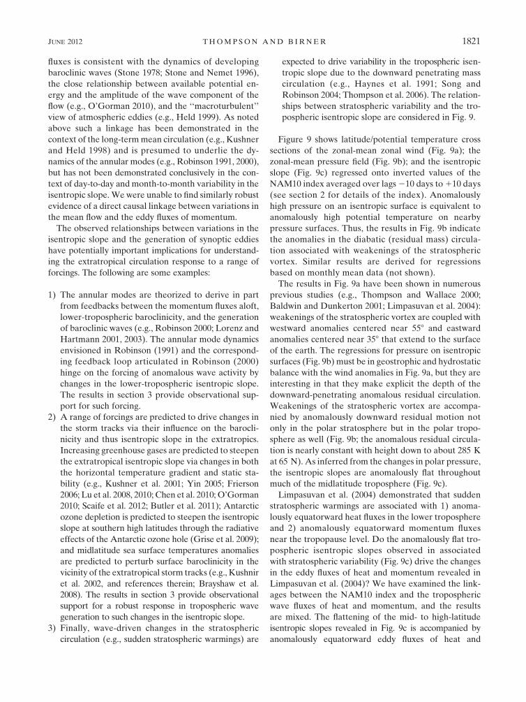
Figure 9 shows latitude/potential temperature cross

sections of the zonal-mean zonal wind (Fig. 9a); the

zonal-mean pressure field (Fig. 9b); and the isentropic

slope (Fig. 9c) regressed onto inverted values of the

NAM10 index averaged over lags 210 days to 110 days

(see section 2 for details of the index). Anomalously

high pressure on an isentropic surface is equivalent to

anomalously high potential temperature on nearby

pressure surfaces. Thus, the results in Fig. 9b indicate

the anomalies in the diabatic (residual mass) circula-

tion associated with weakenings of the stratospheric

vortex. Similar results are derived for regressions

based on monthly mean data (not shown).

The results in Fig. 9a have been shown in numerous

previous studies (e.g., Thompson and Wallace 2000;

Baldwin and Dunkerton 2001; Limpasuvan et al. 2004):

weakenings of the stratospheric vortex are coupled with

westward anomalies centered near 558 and eastward

anomalies centered near 358 that extend to the surface

of the earth. The regressions for pressure on isentropic

surfaces (Fig. 9b) must be in geostrophic and hydrostatic

balance with the wind anomalies in Fig. 9a, but they are

interesting in that they make explicit the depth of the

downward-penetrating anomalous residual circulation.

Weakenings of the stratospheric vortex are accompa-

nied by anomalously downward residual motion not

only in the polar stratosphere but in the polar tropo-

sphere as well (Fig. 9b; the anomalous residual circula-

tion is nearly constant with height down to about 285 K

at 65 N). As inferred from the changes in polar pressure,

the isentropic slopes are anomalously flat throughout

much of the midlatitude troposphere (Fig. 9c).

Limpasuvan et al. (2004) demonstrated that sudden

stratospheric warmings are associated with 1) anoma-

lously equatorward heat fluxes in the lower troposphere

and 2) anomalously equatorward momentum fluxes

near the tropopause level. Do the anomalously flat tro-

pospheric isentropic slopes observed in associated

with stratospheric variability (Fig. 9c) drive the changes

in the eddy fluxes of heat and momentum revealed in

Limpasuvan et al. (2004)? We have examined the link-

ages between the NAM10 index and the tropospheric

wave fluxes of heat and momentum, and the results

are mixed. The flattening of the mid- to high-latitude

isentropic slopes revealed in Fig. 9c is accompanied by

anomalously equatorward eddy fluxes of heat and


momentum at mid- to high latitudes (not shown). But the

largest tropospheric eddy heat flux anomalies are due

primarily to low-frequency eddies (rather than synoptic

eddies, as inferred from Figs. 3 and 4). And the largest

tropospheric eddy momentum flux anomalies precede

the largest changes in the eddy heat fluxes (rather than

follow, as inferred from Fig. 7). The linkages between

stratospheric variability and the tropospheric mass cir-

culation, isentropic slope, and wave fluxes of heat and

momentum will be examined in detail in a future study.

Acknowledgments. We thank Walter Robinson and

an anonymous reviewer for their insightful and helpful

reviews. David W. J. Thompson and Thomas Birner are

supported by the NSF Climate Dynamics Program.

REFERENCES

Baldwin, M. P., and T. J. Dunkerton, 2001: Stratospheric harbin-

gers of anomalous weather regimes. Science, 294, 581–584.

——, and D. W. J. Thompson, 2009: A critical comparison of

stratosphere–troposphere coupling indices. Quart. J. Roy.

Meteor. Soc., 135, 1661–1672.

Brayshaw, D. J., B. Hoskins, and M. Blackburn, 2008: The storm-

track response to idealized SST perturbations in an aqua-

planet GCM. J. Atmos. Sci., 65, 2842–2860.

Butler, A. H., D. W. J. Thompson, and T. Birner, 2011: Isentropic

slopes, down-gradient eddy fluxes, and the extratropical at-

mospheric circulation response to tropical tropospheric heat-

ing. J. Atmos. Sci., 68, 2292–2305.

Chen, G., R. A. Plumb, and J. Lu, 2010: Sensitivities of zonal mean

atmospheric circulation to SST warming in an aqua-planet model.

Geophys. Res. Lett., 37, L12701, doi:10.1029/2010GL043473.

Dee, D. P., and Coauthors, 2011: The ERA-Interim reanalysis:

Configuration and performance of the data assimilation system.

Quart. J. Roy. Meteor. Soc., 137, 553–597, doi:10.1002/qj.828.

Edmon, H. J., Jr., B. J. Hoskins, and M. E. Mclntyre, 1980: Eliassen–

Palm cross sections for the troposphere. J. Atmos. Sci., 37, 2600–

2615.

Frierson, D. M. W., 2006: Robust increases in midlatitude static

stability in simulations of global warming. Geophys. Res. Lett.,

33, L24816, doi:10.1029/2006GL027504.

Grise, K. M., D. W. J. Thompson, and P. M. Forster, 2009: On the

role of radiative processes in stratosphere–troposphere cou-

pling. J. Climate, 22, 4154–4161.

Haynes, P. H., M. E. Mclntyre, T. G. Shepherd, C. J. Marks, and

K. P. Shine, 1991: On the ‘‘downward control’’ of extratropical

diabatic circulations by eddy-induced mean zonal forces.

J. Atmos. Sci., 48, 651–680.

Held, I. M., 1999: The macroturbulence of the troposphere. Tellus,

51, 59–70.

——, and T. Schneider, 1999: The surface branch of the zonally

averaged mass transport circulation in the troposphere.

J. Atmos. Sci., 56, 1688–1697.

Holton, J. R., 2004: An Introduction to Dynamic Meteorology. 4th

ed. Academic Press, 535 pp.

Kushner, P. J., and I. M. Held, 1998: A direct test, using atmo-

spheric data, of a method for estimating oceanic diffusivity.

Geophys. Res. Lett., 25, 4213–4216.

FIG. 9. Regressions based on inverted and standardized values of

the NAM index at 10 hPa: (top) the zonal-mean zonal wind,

(middle) the pressure on isentropic surfaces, and (bottom) the is-

entropic slope. Results are based on zonal-mean, daily mean

anomaly data for DJF. Results are averaged over lags 210 days

(preceding the NAM10 index) to 110 days (following the

NAM10 index). The solid line indicates the 2-PVU isoline and

thus approximates the height of the dynamical tropopause.


——, ——, and T. L. Delworth, 2001: Southern Hemisphere at-

mospheric circulation response to global warming. J. Climate,

14, 2238–2249.

Kushnir, Y., W. A. Robinson, I. Blade, N. M. J. Hall, S. Peng, and

R. Sutton, 2002: Atmospheric GCM response to extratropical

SST anomalies: synthesis and evaluation. J. Climate, 15, 2233–

2256.

Lau, N.-C., H. Tennekes, and J. M. Wallace, 1978: Maintenance of

the momentum flux by transient eddies in the upper tropo-

sphere. J. Atmos. Sci., 35, 139–147.

Lim, G. H., and J. M. Wallace, 1991: Structure and evolution of

baroclinic waves as inferred from regression analysis. J. At-

mos. Sci., 48, 1718–1732.

Limpasuvan, V., D. W. J. Thompson, and D. L. Hartmann, 2004:

The life cycle of the Northern Hemisphere sudden strato-

spheric warmings. J. Climate, 17, 2584–2596.

Lindzen, R. S., and B. F. Farrell, 1980: A simple approximate re-

sult for the maximum growth rate of baroclinic instabilities.

J. Atmos. Sci., 37, 1648–1654.

Lorenz, D. J., and D. L. Hartmann, 2001: Eddy–zonal flow feed-

back in the Southern Hemisphere. J. Atmos. Sci., 58, 3312–

3327.

——, and ——, 2003: Eddy–zonal flow feedback in the Northern

Hemisphere winter. J. Climate, 16, 1212–1227.

Lorenz, E. N., 1955: Available potential energy and the mainte-

nance of the general circulation. Tellus, 7, 157–167.

Lu, J., G. Chen, and D. M. W. Frierson, 2008: Response of the zonal

mean atmospheric circulation to El Nino versus global warming.

J. Climate, 21, 5835–5851.

——, ——, and ——, 2010: The position of the midlatitude storm

track and eddy-driven westerlies in aquaplanet AGCMs.

J. Atmos. Sci., 67, 3984–4000.

O’Gorman, P. A., 2010: Understanding the varied response of the

extratropical storm tracks to climate change. Proc. Natl. Acad.

Sci. USA, 107, 19 176–19 180.

Robinson, W. A., 1991: The dynamics of the zonal index in a simple

model of the atmosphere. Tellus, 43A, 295–305.

——, 2000: A baroclinic mechanism for the eddy feedback on the

zonal index. J. Atmos. Sci., 57, 415–422.

——, 2006: On the self-maintenance of midlatitude jets. J. Atmos.

Sci., 63, 2109–2122.

Scaife, A. A., and Coauthors, 2012: Climate change projections and

stratosphere–troposphere coupling. Climate Dyn., 38, 2089–

2097, doi:10.1007/s00382-011-1080-7.

Simmons, A. J., and B. J. Hoskins, 1978: The life cycles of some

nonlinear baroclinic waves. J. Atmos. Sci., 35, 414–432.

Song, Y., and W. A. Robinson, 2004: Dynamical mechanisms for

stratospheric influences on the troposphere. J. Atmos. Sci., 61,

1711–1725.

Stone, P. H., 1978: Baroclinic adjustment. J. Atmos. Sci., 35, 561–571.

——, and B. Nemet, 1996: Baroclinic adjustment: A comparison

between theory, observations, and models. J. Atmos. Sci., 53,

1663–1674.

Thompson, D. W. J., and J. M. Wallace, 2000: Annular modes in the

extratropical circulation. Part I: Month-to-month variability.

J. Climate, 13, 1000–1016.

——, J. C. Furtado, and T. G. Shepherd, 2006: On the tropospheric

response to anomalous stratospheric wave drag and radiative

heating. J. Atmos. Sci., 63, 2616–2629.

Vallis, G. K., 2006. Atmospheric and Oceanic Fluid Dynamics.

Cambridge University Press, 745 pp.

Yin, J. H., 2005: A consistent poleward shift of the storm tracks in

simulations of 21st century climate. Geophys. Res. Lett., 32,

L18701, doi:10.1029/2005GL023684.


Documents

On the Linkages between the Tropospheric Isentropic Slope