Embed Size (px)
Citation preview
JOTA manuscript No.(will be inserted by the editor)
On the local convergence analysis
of the Gradient Sampling method
Elias Salomao Helou · Sandra A. Santos ·
Lucas E. A. Simoes
Received: date / Accepted: date
Elias Salomao Helou was partially supported by FAPESP grant 2013/07375-0 and by CNPq
grant 311476/2014-7.
Sandra A. Santos was partially supported by CNPq grant 304032/2010-7, FAPESP grants
2013/05475-7 and 2013/07375-0 and PRONEX Optimization.
Lucas E. A. Simoes was supported by FAPESP grant 2013/14615-7.
Elias Salomao Helou
Institute of Mathematical Sciences and Computation, University of Sao Paulo.
Sao Carlos - SP, Brazil.
E-mail: [email protected]
Sandra A. Santos
Department of Applied Mathematics, University of Campinas.
Campinas - SP, Brazil.
E-mail: [email protected]
Lucas E. A. Simoes
Department of Applied Mathematics, University of Campinas.
Campinas - SP, Brazil.
E-mail: [email protected]

2 Elias Salomao Helou et al.
Abstract The Gradient Sampling method is a recently developed tool for
solving unconstrained nonsmooth optimization problems. Using just first order
information about the objective function, it generalizes the steepest descent
method, one of the most classical methods to minimize a smooth function. This
manuscript aims at determining under which circumstances one can expect the
same local convergence result of the Cauchy method for the Gradient Sampling
algorithm. Additionally, at the end of this study, we show how to practically
accomplish the required hypotheses during the execution of the algorithm.
Keywords nonsmooth nonconvex optimization · gradient sampling · local
convergence · unconstrained minimization
Mathematics Subject Classification (2000) 90C30 · 65K05
1 Introduction
In the past fifteen years an algorithm known as Gradient Sampling (GS) has
gained attention because of its good numerical results in solving nonsmooth
optimization problems (specially for nonconvex objective functions) [1,2]. A
strong appeal of the referred method is its intuitive functioning, which uses
just first order information to find a descent direction and performs a line
search procedure to find out the next iterate. Different from other optimization
algorithms, it has a nondeterministic approach, since it randomly samples
points around the current iterate in order to obtain a rich set of gradients to
compute the search direction. Consequently, a good movement towards the
solution is directly linked to a good set of sampled points.
On the local convergence analysis of the Gradient Sampling method 3
In 2007, Kiwiel introduced a nonnormalized version of GS [3], which can
be viewed as a generalization of the well known steepest descent method for
smooth functions. Hence, it suggests that, in the best case scenario, the Gra-
dient Sampling will have the same local convergence of the Cauchy method.
Although this is reasonable to expect, for the best of our knowledge, there is
no proof in the literature of local convergence rates for the GS method nor a
clarification of hypotheses under which this can be established.
This theoretical paper has the goal to prove that, under special circum-
stances, one can achieve linear convergence of the GS method towards the
optimal function value of the optimization problem. Moreover, we justify the
hypotheses made along the manuscript with illustrative examples, which help
us to understand when such a behavior cannot be expected.
The outline of this study is as follows. Section 2 presents the theoretical
background and the GS algorithm. Section 3 shows an example that helps us to
understand what kind of hypotheses are needed to obtain a good performance
from the method. Section 4 is devoted to the theoretical results that prove
linear convergence of the algorithm. Section 5 exhibits a practical implication
of our study to the GS method with illustrative examples and comparative
results. The final section is dedicated to the conclusions.
For clarity, we present some notations that appear along this manuscript:
– coX is the convex hull of X ;
– X# is the cardinality of X ;

4 Elias Salomao Helou et al.
– B(x, r) and B(x, r) are, respectively, the Euclidean open and closed balls
with center at x and radius r;
– ‖ · ‖ is the Euclidean norm in Rn;
– e is a vector of appropriate dimension with ones in all entries;
– PV(x) is the orthogonal projection of x into the vector space V.
2 GS algorithm
The GS method has the aim to solve the following unconstrained optimization
problem
minx∈Rn
f(x), (1)
where f : Rn → R is a nonsmooth locally Lipschitz function, continuously
differentiable in an open dense subset D ⊂ Rn. The function f can be either
convex or nonconvex.
For objective functions that satisfy the properties required above, it is
possible to define a generalization of the so called derivatives for smooth func-
tions [4].
Definition 2.1 (Subdifferential set, subgradient, stationary point) The
set given by
∂f(x) := co
{limj→∞
∇f(xj) | xj → x, xj ∈ D}
is called the Clarke’s subdifferential set for f at x and any v ∈ ∂f(x) is known
as a subgradient of f at x. Moreover, if 0 ∈ ∂f(x), then we say that x is a
stationary point for f .
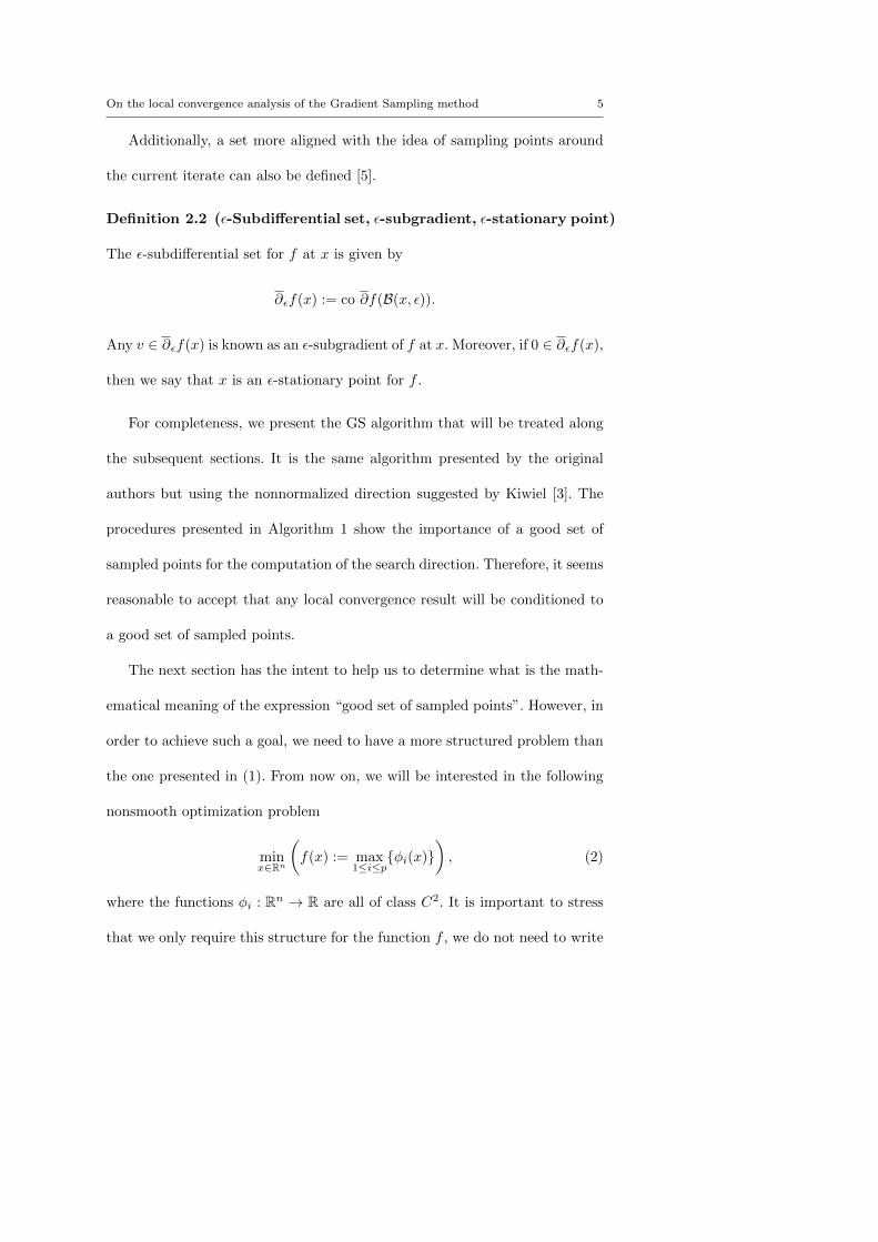
On the local convergence analysis of the Gradient Sampling method 5
Additionally, a set more aligned with the idea of sampling points around
the current iterate can also be defined [5].
Definition 2.2 (ε-Subdifferential set, ε-subgradient, ε-stationary point)
The ε-subdifferential set for f at x is given by
∂εf(x) := co ∂f(B(x, ε)).
Any v ∈ ∂εf(x) is known as an ε-subgradient of f at x. Moreover, if 0 ∈ ∂εf(x),
then we say that x is an ε-stationary point for f .
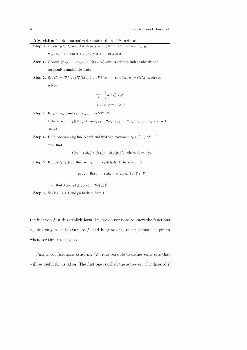
For completeness, we present the GS algorithm that will be treated along
the subsequent sections. It is the same algorithm presented by the original
authors but using the nonnormalized direction suggested by Kiwiel [3]. The
procedures presented in Algorithm 1 show the importance of a good set of
sampled points for the computation of the search direction. Therefore, it seems
reasonable to accept that any local convergence result will be conditioned to
a good set of sampled points.
The next section has the intent to help us to determine what is the math-
ematical meaning of the expression “good set of sampled points”. However, in
order to achieve such a goal, we need to have a more structured problem than
the one presented in (1). From now on, we will be interested in the following
nonsmooth optimization problem
minx∈Rn
(f(x) := max
1≤i≤p{φi(x)}
), (2)
where the functions φi : Rn → R are all of class C2. It is important to stress
that we only require this structure for the function f , we do not need to write
6 Elias Salomao Helou et al.
Algorithm 1: Nonnormalized version of the GS method.Step 0. Given x0 ∈ D, m ∈ N with m ≥ n+ 1, fixed real numbers ν0, ε0,
νopt, εopt > 0 and 0 < θν , θε, γ, β < 1, set k = 0.
Step 1. Choose{xk,1, . . . , xk,m
}⊂ B(xk, εk) with randomly, independently and
uniformly sampled elements.
Step 2. Set Gk = [∇f(xk) ∇f(xk,1) . . .∇f(xk,m)] and find gk = Gkλk, where λk
solves
minλ
1
2λTGTkGkλ
s.t. eTλ = 1, λ ≥ 0.
Step 3. If νk < νopt and εk < εopt, then STOP!
Otherwise, if ‖gk‖ < νk, then εk+1 = θεεk, νk+1 = θννk, xk+1 = xk and go to
Step 6.
Step 4. Do a backtracking line search and find the maximum tk ∈ {1, γ, γ2, . . .}
such that
f(xk + tkdk) < f(xk)− βtk‖gk‖2, where dk = −gk.
Step 5. If xk + tkdk ∈ D, then set xk+1 = xk + tkdk. Otherwise, find
xk+1 ∈ B(xk + tkdk,min{tk, εk}‖dk‖) ∩ D,
such that f(xk+1) ≤ f(xk)− βtk‖gk‖2.
Step 6. Set k ← k + 1 and go back to Step 1.
the function f in this explicit form, i.e., we do not need to know the functions
φi, but only need to evaluate f , and its gradient, at the demanded points
whenever the latter exists.
Finally, for functions satisfying (2), it is possible to define some sets that
will be useful for us latter. The first one is called the active set of indices of f
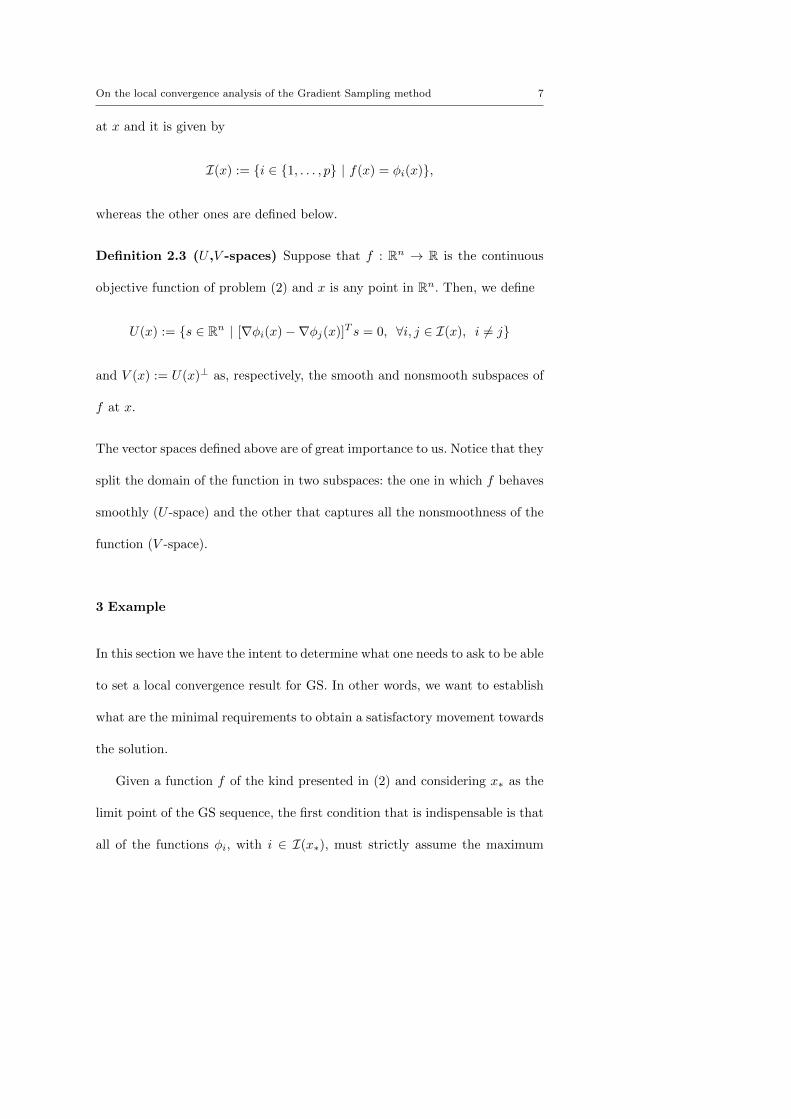
On the local convergence analysis of the Gradient Sampling method 7
at x and it is given by
I(x) := {i ∈ {1, . . . , p} | f(x) = φi(x)},
whereas the other ones are defined below.
Definition 2.3 (U ,V -spaces) Suppose that f : Rn → R is the continuous
objective function of problem (2) and x is any point in Rn. Then, we define
U(x) := {s ∈ Rn | [∇φi(x)−∇φj(x)]T s = 0, ∀i, j ∈ I(x), i 6= j}
and V (x) := U(x)⊥ as, respectively, the smooth and nonsmooth subspaces of
f at x.
The vector spaces defined above are of great importance to us. Notice that they
split the domain of the function in two subspaces: the one in which f behaves
smoothly (U -space) and the other that captures all the nonsmoothness of the
function (V -space).
3 Example
In this section we have the intent to determine what one needs to ask to be able
to set a local convergence result for GS. In other words, we want to establish
what are the minimal requirements to obtain a satisfactory movement towards
the solution.
Given a function f of the kind presented in (2) and considering x∗ as the
limit point of the GS sequence, the first condition that is indispensable is that
all of the functions φi, with i ∈ I(x∗), must strictly assume the maximum

8 Elias Salomao Helou et al.
at least at one of the sampled points or at the current iterate. In a more
rigorous way, we are saying that, for a good movement towards the solution
at some fixed iteration k, given any i ∈ I(x∗), there must be xk,j , for some
j ∈ {0, . . . ,m} (here, and from now on, we define xk,0 := xk), such that
φi(xk,j) > φs(xk,j), for any s ∈ {1, . . . , p} \ {i}. (Hφ)
To highlight the plausibility of this hypothesis, we present an example where
the absence of this assumption causes a bad GS behavior.
Let us consider a two-dimensional function f : R2 → R, with
f(x) = max {φ1(x), φ2(x), φ3(x)} ,
where, for x = [ξ1 ξ2]T , we have
φ1(x) = ξ1 + ξ2, φ2(x) = −2ξ1 + ξ2 and φ3(x) = ξ1 − 2ξ2.
Clearly, it is a convex function with x∗ = 0 as its global minimizer. Further-
more, the lowest function value is given by f(x∗) = 0.
Suppose we want to start an iteration of the GS method with
x0 =[0.5l 0.52l
]T, for any fixed l ∈ N.
Moreover, we assume that the method has sampled in such a way that
f(x0,i) = φ2(x0,i), ∀i ∈ {1, 2, 3} (assuming m = 3).
Consequently, the function φ3 does not assume the maximum at the sampled
points nor at x0. Step 2 returns us g0 = [0 1]T . Assuming that ν0 = ε0 = 10−1
On the local convergence analysis of the Gradient Sampling method 9
and εopt = νopt = 10−6, the method does not stop neither jumps from Step 3
to Step 6.
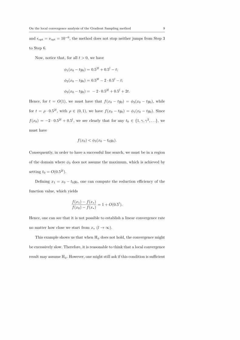
Now, notice that, for all t > 0, we have
φ1(x0 − tg0) = 0.52l + 0.5l − t;
φ2(x0 − tg0) = 0.52l − 2 · 0.5l − t;
φ3(x0 − tg0) = − 2 · 0.52l + 0.5l + 2t.
Hence, for t = O(1), we must have that f(x0 − tg0) = φ3(x0 − tg0), while
for t = ρ · 0.52l, with ρ ∈ (0, 1), we have f(x0 − tg0) = φ1(x0 − tg0). Since
f(x0) = −2 · 0.52l + 0.5l, we see clearly that for any t0 ∈ {1, γ, γ2, . . .}, we
must have
f(x0) < φ3(x0 − t0g0).
Consequently, in order to have a successful line search, we must be in a region
of the domain where φ3 does not assume the maximum, which is achieved by
setting t0 = O(0.52l).
Defining x1 = x0 − t0g0, one can compute the reduction efficiency of the
function value, which yields
f(x1)− f(x∗)
f(x0)− f(x∗)= 1 +O(0.5l).
Hence, one can see that it is not possible to establish a linear convergence rate
no matter how close we start from x∗ (l→∞).
This example shows us that when Hφ does not hold, the convergence might
be excessively slow. Therefore, it is reasonable to think that a local convergence
result may assume Hφ. However, one might still ask if this condition is sufficient
10 Elias Salomao Helou et al.
for our goal. Unfortunately, Hφ is not enough for reaching our purposes, as
the size of the sampling radius plays a key role as well (see Sections 4 and 5).
Indeed, an additional condition must be taken into account: a restriction over
the value of
τk := max1≤i≤m
{‖xk,i − xk‖}. (3)
We state that assuming Hφ and τk ≤ T‖xk − x∗‖2, for some small enough
T > 0, is sufficient to obtain a linear convergence rate of the function values.
Before we proceed with the expected proofs, we need to make an observa-
tion. The local convergence theory developed here is only applicable to func-
tions that have local minimizers x∗ that satisfy dim{U(x∗)} 6= 0. We justify
this statement by looking back at the example just exhibited. We have seen
that the lack of fulfillment of Hφ leaves us with a bad behavior of the GS
method. However, if Hφ were valid for this specific example, it would yield
that g0 = 0. So, by Step 3, we would have x1 = x0. Hence, with or without
the condition Hφ, the theory we have developed here says nothing about the
local convergence whenever V (x∗) = Rn.
4 Convergence results
In this section we have established a local convergence result for the nonnor-
malized GS method under the more structured case defined in (2). In other
words, we find R ∈ (0, 1) such that, for some infinite index set K ⊂ N, we have
f(xk+1)− f(x∗) ≤ R [f(xk)− f(x∗)] , ∀k ∈ K.

On the local convergence analysis of the Gradient Sampling method 11
For that goal, we need to assume a condition upon the derivatives of the
functions φi [6].
Assumption 1 For all x ∈ Rn with |I(x)| ≥ 2, the gradients {∇φi(x)}i∈I(x)
compose an affinely independent set, that is,
∑i∈I(x)
αi∇φi(x) = 0 and∑i∈I(x)
αi = 0 ⇐⇒ αi = 0, ∀i ∈ I(x).
It is not hard to show that if Assumption 1 holds, then I(x)# ≤ n + 1.
Additionally, this information together with dim{U(x∗)} ≥ 1 give us that
I(x)# ≤ n.
Notice that, by the way the subdifferential set is defined, all functions with
the representation given by (2) have the following property
∂f(x) := co {∇φi(x) | i ∈ I(x)} .
Consequently, supposing that x∗ is a stationary point for f , Assumption 1 tells
us that there is only one convex combination of ∇φi(x∗), with i ∈ I(x∗), such
that it generates the null vector.
With the considerations made above, we are ready to present the results
that will culminate in the main theorem. For an easier exposition of the
statements, from now on we will assume that x∗ is always a local minimizer
for the function f (with dim{U(x∗)} ≥ 1). Moreover, we will consider that
I(x∗)# ≥ 2, since otherwise the convergence would be to a point where f is
smooth, which is not the case of interest. Additionally, without any loss of
generality we assume that I(x∗) = {2, . . . , r}, with r ∈ {2, . . . , p}. Finally, we
12 Elias Salomao Helou et al.
define λ∗ ∈ Rr as the unique vector that satisfies
λ∗ ≥ 0,
r∑i=1
λ∗i = 1 and
r∑i=1
λ∗i∇φi(x∗) = 0. (4)
Lemma 4.1 Suppose f is given in the form of (2). Then, for any d ∈ U(x∗),
we must have
dT
(r∑i=1
λ∗i∇2φi(x∗)
)d ≥ 0.
Proof Let us consider any vector d ∈ U(x∗). Therefore, since φi ∈ C2 for all
i ∈ {1, . . . , p}, we can see by the Implicit Function Theorem [7, Appendix]
that there are a sufficiently small δ > 0 and a twice differentiable function
γ : (−δ, δ)→ Rn such that γ(0) = x∗, γ′(0) = d and
t ∈ (−δ, δ)⇒ φi(γ(t))− φr(γ(t)) = 0, ∀i ∈ {1, . . . , r − 1}.
Additionally, since x∗ is a local minimizer of f , we must have that t = 0 is a
local minimizer of the function F (t) := φr(γ(t)). Consequently,
dT∇2φr(x∗)d+∇φr(x∗)T γ′′(0) = F ′′(0) ≥ 0. (5)
Now, defining ψi(x) := φi(x)−φr(x) for i ∈ {1, . . . , r− 1}, we must have that
ψi(γ(t)) = ψi(x∗)+ t∇ψi(x∗)T d+t2
2
(dT∇2ψi(x∗)d+∇ψi(x∗)T γ′′(0)
)+o(t2).
Hence, since ψi(γ(t)) = ψi(x∗) = 0 for all t ∈ (−δ, δ) and ∇ψi(x∗)T d = 0 for
i ∈ {1, . . . , r − 1}, we see, by taking the limit t→ 0, that
dT∇2ψi(x∗)d+∇ψi(x∗)T γ′′(0) = 0, ∀i ∈ {1, . . . , r − 1},
which yields
dTr−1∑i=1
λ∗i[∇2φi(x∗)−∇2φr(x∗)
]d+
r−1∑i=1
λ∗i [∇φi(x∗)−∇φr(x∗)]T γ′′(0) = 0.

On the local convergence analysis of the Gradient Sampling method 13
Finally, adding the last equation to (5) and recalling that eTλ∗ = 1, we have
dT
(r∑i=1
λ∗i∇2φi(x∗)
)d+
r∑i=1
λ∗i∇φi(x∗)T γ′′(0) ≥ 0,
which implies the desired result (because∑ri=1 λ
∗i∇φi(x∗) = 0). �
The result presented above is a strong statement. It highlights that the
matrix
r∑i=1
λ∗i∇2φi(x∗)
will play the role of a generalized Hessian of the function f in the U -space.
Therefore, from now on, we will assume that the above matrix will be positive
definite in the subspace U(x∗), i.e., there is µ > 0 such that
dT
(r∑i=1
λ∗i∇2φi(x∗)
)d ≥ µ‖d‖2, ∀d ∈ U(x∗). (6)
In order to proceed with our goal, we present a technical lemma.
Lemma 4.2 Suppose f is given in the form of (2). Moreover, let us assume
a sequence {sk} ⊂ Rn such that sk → 0 and
sk = PU(x∗) (sk) + o(‖sk‖). (7)
Then, for all sufficiently large k, the following must hold
i) sTk
(r∑i=1
λ∗i∇2φi(x∗)
)sk ≥
2
3µ‖sk‖2;
ii) f(x∗) +µ
4‖sk‖2 ≤ f(x∗ + sk),
where µ is such that (6) holds.

14 Elias Salomao Helou et al.
Proof First, let us prove statement i). Since
∥∥PU(x∗) (sk)∥∥ ≤ ‖sk‖ ,
notice that
sTk
(r∑i=1
λ∗i∇2φi(x∗)
)sk ≥ PU(x∗) (sk)
T
(r∑i=1
λ∗i∇2φi(x∗)
)PU(x∗) (sk)
− 2∥∥PU(x∗) (sk)
∥∥ o(‖sk‖) + o(‖sk‖2)
≥ µ∥∥PU(x∗) (sk)
∥∥2 + o(‖sk‖2)
= µ‖sk‖2 + o(‖sk‖2)
(by relation (7)).
Hence, for a sufficiently large k ∈ N, the first result is obtained.
Now, let us prove the second statement. Notice that, for a sufficiently large
k ∈ N, we must have
f(x∗ + sk) = max1≤i≤r
φi(x∗ + sk)
≥r∑i=1
λ∗iφi(x∗ + sk)
=
r∑i=1
λ∗i
[φi(x∗) +∇φi(x∗)T sk +
1
2sTk∇2φi(x∗)sk
]+ o(‖sk‖2)
= f(x∗) +1
2sTk
(r∑i=1
λ∗i∇2φi(x∗)
)sk + o(‖sk‖2).
Consequently,
f(x∗ + sk)− f(x∗)
‖sk‖2≥ 1
2
sTk‖sk‖
(r∑i=1
λ∗i∇2φi(x∗)
)sk‖sk‖
+o(‖sk‖2)
‖sk‖2.
Hence, for all k ∈ Rn sufficiently large, we must have
f(x∗ + sk)− f(x∗)
‖sk‖2≥ 1
4µ,
which is the desired result. �
On the local convergence analysis of the Gradient Sampling method 15
Before we proceed, it is important to make an observation. By [3, Theorem
3.3], we know that, with probability one, εk, νk → 0 in Algorithm 1. For such
a fact to hold, there must exist an infinite index set K ⊂ N such that
gk →k∈K
0. (8)
The next lemma says that the statement “Hφ happens for all k ∈ K sufficiently
large” is a sufficient condition for (8) to hold.
Lemma 4.3 Suppose that K ⊂ N is an infinite index set such that Hφ is
satisfied for all k ∈ K. Moreover, assume that the sequence {xk} was generated
by Algorithm 1 and xk → x∗. Then, the following holds
gk →k∈K
0.
Moreover,
λk →k∈K
λ∗,
where λk ∈ Rr and, for i ∈ {1, . . . , r},
λki :=∑j∈Jk,i
λkj , with Jk,i := {s ∈ {0, . . . ,m} | f(xk,s) = φi(xk,s)}. (9)
Proof We know that I(x∗) = {1, . . . , r}. Moreover, by [3, Theorem 3.3], we
have that εk → 0. Consequently, for a sufficiently large k ∈ K, we must
have that only the functions φi, with i ∈ {1, . . . , r}, assume the maximum at
xk, xk,1, . . . , xk,m. Therefore, recalling the definition of τk in (3) and that gk
16 Elias Salomao Helou et al.
solves the quadratic minimization problem of Step 2, we get
‖gk‖ =
∥∥∥∥∥∥r∑i=1
∑j∈Jk,i
λkj∇φi(xk,j)
∥∥∥∥∥∥≤
∥∥∥∥∥∥r∑i=1
∑j∈Jk,i
λ∗i
J#k,i
∇φi(xk,j)
∥∥∥∥∥∥≤
∥∥∥∥∥∥r∑i=1
∑j∈Jk,i
λ∗i
J#k,i
∇φi(xk)
∥∥∥∥∥∥+O(τk)
=
∥∥∥∥∥r∑i=1
λ∗i∇φi(xk)
∥∥∥∥∥+O(τk). (10)
Hence, since xk → x∗, εk → 0 and τk ∈ (0, εk), we see that
gk →k∈K
0.
Moreover, it implies that
gk =
r∑i=1
∑j∈Jk,i
λkj∇φi(xk) +O(τk) =
r∑i=1
λki∇φi(xk) +O(τk) →k∈K
0.
Now, since λ∗ ∈ Rr is the unique vector such that (4) holds, we must have
that
λk →k∈K
λ∗,
which ends the proof. �
The next technical lemma establishes sufficient conditions that can guar-
antee that the vector xk − x∗ will be close enough to the subspace U(x∗).
Lemma 4.4 Suppose that the sequence {xk} was generated by Algorithm 1
and that xk → x∗. Moreover, assume that there is an infinite index set K ⊂ N
such that hypothesis Hφ is satisfied for all k ∈ K. Then, there must exist
On the local convergence analysis of the Gradient Sampling method 17
k′ ∈ K, such that for all k ∈ K larger than k′ and having τk ≤ α‖xk − x∗‖2,
for some α > 0, the following must happen
i) For all i ∈ {1, . . . , r − 1}, we have that
|φi(xk)− φr(xk)| ≤ 2αLmax‖xk − x∗‖2,
where Lmax is an upper bound for the Lipschitz constants of the functions
φi around x∗;
ii) xk − x∗ = PU(x∗)(xk − x∗) + o(‖xk − x∗‖).
Proof First, since Hφ holds, there are points y1, . . . , yr ∈ B(xk, τk) such that
φr(yr) > φi(yr) and φr(yi) < φi(yi), i ∈ {1, . . . , r − 1}.
Therefore, defining ψi := φi−φr, we have, by the Intermediate Value Theorem,
that there exists zi ∈ B(xk, τk) such that ψi(zi) = 0, for all i ∈ {1, . . . , r − 1}.
Consequently, considering a sufficiently large k ∈ K such that xk is sufficiently
close to x∗ in order to have Lmax as a valid upper bound for the Lipschitz
constants of the functions φi, for i ∈ {1, . . . , r}, the following holds
φi(zi) = φr(zi)⇒ |φi(xk)− φr(xk)| = |φi(xk)− φi(zi) + φr(zi)− φr(xk)|
⇒ |φi(xk)− φr(xk)| ≤ 2Lmaxτk.
Since we have supposed that τk ≤ α‖xk − x∗‖2, the first result is obtained.
Now, let us consider the Taylor’s expansion for the functions φi, with i ∈
{1, . . . , r}. Then,
φi(xk) = φi(x∗) +∇φi(x∗)T (xk − x∗) +O(‖xk − x∗‖2).
18 Elias Salomao Helou et al.
So, for i ∈ {1, . . . , r − 1},
φi(xk)− φr(xk) = [∇φi(x∗)−∇φr(x∗)]T (xk − x∗) +O(‖xk − x∗‖2),
which yields
[∇φi(x∗)−∇φr(x∗)]T (xk − x∗) = O(‖xk − x∗‖2).
Therefore, because of the definition of the subspace U(x∗), we must have that
xk − x∗ = PU(x∗)(xk − x∗) + o(‖xk − x∗‖),
as desired. �
The following statement says that, under some hypothesis, the difference
f(xk)− f(x∗) can be majored by a value proportional to ‖gk‖2. This and the
other subsequent results pursuit, for the nonsmooth case, equivalent state-
ments of the well established local convergence result of the steepest descent
method [8]. For this reason, the hypothesis about the value τk in Lemma 4.5
seems essential.
Lemma 4.5 Suppose that the sequence {xk} was generated by Algorithm 1
and that xk → x∗. Additionally, assume that there exists an infinite index set
K ⊂ N such that Hφ holds for all k ∈ K. Then, there must exist k′ ∈ K, such
that
k ≥ k′ and τk ≤µ
8Lmax‖xk − x∗‖2 ⇒
µ
4[f(xk)− f(x∗)] ≤ ‖gk‖2.
Proof First, let us consider a sufficiently large k such that only the functions
φi with i ∈ I(x∗) assume the maximum at B(xk, εk). Moreover, suppose that
τk ≤µ
8Lmax‖xk − x∗‖2.

On the local convergence analysis of the Gradient Sampling method 19
Now, using the definition of λk in (9), one can notice that
f(x∗) = max1≤i≤r
φi(x∗)
= max1≤i≤r
{φi(xk) +∇φi(xk)T (x∗ − xk) +
1
2(x∗ − xk)T∇2φi(xk)(x∗ − xk)
}+ o(‖xk − x∗‖2)
≥r∑i=1
λki
[φi(xk) +∇φi(xk)T (x∗ − xk) +
1
2(x∗ − xk)T∇2φi(xk)(x∗ − xk)
]
+ o(‖xk − x∗‖2).
However, assuming, without loss of generality, that
max1≤i≤r
φi(xk) = φr(xk)
and because of the implication i) of Lemma 4.4, we have that
r∑i=1
λki φi(xk) ≥ max1≤i≤r
φi(xk)− µ
8Lmax2Lmax‖xk − x∗‖2
=f(xk)− µ
4‖xk − x∗‖2.
Additionally, since the derivatives of φi are all Lipschitz continuous, we must
have that
r∑i=1
λki∇φi(xk)T (x∗ − xk) =
r∑i=1
∑j∈Jk,i
λkj∇φi(xk)T (x∗ − xk)
=
r∑i=1
∑j∈Jk,i
λkj∇φi(xk,j)T (x∗ − xk) + o(‖xk − x∗‖2)
= gTk (x∗ − xk) + o(‖xk − x∗‖2).

20 Elias Salomao Helou et al.
Still, because of the Hessian’s continuity of the functions φi and by the Lem-
mas 4.2, 4.3 and 4.4, we see, for a sufficiently large k, that
(x∗ − xk)Tr∑i=1
λki∇2φi(xk)(x∗ − xk) = (x∗ − xk)Tr∑i=1
λ∗i∇2φi(x∗)(x∗ − xk)
+ o(‖xk − x∗‖2)
≥ 2
3µ‖xk − x∗‖2 + o(‖xk − x∗‖2).
Therefore, the following must hold
f(x∗) ≥ f(xk) + gTk (x∗ − xk) +2
3µ‖xk − x∗‖2
− 1
4µ‖xk − x∗‖2 + o(‖xk − x∗‖2)
= f(xk) + gTk (x∗ − xk) +5
12µ‖xk − x∗‖2 + o(‖xk − x∗‖2).
Consequently, for k sufficiently large, the following holds
f(xk)− f(x∗) ≤ gTk (xk − x∗) ≤ ‖gk‖‖xk − x∗‖. (11)
Then, looking at Lemma 4.4, we see that for a sufficiently large k, the hy-
pothesis of Lemma 4.2 will hold for sk = xk − x∗. So, by implication ii) of
Lemma 4.2, we get
‖xk − x∗‖ ≤ 2
√f(xk)− f(x∗)
µ.
Finally, putting together the last relation with (11) we obtain the desired
result. �
The result presented below guarantees a sufficient decrease for the function
value. This lemma will be of great importance in our main theorem.
On the local convergence analysis of the Gradient Sampling method 21
Lemma 4.6 Suppose that the sequence {xk} was generated by Algorithm 1
and that xk → x∗. Moreover, assume that there is an infinite index set K ⊂ N
such that hypothesis Hφ is satisfied for all k ∈ K. Then, there must exist
k′ ∈ K, such that for all k ∈ K larger than k′, the following must happen
t ≤ 1− βM
⇒ f(xk − tgk) < f(xk)− βt‖gk‖2,
where M is a positive real number such that, for a sufficiently small neighbor-
hood V of x∗, we have
max1≤i≤r
{‖∇2φi(x)‖
}≤M , ∀x ∈ V. (12)
Proof Let us consider an index k ∈ K sufficiently large such that the only
functions that do assume the maximum at the points xk, xk,1, . . . , xk,m are
those with indices i ∈ {1, . . . , r}. Then, considering a fixed t ≤ 1/(2M), we
have
f(xk − tgk) = max1≤i≤r
{φi(xk)− t∇φi(xk)T gk +
t2
2gTk∇2φi(xk)gk
}+ o(‖gk‖2)
≤ f(xk) + max1≤i≤r
{−t∇φi(xk)T gk
}+t2
2max1≤i≤r
{gTk∇2φi(xk)gk
}+ o(‖gk‖2).
Additionally, since τk = O(‖gk‖2), notice that
max1≤i≤r
{−t∇φi(xk)T gk
}= max
0≤i≤m
{−t∇f(xk,i)
T gk}
+ o(‖gk‖2).
Moreover, from convex analysis, we know that
gk solves ming∈co{∇f(xk,i)}mi=0
‖g‖ ⇔ 〈g − gk,−gk〉 ≤ 0, ∀g ∈ co{∇f(xk,i)}mi=0,

22 Elias Salomao Helou et al.
which yields
max0≤i≤m
{−t∇f(xk,i)
T gk}≤ −t‖gk‖2.
Hence, it implies that
f(xk − tgk) ≤ f(xk)− t‖gk‖2 +t2
2max1≤i≤r
{gTk∇2φi(xk)gk
}+ o(‖gk‖2).
Moreover, since xk → x∗, we must have that
max1≤i≤r
{gTk∇2φi(xk)gk
}≤M‖gk‖2, for all xk close enough to x∗.
Therefore, since gk tends to the null vector for indices in K (by Lemma 4.3),
there must exist a sufficiently large k′ ∈ K such that for all k ∈ K larger than
k′, we have
f(xk − tgk) < f(xk)− t‖gk‖2 + t2M‖gk‖2
= f(xk)− t‖gk‖2 (1−Mt)
(since t ≤ (1− β)/M)
≤ f(xk)− βt‖gk‖2,
which completes the proof. �
Finally, we are able to prove the main result of this manuscript. It estab-
lishes, under special conditions, that the GS method, in fact, shares the linear
convergence of the steepest descent method.
Theorem 4.1 Suppose that the sequence {xk} was generated by Algorithm 1
and that xk → x∗. Additionally, assume that there exists an infinite index set

On the local convergence analysis of the Gradient Sampling method 23
K ⊂ N such that Hφ holds for all k ∈ K. Then, there must exist k′ ∈ K, such
that
k ≥ k′, τk ≤µ
8Lmax‖xk − x∗‖2 and xk+1 = xk − tkgk, (13)
implies
f(xk+1)− f(x∗) ≤(
1− µγ β(1− β)
4M
)[f(xk)− f(x∗)].
Proof First, let us suppose that we have k′ ∈ K large enough so that Lem-
mas 4.5 and 4.6 hold. Then, assuming k ≥ k′ and (13), one can notice that
since tk is obtained using Step 4 of Algorithm 1, we must have, by Lemma 4.6,
that
tk ≥ γ1− βM
.
Therefore,
f(xk+1) ≤ f(xk)− βtk‖gk‖2 ≤ f(xk)− γ β(1− β)
M‖gk‖2.
Consequently, by Lemma 4.5, we see that
f(xk+1)− f(xk) ≤ −γ β(1− β)
M
µ
4[f(xk)− f(x∗)],
which yields
f(xk+1)− f(x∗) ≤(
1− µγ β(1− β)
4M
)[f(xk)− f(x∗)],
as desired. �
24 Elias Salomao Helou et al.
5 Practical implications
By the results from the last section, we see that an essential hypothesis to
obtain those statements is
τk ≤µ
8Lmax‖xk − x∗‖2. (14)
By Step 2, the probability of such a condition to hold in any fixed k ∈ N is
directly linked to the value of εk. If εk is significantly larger than the upper
bound required for τk, then the probability of (14) to happen is low. On the
other hand, if εk is small enough, such a condition has a high probability to
hold.
At least theoretically, we have a strong argument to request that
εk ≈µ
8Lmax‖xk − x∗‖2.
Unfortunately, the knowledge of µ and Lmax is not a reality for most of the
problems. Moreover, x∗ is the ultimate goal of GS, which implies that ‖xk−x∗‖
can not be directly computed. Therefore, it seems difficult to guarantee this
approximation. Luckily, such a requirement is not impossible to be satisfied in
practice.
Indeed, let us consider the infinite index set K ⊂ N such that, for all k ∈ K,
we have that Hφ holds. Then, by (10), we see that
‖gk‖ ≤
∥∥∥∥∥r∑i=1
λ∗i∇φi(xk)
∥∥∥∥∥+O(τk).

On the local convergence analysis of the Gradient Sampling method 25
For now, let us assume that, for all k ∈ N, we know how to force τk =
O(‖gk‖2+ρ), for some fixed ρ > 0. Then,
‖gk‖[1 +O(‖gk‖1+ρ)
]≤
∥∥∥∥∥r∑i=1
λ∗i∇φi(xk)
∥∥∥∥∥=
∥∥∥∥∥r∑i=1
λ∗i[∇φi(x∗) +∇2φi(x∗)(xk − x∗)
]∥∥∥∥∥+O(‖xk − x∗‖2).
Consequently, since∑ri=1 λ
∗i∇φi(x∗) = 0, we obtain ‖gk‖ = O(‖xk − x∗‖).
So, since we are assuming that τk = O(‖gk‖2+ρ) and due to the limitation
presented in (12), it yields
τk = O(‖xk − x∗‖2+ρ).
Therefore, for any sufficiently large k ∈ K, we must have that (14) is satisfied,
which is our desired hypothesis.
The only gap that we have left here is how to ensure τk = O(‖gk‖2+ρ). For
this aim, we just need to set the following relation in Step 0:
θε = (θν)2+ρ, for any desired value of ρ > 0. (15)
Indeed, defining lk as the number of times the algorithm has reduced the
sampling radius until the iteration k, and assuming that xk+1 = xk− tkgk, we
have
τk ≤ εk = (θε)lkε0 =
[(θν)lk
]2+ρε0 =
(νkν0
)2+ρ
ε0.
Hence, since xk+1 = xk − tkgk, it yields that ‖gk‖ ≥ νk, which guarantees
τk = O(‖gk‖2+ρ).

26 Elias Salomao Helou et al.
As a result, (15) gives a practical implication to the GS method. In fact,
what one really needs to ask is that εk ≤ ν2+ρk , for all sufficiently large k. The
equality (15) is just a way to ensure this relation between εk and νk, for all
k ≥ 1. For the best of our knowledge, there is no previous study that uses
theoretical arguments to help a potential user to set the parameter values of
θν and θε.
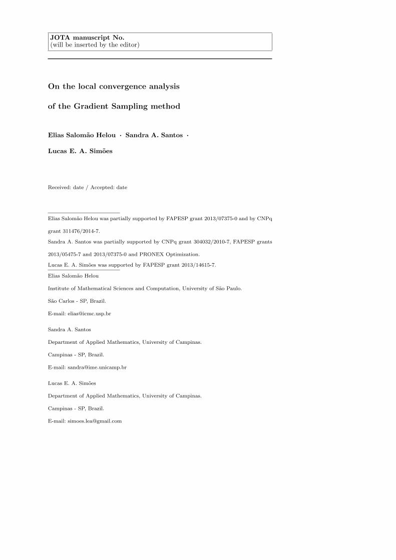
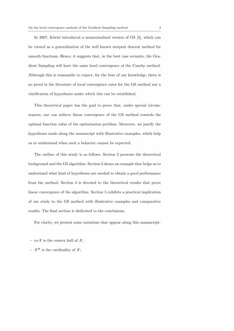
Finally, we present three illustrative examples in order to stress the im-
portance of the relation (14). We have compared the number of iterations
and time (in seconds) versus the distance of the current function value to the
minimum function value f∗ reached along twenty runs. For each example, we
exhibit the median with the first and third quartiles of those runs. The curves
in black stand for the GS method with the parameters suggested by the orig-
inal authors [1], whereas the grey curves represent the same GS method but
now using:
νk = 10−(k+1), ∀k ≥ 0; ε0 = ν0, ε1 = ν1.51 and εk = ν2.25k , ∀k ≥ 2.
All the results were obtained using Matlab and its function quadprog for
addressing the GS subproblem of Step 2.
In Figures 1 and 2, it is possible to see that relation (14) allows the method
to keep behaving with linear rate of convergence until the final iterations, a
characteristic that is not preserved for the usual GS method. Lastly, Figure 3
illustrates the necessity of Assumption 1, since it does not hold for the function
MAXQ.

On the local convergence analysis of the Gradient Sampling method 27
10−14
10−12
10−10
10−8
10−6
10−4
10−2
100
102
104
0 1 2 3 4 5 6 7 8
f(xk)−f∗
Time (seconds)
(a) n = 10
10−14
10−12
10−10
10−8
10−6
10−4
10−2
100
102
104
0 50 100 150 200
f(xk)−f∗
Number of iterations
(b) n = 10
Fig. 1 Results for the nonsmooth convex function Chained CB3 II [9]. It satisfies
dim{U(x∗)} ≥ 1.
10−14
10−12
10−10
10−8
10−6
10−4
10−2
100
102
104
0 5 10 15 20
f(xk)−f∗
Time (seconds)
(a) n = 10
10−14
10−12
10−10
10−8
10−6
10−4
10−2
100
102
104
0 50 100 150 200 250 300 350 400
f(xk)−f∗
Number of iterations
(b) n = 10
Fig. 2 Results for the nonsmooth nonconvex function Chained Crescent I [9]. It satisfies
dim{U(x∗)} ≥ 1.
6 Conclusions
In this manuscript, we have established a linear local convergence result for
the function value sequence generated by the nonnormalized version of the GS
method. Our analysis does not provide any kind of local convergence result
for functions such that V (x∗) = Rn. Moreover, as it is reasonable to expect,
for nonsmooth functions for which dim{U(x∗)} ≥ 1, a good decrease of the
28 Elias Salomao Helou et al.
10−30
10−25
10−20
10−15
10−10
10−5
100
105
0 5 10 15 20 25 30 35 40
f(xk)−f∗
Time (seconds)
(a) n = 5
10−30
10−25
10−20
10−15
10−10
10−5
100
105
0 500 1000 1500 2000 2500 3000 3500
f(xk)−f∗
Number of iterations
(b) n = 5
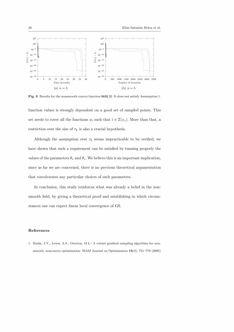
Fig. 3 Results for the nonsmooth convex function MAXQ [9]. It does not satisfy Assumption 1.
function values is strongly dependent on a good set of sampled points. This
set needs to cover all the functions φi such that i ∈ I(x∗). More than that, a
restriction over the size of τk is also a crucial hypothesis.
Although the assumption over τk seems impracticable to be verified, we
have shown that such a requirement can be satisfied by tunning properly the
values of the parameters θν and θε. We believe this is an important implication,
since as far we are concerned, there is no previous theoretical argumentation
that corroborates any particular choices of such parameters.
In conclusion, this study reinforces what was already a belief in the non-
smooth field, by giving a theoretical proof and establishing in which circum-
stances one can expect linear local convergence of GS.
References
1. Burke, J.V., Lewis, A.S., Overton, M.L.: A robust gradient sampling algorithm for non-
smooth, nonconvex optimization. SIAM Journal on Optimization 15(3), 751–779 (2005)

On the local convergence analysis of the Gradient Sampling method 29
2. Burke, J.V., Henrion, D., Lewis, A.S., Overton, M.L.: Stabilization via nonsmooth, non-
convex optimization. IEEE Transactions on Automatic Control 51(11), 1760–1769 (2006)
3. Kiwiel, K.C.: Convergence of the gradient sampling algorithm for nonsmooth nonconvex
optimization. SIAM Journal on Optimization 18(2), 379–388 (2007)
4. Clarke, F.H.: Optimization and nonsmooth analysis, vol. 5. SIAM, Montreal, Canada
(1990)
5. Goldstein, A.A.: Optimization of Lipschitz continuous functions. Mathematical Program-
ming 13(1), 14–22 (1977)
6. Mifflin, R., Sagastizabal, C.: VU-decomposition derivatives for convex max-functions.
In: M. Thera, R. Tichatschke (eds.) Ill-posed Variational Problems and Regularization
Techniques, Lecture Notes in Economics and Mathematical Systems, vol. 477, pp. 167–
186. Springer Berlin Heidelberg (1999)
7. Nocedal, J., Wright, S.: Numerical Optimization. Springer-Verlag, New York (2006)
8. Bonnans, J.F., Gilbert, J.C., Lemarechal, C., Sagastizabal, C.A.: Numerical optimization:
theoretical and practical aspects, 2nd edn. Springer-Verlag Berlin Heidelberg (2006)
9. Skajaa, A.: Limited memory BFGS for nonsmooth optimization. Master’s thesis, Courant
Institute of Mathematical Science, New York University (2010)