U.S. DEPARTMENT OF COMMERCENATIONAL OCEANIC AND ATMOSPHERIC ADMINISTRATION

NATIONAL WEATHER SERVICENATIONAL METEOROLOGICAL CENTER

OFFICE NOTE 69

On the Longitudinal Smoothing of the Tendency Fieldsin the Eight-Layer Hemispheric PE Model (HEMPEP/8)

(A Chronicle)

John D. StackpoleDevelopment Division

JANUARY 1972

The General Problem

In a latitude-longitude coordinate system, with the mathematical polelocated at the geographic pole, the convergence of the meridians (as onemoves northward) brings the grid points sufficiently close together thatthe CFL linear stability criterion (1) Ax/At > c (Ax = r cos 6A) becomesimpossible to satisfy without an inordinately short time step At. Anumber of solutions to this problem have been proposed which fall into twobroad categories: 1) one may simply delete grid points from the grid asone moves north (Kurihara, (2)) such as to maintain an approximate constancyto the geographic distance between grid points or 2) one may perform somesort of smoothing to either the data fields or the tendency fields to suppressthe growth of CFL unstable waves.

There are rather severe difficulties associated with the solutions ofcategory 1 which have been well explored (Shuman (3), Dey (4)); it is someof the less explored problems associated with solution category 2 to whichI wish to turn my attention. In particular, we shall investigate some ofthe apparent consequences of the smoothing of the tendency fields by theoriginal method proposed for the Hemispheric eight-layer PE model and offersome possible solutions to the difficulties encountered.

A Digression - Fourier Transforms

The most convenient method of talking about smoothing and its effectsis in terms of Fourier transforms. This is because "smoothing" is moreproperly (at least, in Fourier type terms) referred to as convolution. Andthere are all sorts of nice theorems dealing with convolution. (In thisdigression, we shall ignore all those problems that excite mathematicianslike integrability, and convergence, and existence, and limits, and dis-continuities, and pretend that all the needed conditions are met.)

If f(x) g(x) are functions of (nondimensional space) x, F(s) and G(s)

their transforms in frequency space (s=l/x), and convolution is

f(x)gx) E. I u) gx-udu

f(x)*g(x) -f f(u) g(x-u)du

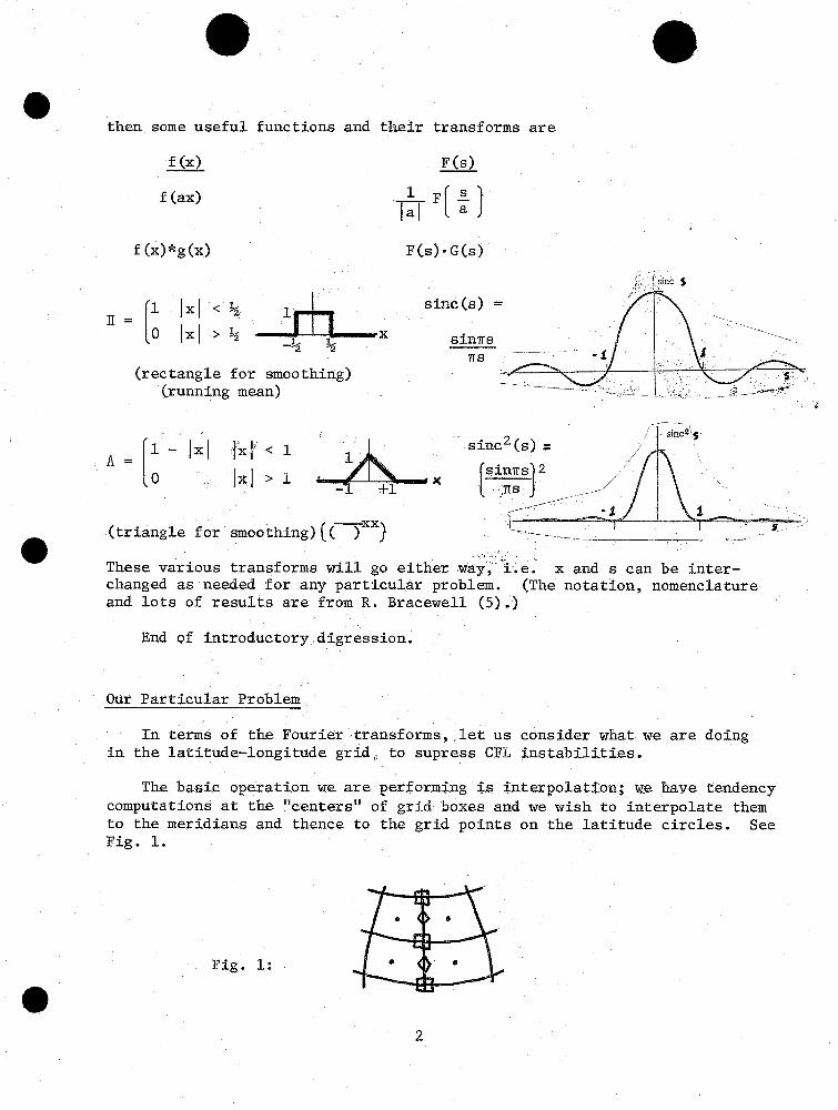
then some useful functions and their transforms are

f(x) F(s)

f(ax) I s ja a

f (x)*g(x)

0~~~ I1 | I < Eta

I o lxI , . I zrW

F(s)-G(s)

sinc(s) =

x sin7rs

(rectangle for smoothing)(running mean)

A=[1 -xi < 1 10/to A i lx > i(O~ ~~ -1; +rl

·~~2 ' ~/ sincZssinc (S) = ( '

Id X [-- :''in!rs I 2/ rens2"I \'" t.<Tj~~-

(triangle for smoothing)(( } -- ... . .

These various transforms will go either way, i.e. x and s can be inter-changed as needed for any particular problem. (The notation, nomenclatureand lots of results are from R. Bracewell (5).)

End of introductory digression.

Our Particular Problem

In terms of the Fourier transforms, let us consider what we are doingin the latitude-longitude grid, to supress CFL instabilities.

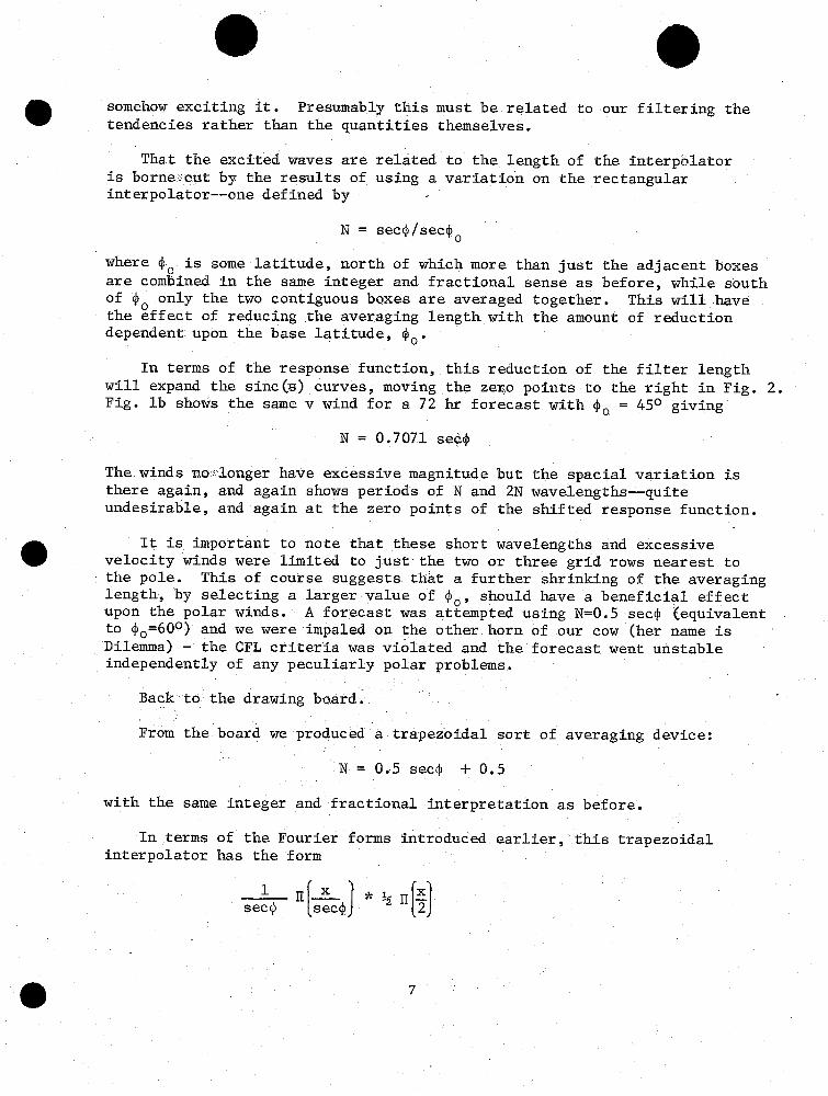
The basic operation we are performing is interpolation; we have tendencycomputations at the "centerst" of grid boxes and we wish to interpolate themto the meridians and thence to the grid points on the latitude circles. SeeFig. 1.

Fig. 1:

2

_ .

The tendency values are at the points - we interpolate in longitude to theO points and then in latitude to the points. (Interpolation is just avariation on convolution--no trouble there.)

No particular difficulty accrues to the interpolation in the north-south direction--the grid rows retain the same geographic separation every-where on the globe and the analog to a (-Y operation, convolution of thedata with a ½ii() function, seems sufficient to perform the interpolation.We have assumed that the grid row separation has the value unity--we shallmaintain this assumption--the grid column separation therefore has the valuecos c (4= latitude) and that is the crux of our problem.

In order to maintain CFL stability, we wish to increase the east-westaveraging in terms of grid points such that the effective averaging length(not precisely defined as yet) remains the same with respect to the earthi.e. a grid averaging length which varies as sec 4.

The first of a number of interpolators tested was of the form

1~~~~~~~~~~~~~~~~~~~~~~~~~~~

2 sec q [ 2sec:

i.e. a rectangular function which expands as the secant of latitude.

Fig. 2 is a collection of sketches of its response function at various

latitudes as a function of grid length frequency. A value of s of 0.5represents the two grid length wave, which wave has a shorter geometriclength the greater the latitude, and is also the highest frequency waveresolvable by the grid. In this respect, the portions of the curves tothe right of s = 0.5 are mythical--there are no waves out there to befiltered.

But consider what is happening to the left of the cutoff frequency--at the equator the shortest (in geometric terms) resolvable wave is the2 grid length wave, a wave length of approximately 560 km. Presumably, wewish to suppress waves shorter than this length further north even thoughsuch shorter waves became resolvableas the meridians converge. This wave,the equatorial equivalent two grid wave, falls at the first zero on thesinc (2s.sec(q)) curves of Fig. 2. It is immediately evident that waves of

frequencies higher than the equatorial equivalent two-grid wave are notparticularly well-filtered by the rectangular interpolator especially nearthe pole. Presumably, such higher than desirable frequencies will begenerated by the nonlinearities of the equations--what will become of themis a matter of experiment.

3

0 IUJF 10 X 10 TO l/2 INCH 46 13207 X 'tO INCHES IADE IN U. S. A.

KEUFFEL & ESSER CO.0 0

I

h ad 3 ,J .5 S :7 . II .H:i

i $FEE

:, a

*

Another way to write down and compute the form of the interpolatingfunction is to consider a number N: its integer part shall be the numberof tendency values (in the boxes) given unit weight on either side of themeridian being averaged to and its fractional part shall be the weightgiven the next tendency value out. This is a rectangular interpolator withwings.

The simplest one is: N = secO.

At the equator, this average combines the two adjacent boxes, at 60°N thefour neighboring boxes with equal weight, and at 86.25° N = 15.29, i.e.the interpolator reaches out some 32 grid lengths (80° longitude over allat the northernmost latitude at which this averaging is performed. Thirtytendencies receive equal unit weight--the two ultimate ones weights of0.29 each. A geometric interpretation of the interpolator is

A

o 0

- 1 I: 1- 1 * I * I * 1 1 *1 I1

and boxes fully under the bar X get equal weight--those partially coveredget that fraction of coverage.

As one might have anticipated from the discussion of the spectralresponse, difficulties were encountered in the use of the rectangularinterpolator. But what was surprising was the nature of the problem andthe dilemma that it introduced.

A series of forecasts using a 2.5° barotropic model illustrates theproblem. Fig. 3 shows the 72 hr forecast of the v component of the windat the grid row just south of the pole for three different interpolators.For the first of these (Fig. la), the N=l.sec~ rectangular interpolatorpreviously introduced, it is evident that there is trouble - 300 m/s windsseem a bit excessive. However, somewhat more interesting is the appearancein the data of two periodicities--one with a wave length of N and anotherwith wave length 2N grid lengths. It seems that the long reach of theinterpolator somehow excites waves in the forecasts (after sufficient time--the 48 hr forecasts show none such at all) with a wave length equal to theinterpolating length and at least its first harmonic.

What is particularly curious is that these two periodicities fall asnearly as one can tell at the first two zeros of the response function--the filtering interpolator should be eliminating this wave and yet it is

*O u ~~~~~~~~~~~5

w --i

-- ------ --- --~ +H

---- ------- ~~~~~~~~~~~'

I L-Z) I

--- ------- ~~~~~~~~~~~~~~~~~~~~~~~~~~~~~~~~~~~~-- ; 1

o~~~~~~~~~~~~ii~~~~~~~~~~~~~~~~~~ -~~~-- -----I I - III~~~~~~~~~~~~~4 +R

LAJ - - --- --

---- -- ---- ~ ~ ~ ~ ~ ~ ~ ~ ~ ~ ~ ~ ~ ~ ~ ~ ~ ~ ~ ~ ~~~~~~~~~~~~~~~

- - - - - - - - - - - - - - - --I -- - - I

- I I '~~~~~~~~~~~~~~~~~~~~ - -- - -

Li~ ~ L~ 4 ~iv S) tD~to/) kf 'c f-, 1b () iT

somehow exciting it. Presumably this must be related to our filtering thetendencies rather than the quantities themselves.

That the excited waves are related to the length of the interpolatoris borne out by the results of using a variation on the rectangularinterpolator--one defined by

N = sec~/seco

where 4o is some latitude, north of which more than just the adjacent boxesare combined in the same integer and fractional sense as before, while southof 0 only the two contiguous boxes are averaged together. This will havethe effect of reducing the averaging length with the amount of reductiondependent upon the base latitude, 40.

In terms of the response function, this reduction of the filter lengthwill expand the sinc(s) curves, moving the zero points to the right in Fig. 2.Fig. lb shows the same v wind for a 72 hr forecast with o = 450 giving

N = 0.7071 sec4

The winds no::longer have excessive magnitude but the spacial variation isthere again, and again shows periods of N and 2N wavelengths-quiteundesirable, and again at the zero points of the shifted response function.

It is important to note that these short wavelengths and excessivevelocity winds were limited to just the two or three grid rows nearest tothe pole. This of course suggests that a further shrinking of the averaginglength, by selecting a larger value of 0o, should have a beneficial effectupon the polar winds. A forecast was attempted using N=0.5 seco (equivalentto Oo=600) and we were impaled on the other horn of our cow (her name isDilemma) - the CFL criteria was violated and the forecast went unstableindependently of any peculiarly polar problems.

Back to the drawing board.

From the board we produced a trapezoidal sort of averaging device:

N = 0.5 seco + 0.5

with the same integer and fractional interpretation as before.

In terms of the Fourier forms introduced earlier, this trapezoidalinterpolator has the form

1 sec * ½e

7

i.e. the convolution of a rectangle function which expands as the secant oflatitude with a simple two point rectangle function. The effect of theconvolution is to change the interpolator function from this

to this

' e n = sec - 2

putting triangle wings on the original rectangle. Note that the rectangleportion of the trapezoid (the portion that expands) is half the width of therectangle previously used. This is the same width as the N=0.5 sec4interpolator that did not suppress the CFL instabilities--however, as weshall see the addition of the trapezoidal sides allowed for a successfulforecast. But before that, let's take a look at the spectral characteristicsof our compound interpolator.

Since convolution in one domain is equivalent to multiplication in theother, we can use our rules from our digression on transforms to immediatelywrite down the spectral character of the interpolator as

sincrs sec(q)} · sinc(2 s)

Fig. 4 contains some sketches of the responses for selected values of ~.I have not bothered to extend the curves beyond the cutoff frequency which,please note, has been approached by the zeros of the response function--thisis a simple reflection of diminishing the length of the interpolator: theresponse function widens in the frequency domain. We can note in the figurein comparison to Fig. 2 that the responses at the higher latitudes are littlechanged other than being shifted to higher frequencies while the responsesfrom 60°S are appreciably altered--principally by the elimination of thenegative lobe.

The very encouraging result of the 72 hr forecast with the trapezoidalinterpolator is the third portion of Fig. 1: no trace of 8 or 16 grid length

waves are to be seen and the wind values are quite proper. That thisimprovement is due to the form of the interpolator and not due to the slightlysmaller extreme averaging length (N=8.15 vs N=10.7 for the 0.7071 sec% case)is evidenced by a run made with N=0.543 secf - the ~o selected so that themaximum, near polar, averaging length would be the same, 8.15, as the

8

_E, 1. X 10 T. 1',2 INCHI 46 1320_l " 7 X 10 INCHES MADE 114 U..A.

KEUFFEL & ESSER CO. 0

o 0 . I . .i,1 ,g' !s --pE -"5/, rB # 4 I

w 4WOtrapezoidal interpolation has there. This run succumbed to CFL instabilitieswithin the 6th hour of its forecast. The explanation is simple - thetrapezoidal interpolator is wider farther south than the rectangular one andthe width is needed.

A certain degree of enthusiasm might well be justified by the resultsof this series of experiments--and it would seem we are comfortablypositioned on Dilemma's head, firmly grasping her horns, forging ahead.Dilemma promptly grew a third horn (labeled "Baroclinic Model") midwaybetween the others.

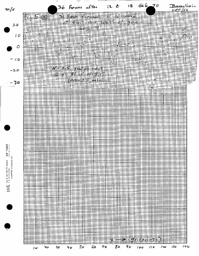
Inforporating the trapezoidal interpolator into the eight-layer modeldid not prevent the model from blowing up (numbers too large for the computer,etc.) after all of two hours of forecast time. The instabilities were mostpronounced near the pole. As an uneconomic means of getting something out,the time step was reduced to 7.5 min with the result that the forecastsurvived to about hour 37 with the severe instabilities first appearing nearthe pole. Fig. 5 illustrates the situation with the near polar v windcomponent in the topmost layer of the model at hour 36. Although 8.15 or16.3 grid length waves are not as clear cut'as were the average-excitedwaves with the rectangle smoother in the barotropic model, things are mostassuredly not what they ought to be. Why?

About all that one can do is speculate that the additional layers affordmore degrees of freedom in the model (vis a vis the barotropic well-behavedcase) and hence more modes of response to the filter. And the numerics pro-.ceed to respond. Badly. Dilemma is still tossing her head about.

Back to the drawing board.

And off the board we pull a triangular averager with the form

xw = 1. - L sec() x = ½, 1½, 2½ < L sect

x is in grid length units, the values x takes on being the location of thetendencies and the L in the denominator allows us to make the triangle aswide or narrow as we please.

This interpolator was tested first on the barotropic model (with L = 1)and as might have been anticipated, worked just fine - there was no trace ofinterpolator excited polar waves.

Not without some anxiety, the triangular interpolator was introducedinto the baroclinic model (with L=1). With a 10 min time step, the model

9

~~~~~~~~ ~ ~ ~ ~~iiiiAtIi 11-'i-ttt-11Ii1r--r

(V~ ~~~H +i+1++-H H

- w ~ ~ ~ ~ ~ - - - - - - - -

ow J

3-U I - --- - ----- -

C- D ~ ~ ~ ~ ~ ~ ~ -- -- - -

U~~~~~~~

ILAJI~~~~~~~~~~~~

.36 rw sw" I -L- L- I fs -4:e-- v�Allg4,c.

/ 2-dw 12L), 16? D-

succumbed to linear instabilities before the third hour was reached but theywere in no way polar related.

Upon reflection, this was not so surprising. Fig. 6 illustrates thespectral response function of the triangular interpolator

W = Lsec A[L sec

which is

R = sinc 2 (L secO s)

for L=l and the same selection of latitude values used previously. Comparisonof Fig. 6 with Fig; 2 and Fig. 4 suggests that we should better use atriangular interpolator with L=2. This will shrink the response functions,moving their zero points to the left by a factor of 0.5. Also the Fouriersketches show that the spectral response of a triangular filter is suchthat the triangle must be twice as wide as a rectange in order for tharesponse function to drop to its first zero at the same frequency as therectangular response function. An earlier run of the baroclinic model witha rectangular interpolator with half width equal to sec(4) had run to 42hours with 10 min time steps before blowing out at the pole. This wassufficiently encouraging to try the triangle again with L=2.

In spite of the near polar reach of the triangle being some 62 gridpoints (155° of longitude), and using a 10 min time step, no polar problemswere encountered at all--the forecast ran just fine to 48 hours. See Fig. 7for the near polar v wind component at 48 hours.

It would seem that the difficulties with the averager-interpolator havebeen resolved and we can go on to meteorology.

The solution was not free--the use of the variable weight interpolator,i.e. the triangle, increased the running time of the model some 40 to 50%--these problems will be neglected for the time being. At least the model runs.

An engineering approach to helping the running time is to reduce thetriangle width--a run with L=l.5 ran some 10% faster than L=2.0 and behavedjust as well.

As to why the triangular interpolator worked where the others didn't,about all one can speculate is that the absence of negative (phase changing)lobes in the triangle.. 's response function made the difference.

But it works and that's enough for now.

10

L E 7 X 10 INCHES MA46 1320[ -r 7 X I INCHES 1ADE IN U.S.A.

KEUFFEL & ESSER Co.4 0

0 , I ,

.

,3 ,"- , (. , , 7 . F .I /,o

)-5-,) "-D

0

z ~

-

u

x_ 0

;la

x

WU

0

-~ ,,I m

FV L

Z D

-

f m U.

%

k X v &o?-L. Cou ca /Ad~ Il tYLo

References

(1) Courant, Friedrichs & Levy, 1928: Math. Ann., 100: 32-74.

(2) Kurihara, Y., 1965: "Numerical Integration of the Primitive Equationson a Spherical Grid," Mon. Wea. Rev., V. 93, p. 399.

(3) Shuman, F. G., 1970: "On Certain Truncation Errors Associated withSpherical Coordinates," J. App. Met., V. 9, p. 564-570.

(4) Dey, C. H., 1969: "A Note on Forecasting with the Kurihara Grid,"Mon. Wea. Rev., V. 97, p. 597-601.

(5) Bracewell, R., 1965: "The Fourier Transform and its Applications.'"McGraw Hill Book Co.

: