On the Operational Aspects of Measuring Nanoparticle Sizes

nanomaterials

Article

On the Operational Aspects of MeasuringNanoparticle Sizes

Jean-Marie Teulon 1,2,†, Christian Godon 2,3,†, Louis Chantalat 2, Christine Moriscot 4,Julien Cambedouzou 5,‡ , Michael Odorico 2,5, Johann Ravaux 5, Renaud Podor 5 ,Adèle Gerdil 6, Aurélie Habert 6, Nathalie Herlin-Boime 6, Shu-wen W. Chen 7 andJean-Luc Pellequer 1,2,*

1 Univ. Grenoble Alpes, CEA, CNRS, IBS, F-38000 Grenoble, France; [email protected] CEA, iBEB, LIRM, F-30207 Bagnols sur Cèze, France; [email protected] (C.G.);

[email protected] (L.C.); [email protected] (M.O.)3 CEA, BIAM, LBDP, F-13108 Saint Paul lez Durance, France4 Univ. Grenoble Alpes, CNRS, CEA, IBS, F-38000 Grenoble, France; [email protected] Univ. Montpellier, Institut de Chimie Séparative de Marcoule (ICSM), CEA, CNRS, ENSCM,

F-30207 Marcoule, France; [email protected] (J.C.); [email protected] (J.R.);[email protected] (R.P.)

6 UMR3685 CEA-CNRS, NIMBE, LEDNA, CEA Saclay, F-91191 Gif sur Yvette, France;[email protected] (A.G.); [email protected] (A.H.); [email protected] (N.H.-B.)

7 478 rue Cyprien Jullin, F-38470 Vinay, France; [email protected]* Correspondence: [email protected]; Tel.: +33-45742-8756† These authors contributed equally to this work.‡ Present address: IEM, CNRS, ENSCM, Univ. Montpellier, F-34000 Montpellier, France.

Received: 26 November 2018; Accepted: 17 December 2018; Published: 23 December 2018 ��

Abstract: Nanoparticles are defined as elementary particles with a size between 1 and 100 nm forat least 50% (in number). They can be made from natural materials, or manufactured. Due to theirsmall sizes, novel toxicological issues are raised and thus determining the accurate size of thesenanoparticles is a major challenge. In this study, we performed an intercomparison experiment withthe goal to measure sizes of several nanoparticles, in a first step, calibrated beads and monodispersedSiO2 Ludox®, and, in a second step, nanoparticles (NPs) of toxicological interest, such as SilverNM-300 K and PVP-coated Ag NPs, Titanium dioxide A12, P25(Degussa), and E171(A), usingcommonly available laboratory techniques such as transmission electron microscopy, scanningelectron microscopy, small-angle X-ray scattering, dynamic light scattering, wet scanning transmissionelectron microscopy (and its dry state, STEM) and atomic force microscopy. With monomodaldistributed NPs (polystyrene beads and SiO2 Ludox®), all tested techniques provide a global sizevalue amplitude within 25% from each other, whereas on multimodal distributed NPs (Ag andTiO2) the inter-technique variation in size values reaches 300%. Our results highlight several pitfallsof NP size measurements such as operational aspects, which are unexpected consequences in thechoice of experimental protocols. It reinforces the idea that averaging the NP size from differentbiophysical techniques (and experimental protocols) is more robust than focusing on repetitions of asingle technique. Besides, when characterizing a heterogeneous NP in size, a size distribution is moreinformative than a simple average value. This work emphasizes the need for nanotoxicologists (andregulatory agencies) to test a large panel of different techniques before making a choice for the mostappropriate technique(s)/protocol(s) to characterize a peculiar NP.

Keywords: nanoparticles; nanotoxicology; metrology; AFM; TEM; SEM; wet-STEM; SAXS; DLS

Nanomaterials 2019, 9, 18; doi:10.3390/nano9010018 www.mdpi.com/journal/nanomaterials

http://www.mdpi.com/journal/nanomaterials

http://www.mdpi.com

https://orcid.org/0000-0002-8811-5667

https://orcid.org/0000-0002-8103-1743

https://orcid.org/0000-0002-8944-2715

http://dx.doi.org/10.3390/nano9010018

http://www.mdpi.com/journal/nanomaterials

http://www.mdpi.com/2079-4991/9/1/18?type=check_update&version=2

Nanomaterials 2019, 9, 18 2 of 29

1. Introduction

Despite differences in international definitions on nanoparticles (NPs) especially concerningsolubility, aggregation, and distribution threshold, current regulatory agencies consider that aprimary nanomaterial is a nanoparticle (NP) when at least one of its dimensions is in the range1–100 nm [1], values below the diffraction-limited resolution of conventional microscopy. In Europe,the 2011/696/EU commission recommendation states that a product containing primary particles for50% or more of the particles in the number size distribution and one or more external dimension in thesize range 1–100 nm is a nanomaterial [2]. It also states that the 50% threshold is adjustable between 1%and 50% when warranted by specific concerns. The European Joined Research Centre published tworeports on the requirements on measurements for the implementation of the EU commission definitionof the term nanomaterial by listing an ensemble of currently used techniques with pros and cons whenmeasuring fine sizes of nanomaterials [3] and on the application of the commission 2011/696/EUrules [1]. In the latter, a description of difficulties encountered for strictly identifying nanomaterial dueto the number threshold is provided. Growth of the usage of NPs in industry is continuous [4,5] anda comprehensive report has been made by the Royal Society, UK, with 21 recommendations on theapplication of nanotechnology and their impact on health and environment [6].

Based on their chemical nature, NPs are used for instance as mechanical reinforcement additiveswith carbon nanotubes, solar cells, paints, coatings, or sunscreen cosmetics with TiO2; wound dressing,air filters, or toothpastes with Ag; and chemical sensors, hydrogels, or drug delivery with nanolatex [7,8].Uptake of NPs in humans occurs via inhalation, ingestion, or transdermal routes. Toxicology of NPshas been investigated for several decades [9] and the sub-discipline nanotoxicology was first coined in2004 [10]. The currently identified toxicity mechanisms are membrane disruption, protein oxidationgenotoxicity, reactive oxygen species formation, and interruption of energy transduction in cells [8].Concerning NPs, the current paradigm stipulates that at the nano-size (<100 nm in diameter) physicaland chemical properties are different from those of the same material in the bulk (non-nano) form [4].Consequently, there is a growing concern that such NPs possess unexpected toxicological properties.Because smaller and smaller NPs expose more and more atoms at their surfaces, particle toxicologygenerally assumes that an increase in particle surface leads to an increase in toxicity [11].

Assessing the potential toxicity of NPs in biological systems starts with a complete and accurateNP characterization [12]. From a regulatory standpoint, the effect of NPs size was the most extensivelystudied property. Numerous studies claimed a greater toxicity for small NPs [13]. Beyond the case ofone-dimensional nanomaterials such as carbon nanotubes, whose toxicity has intensively been debateddue to their similarity with asbestos fibers [14], many examples can be found concerning more isotropicparticles. Due to their small sizes, it is expected that NPs penetrate easily in tissues and cells. Depositionof carbon NPs (23 nm) accumulate more in asthmatic than normal patients [15]. Small Ag NPs haveincreased hemolytic toxicity compared to observations in presence of large agglomerates of Ag [16].Small size of CdO NPs (22 ± 3 nm) reveals severe bacterial surface damages [17]. High bronchoalveolarinflammation was observed in a group of rats exposed to small TiO2 particles (20 nm in size) [9]compared with large-sized particles (250 nm). Similarly, small TiO2 or SiO2 NPs translocate throughthe Calu-3 monolayer with an increased translocation for the smallest and negatively charged NPs [18].Exposure to SiO2 (15 and 30 nm) exerts toxic effects on HaCaT cells by altering protein expression andthe cellular apoptosis is also greatly increased compared with micro SiO2 (365 nm) [19]. Some recentstudies have found that, even at the nanoscale level, small SiO2 NPs (15 nm) show higher toxicityin Caco-2 cells than larger SiO2 NPs (55 nm) and the observed genotoxic effects are likely mediatedthrough oxidative stress rather than a direct interaction with DNA [20]. In addition, it has beenobserved that SiO2 NPs (70 nm) penetrate the cell nucleus of human epithelial cells [21], whereas smalllatex NP beads (<40 nm) entered epidermal cells after transcutaneous applications on human skin [22],while only neutral, small, and positively charged polysaccharide-based NPs (<60 nm) transcytozed onbrain capillaries of endothelial cells [23].


However, contradictory effects regarding NPs size have been observed in the literature.For instance, it has been observed that small Ni:Fe NPs (10 ± 3 nm) are less toxic than largeparticles (150 ± 50 nm) and that cytotoxicity increases when particles are coated with oleic acids [24];and similarly for small TiO2 NPs (10 nm) versus large NPs (>200 nm) [25]. While 70 nm-sizedSiO2 particles were found to enter into the cell nucleus, it was also observed for NPs of larger size(>200 nm) [21]. Distinct effects of TiO2 and SiO2 have been observed on endothelial cells dependingon cell types, concentrations, and exposure time [26] and similarly for CeO2 (8 and 35 nm) and SiO2

(177 and 315 nm) NPs [27]. The size of NPs has been shown to be an important parameter for thedestabilization of biological membranes but it was found that only large NPs (>100 nm) induced anincreased disruption of membrane domain structures [28].

The terminology “particle size” is likely technique- and application-dependent [29]. For instance,non-microscopy techniques (such as dynamic light scattering, DLS) rely on the extraction of NP sizesusing basic assumptions such as sphericity, and all techniques struggle at very low or very highNP concentrations. Microscopy-based techniques suffer from severe artifacts induced by dryingmainly due to the retraction of the liquid meniscus either disrupting or promoting agglomerates.In addition, electron microscopy needs to maintain an electron dose below 1 MGy/s to avoidunwanted alterations [29]. A recent review presents advantages and disadvantages of microscopyand non-microscopy techniques to determine NPs size [29]. Likely, the oldest indirect techniqueto determine NPs size for powders is the Brunauer–Emmett–Teller (BET) method [30]. The mostfrequently used techniques for determining NP sizes are the Scanning or Transmission electronmicroscopies (SEM or TEM, respectively) and light scattering (e.g., dynamic light scattering, DLS).Additional techniques are also often used such as atomic force microscopy (AFM), small-angle X-rayscattering (SAXS), or nanoparticle tracking analysis (NTA). A recent technique has appeared inNPs size determination (field-flow fractionation, FFF and its related variants), but it is rather aseparation technique since the NP size must be determined by additional modules such as DLS ormulti-angle light scattering (MALS). Finally, standard methods such as UV-vis absorption, fluorescence,gravimetry, mass spectrometry (especially ICP-MS), and others are also used for determining NPssizes [31]. Principles of biophysical methods used to characterize NPs have been described previouslyin detail [32,33].

To refine the biophysical methodologies for fine characterization of NPs size, several inter-laboratoryor inter-technique comparisons have been performed [31,32,34–42]. These comparisons involvedeither several groups with the same technique, several groups with different techniques on a singletype of NP, or several groups with different techniques and different types of NP. All the testedmethods of size analysis are subject to a variety of pitfalls [36] and it has been concluded that theanalyst should be knowledgeable and skilled in the technique employed. For instance, large variationswere observed among DLS, AFM, NTA, and fluorescence correlation spectroscopy [40], where up tofive times variations in NP sizes were observed between DLS and TEM [35]. It was found that thetechniques most prone to artifacts were those that are the most frequently used in the literature: TEMfollowing air drying of a sample and DLS [36]. A common conclusion from these comparisons is thatthe source of the irreproducible results is the heterogeneity in sample preparation [39] and propersample deposition greatly improves the analysis of the NP sizes [41]. The agglomeration of NPs insolution is often observed and sonication only reduces it and rarely leads to separation of primaryparticles [35] and sometimes ultrasonication was even observed to further increase variability in NP sizedetermination [38]. It has been suggested that the lack of standardization in the application of ultrasonictreatments across laboratories is a major cause of variability in NP suspension characteristics [43]although several groups are working on NP dispersion by studying the effect of ionic strength, pH,and particle surface chemistry [44] or various dispersion methods [45]. These studies highlight theneed to substantiate characterization from manufacturers, the need to form multidisciplinary teamsperforming measurements as close to the biological action as possible, and the need to provide amaximum transparency in reporting size and size distributions in the literature.


As concluded by previous inter-laboratory comparison experiments, the need to bettercharacterize NPs size remains of major importance. The inter-laboratory experiment presentedin this work aimed at identifying which and when a methodology is best suited for NP sizecharacterization. The rationale of our project was to first test each technique using calibratednanomaterials and monodispersed solutions of NPs to evaluate potential bias of each techniquetoward small sized NPs. To our knowledge, this work is the first comparison that includes thewet-STEM (wSTEM) technique for NP size determination. The aim of the project was also to analyze“realistic” NPs of nanotoxicology interest (Silver and Titanium oxides [46,47]) with an “as is” principlemeaning without standardized protocol. Our project relied on experts in biophysical techniques(electron and atomic force microscopies, small angle X-ray scattering, and dynamic light scattering).It was requested to perform measurements of the size of NPs using classical laboratory standardprotocols and methodologies. The project had three phases: first, provide measurements and theircomparison on standard nanomaterials (standard polystyrene beads); second, provide measurementson monodispersed NPs (silica, Ludox) that could be characterized by all participating techniques; and,third, provide measurements on Ag and TiO2 NPs, which are of major concerns in nanotoxicology.A secondary goal was to provide clear indications of which technique(s) is (are) best suited forwhich NPs.

2. Materials and Methods

2.1. Nanoparticles

Calibrated polystyrene nanoparticles (3000 series Nanosphere™ 20 nm size standard, batch42376, Thermo Scientific, Fremont, CA, USA) were given as a suspension; the nominal diameter was22 ± 2 nm (using photon correlation spectroscopy measurements according to NIST). Colloidal silicananoparticles (Ludox) in suspension were obtained from Sigma-Aldrich (Saint Louis, MO, USA):Ludox®SM-30 (Ref 420794-1L, batch MKBL2470V), Ludox®HS-40 (Ref 420816-1L, batch BCBJ2528V),and Ludox®TM-50 (Ref 420778-1L, batch MKBP2322V). A Ludox®technical literature document fromthe previous manufacturer (E.I. Du Pont de Nemours, Wilmington, DE, USA) provides approximatesizes for SM-30, HS-40, and TM-50 that are ~7 nm, ~12 nm, and ~22 nm, respectively; a recent documentfrom the current manufacturer (Grace, Columbia, MD, USA) reproduces these approximate valueswithout providing technical details of their origin. Consequently, these sizes were not considered inour study, and the Ludox®particle sizes were considered unknown. NPs of TiO2 (P25, Degussa, Essen,Germany) were provided as powders with a primary particle size estimated around 21 nm [48] or23 ± 10 nm [49]. It should be emphasized that P25 NPs used in this study were obtained several yearsago from Degussa, which may not reflect the modern version of P25 from Evonik. TiO2 food additiveE171 (batch A) are those used previously [50] while TiO2 A12 was synthesized in the NIMBE laboratoryto avoid any uncontrolled additives. NPs of silver NM-300K were provided as suspensions by theJoint Research Center (JRC, Ispra, Italy) as a performance standard [51] and were kept in the dark at4 ◦C. Using exclusively electron microscopy, it was found at JRC that NM-300K has an average size of15 nm with 99% of particles having a size <20 nm and a second small population of NM-300K around5 nm has also been observed [51]. Silver NPs with dispersion agent of polyvinylpyrrolidone (Ag PVP)were purchased from Sigma (758329). They are given at a size <100 nm by the manufacturer and a sizeof 59 ± 18 nm was previously obtained with TEM [47]. Detailed instrumentations are shown belowwith an indication of their geographical origin (GRE for Grenoble, MAR for Marcoule, and SAC forSaclay) since similar techniques have been used in different locations. When needed, the geographicalkeyword is added to the name of the technique on figures and tables.

2.2. AFM Measurements (GRE)

Multimode III and multimode 8 with a Nanoscope V controller (Bruker, Santa Barbara, CA, USA)were used. Tapping mode or PeakForce tapping mode were used in ambient condition (air) at room


temperature (24 ◦C). Nanoparticles were deposited on freshly cleaved mica or highly-oriented pyrolyticgraphite (Bruker, Santa Barbara, CA, USA). Cantilevers used for tapping mode were Sn-doped siliconMulti40 (MPP-22200, nominal k = 0.9 N/m, f0 = 54 kHz, Bruker, Santa Barbara, CA, USA), RFESP(MPP-21100, k = 3 N/m, f0 = 69–93 kHz, Bruker, Santa Barbara, CA, USA), and RTESP (MPP-11100,k = 20–80 N/m, f0 = 287–325 kHz, Bruker, Santa Barbara, CA, USA), whereas, for PeakForce tapping,silicon nitride lever with a silicon tip was used (SNL: A, k = 0.35 N/m, f0 = 50–80 kHz; B, k = 0.12 N/m,f0 = 16–28 kHz; C, k = 0.24 N/m, f0 = 40–75 kHz; D, k = 0.06 N/m, f0 = 12–24 kHz). Typical AFMimaging condition was: scan rate of 1 Hz, between 512 and 2048 pixels on 512 to 2048 lines, scan sizeranging from 1 to 10 µm and optimal measurements were obtained with a scan size of 1 µm with1024 × 1024 pixels. In tapping mode, set-point was set to the minimum necessary for imaging, whereas,in peakforce tapping mode, the automated ScanAsyst mode was used.

Image processing was performed in Gwyddion [52], stripe line removal was performed withDeStripe [53], and image enhancements were performed using home-made tools [54,55]. In brief,raw AFM images were flattened using a first-order plan fit. Further line flattening was performedusing leveling tools of Gwyddion. When necessary, a mask was created using Gwyddion to selectnanoparticles and to exclude those for line flattening.

For spherical nanoparticles, NP height was measured using a horizontal profile section withtwo different approaches: for an isolated single NP, the distance between the background and themax height of the profile was measured; for assembled NP, the distance between the max height ofthe first and the last NP divided by the number of NPs was measured. Thus, for a spherical or apseudo-spherical NP, height values are attributed to its diameter.

2.3. TEM Measurements (GRE)

Images were taken under low dose conditions (20 e−/ Å2) with a FEI T12 electron microscope(FEI, Hillsboro, OR, USA) at 120 kV using an ORIUS SC1000 camera (Gatan, Inc., Pleasanton, CA,USA). Samples were prepared according to two protocols: TEM1, the carbon flotation technique [56,57]or, TEM2, directly deposited on carbon-coated grid (S160-4 grids, Agar Scientific Ltd, Stansted, UK).For the flotation technique, 4 µL of samples were injected to the clean side of carbon protected by a micasurface; the carbon was separated from mica by floating on a water drop; and a grid was placed on topof the carbon film, which was subsequently air-dried. The substrate carbon-coated mica was producedby evaporation of a carbon in an Emitech K950X carbon coater (QUORUM Technologie Ltd., Asford,UK). For the carbon-coated technique, samples were directly deposited on the carbon-coated grid,the excess of sample was first removed by blotting with a filter paper and then air-dried. Instrumentcalibration was performed during regular maintenance from the manufacturer. Raw dm3 images(4008 × 2672 px) were analyzed with Gwyddion using cross-section profiles.

2.4. TEM Measurements (SAC)

Images were obtained using a Philips CM12 microscope at 120 kV. Samples were prepared bydifferent protocols depending on whether they come as a power or suspension. For powders, they weredispersed by ultrasonication in acetone or ethanol. The suspensions were used as delivered or after astep of dispersion followed by vortex agitation. In both cases, a drop was deposited on a grid, excesssample was removed with a filter paper and the sample was left for drying under air a few minutes.EM grids were “Lacey Carbon (S166-3H)” or “carbon films (S160-H)” purchased from Agar. The Laceycarbon grids were preferred in the case of agglomerated samples such as TiO2-P25 or TiO2-A12. All theimages obtained from TEM were analyzed using the ImageJ software (version 1.51, NIH, Bethesda,MD, USA) [58] and the line measurement tool. Calibration was regularly checked using standard grids.

2.5. Wet-STEM (wSTEM, MAR)

A Quanta 200 FEG Environmental Scanning Electron Microscope (ESEM) provided by FEI Company(Eindhoven, The Netherlands) equipped with a field electron gun was used to perform the sample


observations. Calibration of the microscope was performed with a standard grid (MRS3, Gellermicroanal. Lab, Topsfield, MA, USA). The Wet-STEM (Scanning Transmission Electron Microscope)is a specific stage that is attached to the ESEM. It allows the direct observation of nanoparticles that aredispersed in an aqueous solution [59]. The observation conditions were: acceleration voltage = 30 kV,working distance = 7 mm, temperature = 2 ◦C, and water vapor pressure =706 Pa. Particularprecautions must be taken not to dry the sample during the pumping in the ESEM chamber. First,a 20 µL drop of the solution to be observed is deposited onto a holey carbon grid. Then, a pumpingsequence is programed to replace progressively the air present in the chamber by the expected pressureof water vapor. When this limit was reached, the water vapor in the ESEM chamber was in equilibriumwith the liquid sample where the temperature was 2 ◦C according to the water phase diagram.Thus, the sample must be thinned sufficiently to be transparent to the electron beam to observe thenanoparticles directly in the liquid layer. This was achieved by slightly decreasing the gas pressure inthe chamber by a few tens of Pa. This yielded the controlled vaporization of water, and a thinningof the sample thickness. When the transparency to the electron beam was obtained, the gas pressurewas kept at 706 Pa, the exact pressure necessary to maintain the equilibrium between the liquid andgaseous phases. Sample observation was preferentially performed through the holes of the holey grid.Indeed, within holes, nanoparticles were expected to remain within the liquid without any contact ofthe particles with the carbon layer. Mobility of nanoparticles also indicates a lack of contact with thecarbon layer. One main limit of this technique was that the thinning of the sample was obtained byevaporating a part of the liquid phase. This yielded an increase of the nanoparticle concentration inthe sample. To overcome this difficulty, the sample was first diluted with pure water (500–1000 times)before to be concentrated approximately to the initial concentration during the thinning of the liquidlayer. When the sample was ready to be observed, i.e., when the nanoparticles were in the aqueousphase, images were continuously recorded with a scanning frequency ranging from 4 to 60 images perminute, depending on the motion of the nanoparticles. Several zones of the sample were observedsuccessively to show the reproducibility of the observations. Size measurements were performed withFiji [60].

2.6. STEM-in-SEM (STEM, MAR)

After being observed in the Wet-STEM mode, the sample was dried under vacuum to be observedwith STEM-in-SEM mode. Dark field and bright field images of the nanoparticles initially dispersed inthe liquid and then stuck on the carbon film of the holey carbon grid could be recorded with a 1 nmresolution. The acceleration voltage was 30 kV.

2.7. SEM (MAR)

Samples were deposited on a carbon stub and dried before introduction in the SEM chamber. Imageswere recorded using an acceleration voltage of 20 or 30 kV. Sample size measurements were performedusing Fiji Software (version 1.49, NIH, Bethesda, MD, USA). The size measurements were calibrated byusing both a calibration grid (Geller reference standard MRS-3XYZ with mount serial No. R30-147) for theSEM mode and a 204 nm latex spheres (202/197 nm and 205/201 nm) for the STEM mode.

2.8. SEM (SAC)

SEM images were obtained with a Carl Zeiss “Ultra 55”. The samples were deposited on a grid(same preparation as TEM (SAC) or directly on an adhesive membrane.

2.9. Small-Angle X-Ray Scattering (SAXS, MAR)

SAXS experiments were performed on a set-up operating in transmission geometry. A Mo anodeassociated to a Fox2D multi-shell mirror (XENOCS) delivered a collimated beam of wavelength 0.710 Å.Two sets of scatterless slits [61] delimited the beam to a square section of side length 0.8 mm. A MAR345imaging plate detector allowed simultaneously recording scattering vectors q ranging from 0.25 nm−1


to 25 nm−1, meaning that distances up to 25 nm could be probed with this set-up. Samples were placedin glass capillaries of diameter 2 mm. Absolute intensities were obtained by measuring a calibrationsample of high-density polyethylene (Goodfellow, Huntingdon, UK) for which the absolute scatteringwas already determined.

SAXS measurements on Ludox samples were carried out after a factor 100 dilution in water. This wasdone to ensure a dilute regime compatible with the observation of typical form factors of the nanoparticles,and to minimize the structure factor contribution arising from nanoparticle interactions. Calculationsof monodisperse spherical form factors were made using the SASFit [62] software and were comparedwith experimental data. The diameter refinement was performed to obtain the best agreement withexperimental data, in particular regarding the position of intensity minima and maxima. Reliability rangescorresponding to acceptable sphere diameters were estimated for each sample.

2.10. Dynamic Light Scattering (DLS, SAC)

For samples purchased as suspensions, DLS measurements were directly performed on a Horibananoparticle analyzer SZ 100. Before any measurement, the calibration is checked with the Nanospherestandard. If needed, concentration was further adapted to allow a proper measurement. For example,for the measurement of nanosphere standard, 2–3 drops of suspension were mixed with pure water.When samples were powders, they were dispersed in water at a temperature regulated at 18 ◦C for20 min (2 s on, 2 s off) at 30% power, using an ultrasonic cuphorn. NP average sizes and standarddeviations were provided by the analyzer software.

2.11. Analysis of Particle Sizes

For most techniques, the size of nanoparticles (NPs) represents their diameter, except forAFM, in which size usually represents the height. In this study, all NPs used, except TiO2 E171,are pseudo-spherical and thus the height and diameter values of the NPs are comparable. To simplifythe text, we only use the term “size” to represent the equivalent diameter or height of NPs; valuesare given as means ± standard deviations (SD) in nm for a given technique, whereas global averagesare given as means of each technique ± standard error of the mean (SEM) in nm. The amplitudepercentage variation is the ratio between the difference of the largest and smallest values over theglobal mean. Normality tests (D’Agostino–Pearson omnibus and Shapiro–Wilk) were performedwithin GraphPad Prism 5.0 with an alpha threshold of 0.05.

3. Results

The main theme of this intercomparison was to perform measurements at local laboratory facilitiesusing daily used in-house protocols. Thus, no specific measurement protocol was designed as usuallyfound in classical metrology study [41] and detailed uncertainties were not requested [63]. The goal wasto perform experiments as close as possible to day-to-day practice so that interpretation of results couldhelp us to present practical guidelines for measuring nanoparticle sizes at local facilities. The experimentwas divided in three steps: (1) use available techniques to perform measurement on a standard system(polystyrene beads) for which the size was certified; (2) run experiments will all the available techniqueson silicate NPs (Ludox®) which are homogeneous solutions but of unknown size; and (3) run experimentson two toxicology-important nanoparticle families: silver and titanium dioxide.

3.1. Size Measurement of a Standard

The nanosphere standard polystyrene particles (called PS22) were certified at 22 ± 2 nm diameterby the manufacturer (using DLS). Only four out of the six biophysical techniques were able to providemeasurements. According to the limitation of local experimental set-ups, no data were obtainedwith SAXS and wet-STEM. SAXS could not provide a determination of the NP diameter due the toosmall electronic contrast between PS22 and water. The signal-to-noise ratio therefore remained too


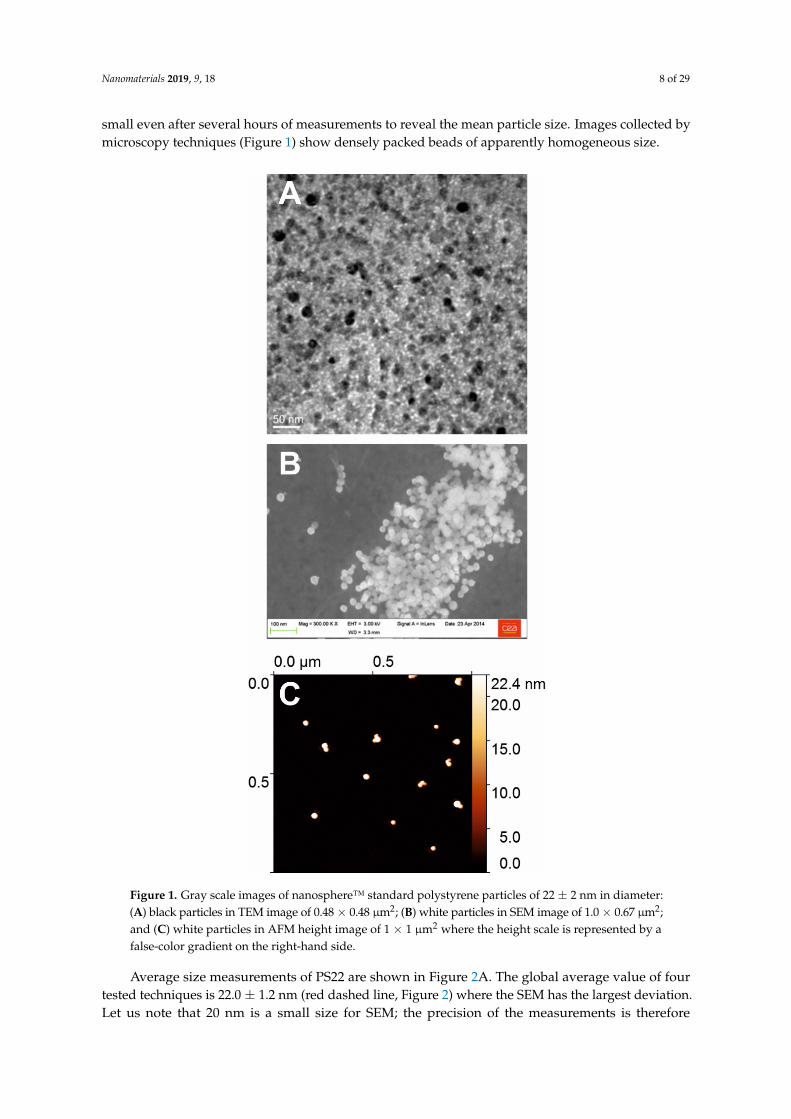
small even after several hours of measurements to reveal the mean particle size. Images collected bymicroscopy techniques (Figure 1) show densely packed beads of apparently homogeneous size.Nanomaterials 2018, 8, x FOR PEER REVIEW 5 of 29

Figure 1. Gray scale images of nanosphere™ standard polystyrene particles of 22 ± 2 nm in diameter: (A) black particles in TEM image of 0.48 × 0.48 µm²; (B) white particles in SEM image of 1.0 × 0.67 µm²; and (C) white particles in AFM height image of 1 × 1 µm² where the height scale is represented by a false-color gradient on the right-hand side.

Average size measurements of PS22 are shown in Figure 2A. The global average value of four tested techniques is 22.0 ± 1.2 nm (red dashed line, Figure 2) where the SEM has the largest deviation. Let us note that 20 nm is a small size for SEM; the precision of the measurements is therefore questionable. Surprisingly, average size of PS22 (19.8 nm) determined by TEM is quite below the reference value, although PS22 size is within the TEM standard deviation. Concerning TEM as well as SEM, the contrast of PS22 NPs was rather poor and may explain the noted over/underestimation of the size. Interestingly, the average value of all the tested techniques is much closer to the reference value than most of individual techniques.

Figure 1. Gray scale images of nanosphere™ standard polystyrene particles of 22 ± 2 nm in diameter:(A) black particles in TEM image of 0.48 × 0.48 µm2; (B) white particles in SEM image of 1.0 × 0.67 µm2;and (C) white particles in AFM height image of 1 × 1 µm2 where the height scale is represented by afalse-color gradient on the right-hand side.

Average size measurements of PS22 are shown in Figure 2A. The global average value of fourtested techniques is 22.0 ± 1.2 nm (red dashed line, Figure 2) where the SEM has the largest deviation.Let us note that 20 nm is a small size for SEM; the precision of the measurements is therefore


questionable. Surprisingly, average size of PS22 (19.8 nm) determined by TEM is quite below thereference value, although PS22 size is within the TEM standard deviation. Concerning TEM as well asSEM, the contrast of PS22 NPs was rather poor and may explain the noted over/underestimation ofthe size. Interestingly, the average value of all the tested techniques is much closer to the referencevalue than most of individual techniques.Nanomaterials 2018, 8, x FOR PEER REVIEW 6 of 29

Figure 2. Size measurement of nanosphere standard particles (PS22) given at a reference diameter of 22 nm (thick red lines) and a standard deviation of ±2 nm (dotted red lines). N represents the number of measurements obtained in each method. (A) Measures were performed with Dynamic Light Scattering (DLS), Scanning Electron Microscopy (SEM) in Saclay (SAC), Transmission Electron Microscopy (TEM), and Atomic Force Microscopy (AFM). The red dashed line corresponds to the average value of all the five applied methods (for visibility, standard deviation is not shown). (B) Size measurements performed solely with AFM using nine different experimental conditions where Pure indicates no dilution, Diluted indicates dilution in pure water, assembled indicates that size was obtained by measuring the length of aligned PS22 and divided by the number of particles, sonicated indicates that sonication was performed on the sample before imaging, and rim indicates that measurements were performed at the edge of deposited particles on mica.

Figure 2. Size measurement of nanosphere standard particles (PS22) given at a reference diameter of 22nm (thick red lines) and a standard deviation of ±2 nm (dotted red lines). N represents the number ofmeasurements obtained in each method. (A) Measures were performed with Dynamic Light Scattering(DLS), Scanning Electron Microscopy (SEM) in Saclay (SAC), Transmission Electron Microscopy (TEM),and Atomic Force Microscopy (AFM). The red dashed line corresponds to the average value of allthe five applied methods (for visibility, standard deviation is not shown). (B) Size measurementsperformed solely with AFM using nine different experimental conditions where Pure indicates nodilution, Diluted indicates dilution in pure water, assembled indicates that size was obtained bymeasuring the length of aligned PS22 and divided by the number of particles, sonicated indicates thatsonication was performed on the sample before imaging, and rim indicates that measurements wereperformed at the edge of deposited particles on mica.


Size determination of PS22 with AFM appears to be the most accurate (average size = 21.5 ± 4.6 nm).It should be noticed that this average value is itself an average value of several different AFMexperiments (Figure 1B). AFM data consisted of 395 measurements performed on nine different andindependent experimental conditions using various size measurement approaches (see Materials andMethods and Figure S5). Heterogeneity in AFM measurements seemingly resembles those observed inaverage values from different techniques with minimum and maximum values ranging from 17 to25 nm in both cases, although AFM data show a larger standard deviation. Globally, results obtainedon PS22 are within a 25% variation (percentage amplitude) among the four tested biophysical methods.Remarkably, the extreme variations cancel out to provide a global average value equal to the expectedcalibrated value. It should be noted that none of the differences among the four methods are statisticallysignificant according to a one-way analysis of variance (ANOVA) test (GraphPad Prism 5.0, USA).

3.2. Size Measurements of Monodisperse Silicate Solutions

Ludox colloidal silicate solutions were chosen due to their low agglomeration. This choice wasmade during the COST Action TD1002. Examples of images obtained by all tested techniques areshown in Figure 3 and averaged size values are represented in Figure 4. Unfortunately, Ludoxmanufacturer does not provide average sizes; consequently, we used our global average values (reddashed line in Figure 4) as an internal reference, i.e., 9.5 ± 0.4 nm (n = 6), 15.4 ± 0.7 nm (n = 7),and 25.5 ± 0.7 nm (n = 7) for Ludox SM30, HS40, and TM50, respectively. On the three Ludox solutions,TEM has the smallest difference with our internal reference definition (global averages), followed byAFM, SEM, DLS, and SAXS. The SAXS technique provides average sizes of silicate systematicallyhigher than any other technique. This might be due to the dependence of the SAXS intensity with thevolume of the scattering particles, which might result in a slight overestimation of the mean diameterof a collection of spherical objects. Ludox SM30 are slightly too small or too mobile to allow for anaccurate size measurement using wet-STEM. Surprisingly, all SEM data from one laboratory haveaverage values lower than our defined reference (red-dashed line), while all SEM data from the otherlaboratory have average values higher. Although several causes could be found (see below with theoperational aspects), the differences between these values are within the standard deviations of themeasures. The amplitude percentage variations between all the direct techniques (SEM, TEM, AFM,and wSTEM) for the Ludox SM-30, HS-40, and TM-50 are 17%, 19%, and 21%, respectively, whereasthey are 27%, 34%, and 22% for all techniques, respectively. Although the amplitude percentagevariation increases when indirect methods are added, there is no significant differences between allthe mean values according to a one-way ANOVA test (GraphPad Prism 5.0). Similar to the referencePS22 material, results obtained on Ludox NPs indicate a global variation less than 24% among the sixtested biophysical techniques, which validates each of those for measuring isolated nanometer-scaleparticle sizes.


Nanomaterials 2018, 8, x FOR PEER REVIEW 8 of 29

Figure 3. Typical experimental measurements of monodisperse silicate solutions (Ludox). According to the manufacturer’s documentation, the estimated size of SM-30 is 7 nm, HS-40 is 12 nm, and TM-50 is 22 nm. Experimental data include Transmission Electron Microscopy (TEM), wet Scanning Transmission Electron Microscopy (wSTEM), Scanning Electron Microscopy (SEM), Atomic Force Microscopy (AFM), and Small-Angle X-ray Scattering (SAXS). Scale bars are given on the EM images or on the x-axis and y-axis of AFM images. Height color scales are shown on the right of AFM images.

Figure 3. Typical experimental measurements of monodisperse silicate solutions (Ludox). According tothe manufacturer’s documentation, the estimated size of SM-30 is 7 nm, HS-40 is 12 nm, and TM-50 is22 nm. Experimental data include Transmission Electron Microscopy (TEM), wet Scanning TransmissionElectron Microscopy (wSTEM), Scanning Electron Microscopy (SEM), Atomic Force Microscopy (AFM),and Small-Angle X-ray Scattering (SAXS). Scale bars are given on the EM images or on the x-axis andy-axis of AFM images. Height color scales are shown on the right of AFM images.



Figure 4. Size measurement of three monodisperse solution of SiO2 nanoparticles (Ludox). Measurements were performed with Dynamic Light Scattering (DLS), Scanning Electron Microscopy (SEM), Transmission Electron Microscopy (TEM), Atomic Force Microscopy (AFM), Small-Angle X-ray Scattering, and liquid Scanning Transmission Electron Microscopy (wet-STEM). Results on Ludox SM30/HS40/TM50 are shown in light/medium/dark gray colors, respectively. The red dashed lines correspond to the average values of all the applied methods: 9.3 ± 1.5 nm for SM30, 15.6 ± 2.6 nm for HS40, and 25.4 ± 2.9 nm for TM50. n represents the number of measurements obtained in each method.

2.3. Size Measurements of Silver Nanoparticles

Two silver (Ag) nanoparticles were selected: NM-300K and PVP. Ag NM-300K is a European reference material where 99% of NM-300K particles have a size less than 20 nm, while 1% is above 20 nm [49]. Polyvinylpyrrolidone (PVP) is a surfactant that allows a greater dispersion of silver particles; the PVP-coated silver NPs do not have a reference size but it was measured previously at 59 ± 18 nm [47] using TEM. Images of both silver nanoparticles are shown in Figure 5 and size measurements are summarized in Figure 6. More than 99% of all silver NPs have a size <100 nm (Table S1).

Figure 4. Size measurement of three monodisperse solution of SiO2 nanoparticles (Ludox). Measurementswere performed with Dynamic Light Scattering (DLS), Scanning Electron Microscopy (SEM),Transmission Electron Microscopy (TEM), Atomic Force Microscopy (AFM), Small-Angle X-rayScattering, and liquid Scanning Transmission Electron Microscopy (wet-STEM). Results on LudoxSM30/HS40/TM50 are shown in light/medium/dark gray colors, respectively. The red dashed linescorrespond to the average values of all the applied methods: 9.3 ± 1.5 nm for SM30, 15.6 ± 2.6 nm forHS40, and 25.4 ± 2.9 nm for TM50. n represents the number of measurements obtained in each method.

3.3. Size Measurements of Silver Nanoparticles

Two silver (Ag) nanoparticles were selected: NM-300K and PVP. Ag NM-300K is a Europeanreference material where 99% of NM-300K particles have a size less than 20 nm, while 1% is above20 nm [51]. Polyvinylpyrrolidone (PVP) is a surfactant that allows a greater dispersion of silverparticles; the PVP-coated silver NPs do not have a reference size but it was measured previouslyat 59 ± 18 nm [47] using TEM. Images of both silver nanoparticles are shown in Figure 5 and sizemeasurements are summarized in Figure 6. More than 99% of all silver NPs have a size <100 nm(Table S1).

The average size of NM-300K NPs for each technique is shown in Figure 6A. When pooling allthe data from direct methods (SEM, TEM, AFM, wSTEM, and STEM), the average size of NM-300K is17.0 ± 12.3 nm (red line, Figure 6A) with a median value at 14.5 nm. When averaging the mean of alltechniques (direct and indirect) the global size is 17.1 ± 3.5 nm (n = 8, dashed line, Figure 6A). Despitethe large number of measured NPs (n = 2588), the two performed normality tests failed (GraphPadPrism 5.0). The amplitude percentage variation for direct techniques is 145%, whereas it is 188% withall techniques. These variations, as well as the high SD value of direct methods, strongly suggestheterogeneity in the NM-300K NPs. The frequency distance histogram of all the direct techniquesreveals a multimodal size distribution for NM-300K (Figure 6B). The principal mode is at 15 nm,whereas minor modes are observed at 2, 37, and 54 nm. Indeed, DLS results indicate the presenceof two populations (around 2.5 and 22.8 nm), which is confirmed by a careful TEM(SAC) study thatidentifies two populations around 4.2 and 14.9 nm. Results for the TEM(SAC) column concatenateboth populations (Figure 6A). In addition, the surprisingly long tail in size distribution toward largeNP sizes indicate the presence of large NM-300K NPs, as observed with some techniques such aswet-STEM and STEM (Figure 5A), which clearly noticed the presence of two main populations around15 and 57 nm, and 15 and 53 nm, respectively. Liquid imaging of NM-300K NPs with wet-STEM didnot reveal any agglomeration during image recording (Figure S1) and the drying stage seen in STEMdid not change the presence of large NPs (Figure S2). Large NPs were observed with TEM and AFMtechniques (Figure 5B,C). In the former one, the low abundance of large NPs did not impact the SDvalue, whereas in the latter, large NPs were observed on top of smaller ones causing the impossibilityto determine accurately their size (by height) and therefore were not counted with AFM. Variability


in NM-300K size can also be due to degradation as evidenced with AFM imaging which is the likelycause of the reduced average value observed in AFM (Figure 5D). This is a well-known problem asAg◦ degrades over time since it is not at equilibrium in complex environment [64,65].Nanomaterials 2018, 8, x FOR PEER REVIEW 10 of 29

Figure 5. Samples of recorded microscopy images on silver NPs: (A–D) for Ag NM-300K; and (E–H) for Ag PVP. Whereas the global average of NM-300K size is 17.1 ± 3.5 nm, there is a presence of significantly larger NPs (indicated with black or white arrows) around 50 nm as observed in: wSTEM (dark field) (A); AFM (B); and TEM (C). Illustration of silver NPs stability as observed with AFM (D), where weakly bound NM-300K NPs were pushed around by the AFM tip (silver traces are indicated with black arrows) which results in a noticeable reduction in NPs height. Conversely, whereas the global average of PVP size is 55.8 ± 3.7 nm, there is a presence of smaller NPs (marked with black arrows) in wSTEM (E) and TEM (G) images. In AFM (F) and TEM(SAC) (H), the coating layer of PVP surrounding silver NPs is clearly seen (marked with black arrows), which is one explanation of the smallest average NPs size determined by AFM. Note that the color scale has been adjusted for the AFM data (F) so that the small height of PVP remains visible while NPs appear in bright white colors.

Figure 5. Samples of recorded microscopy images on silver NPs: (A–D) for Ag NM-300K; and (E–H)for Ag PVP. Whereas the global average of NM-300K size is 17.1 ± 3.5 nm, there is a presence ofsignificantly larger NPs (indicated with black or white arrows) around 50 nm as observed in: wSTEM(dark field) (A); AFM (B); and TEM (C). Illustration of silver NPs stability as observed with AFM (D),where weakly bound NM-300K NPs were pushed around by the AFM tip (silver traces are indicatedwith black arrows) which results in a noticeable reduction in NPs height. Conversely, whereas theglobal average of PVP size is 55.8 ± 3.7 nm, there is a presence of smaller NPs (marked with blackarrows) in wSTEM (E) and TEM (G) images. In AFM (F) and TEM(SAC) (H), the coating layer of PVPsurrounding silver NPs is clearly seen (marked with black arrows), which is one explanation of thesmallest average NPs size determined by AFM. Note that the color scale has been adjusted for the AFMdata (F) so that the small height of PVP remains visible while NPs appear in bright white colors.

Nanomaterials 2019, 9, 18 14 of 29Nanomaterials 2018, 8, x FOR PEER REVIEW 11 of 29

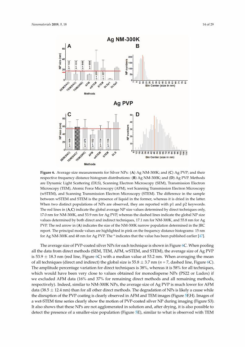
Figure 6. Average size measurements for Silver NPs: (A) Ag NM-300K; and (C) Ag PVP; and their respective frequency distance histogram distributions: (B) Ag NM-300K; and (D) Ag PVP. Methods are Dynamic Light Scattering (DLS), Scanning Electron Microscopy (SEM), Transmission Electron Microscopy (TEM), Atomic Force Microscopy (AFM), wet Scanning Transmission Electron Microscopy (wSTEM), and Scanning Transmission Electron Microscopy (STEM). The difference in the sample between wSTEM and STEM is the presence of liquid in the former, whereas it is dried in the latter. When two distinct populations of NPs are observed, they are reported with p1 and p2 keywords. The red lines in (A,C) indicate the global average NP size values determined by direct techniques only, 17.0 nm for NM-300K, and 53.9 nm for Ag PVP, whereas the dashed lines indicate the global NP size values determined by both direct and indirect techniques, 17.1 nm for NM-300K, and 55.8 nm for Ag PVP. The red arrow in (A) indicates the size of the NM-300K narrow population determined in the JRC report. The principal mode values are highlighted in pink on the frequency distance histograms: 15 nm for Ag NM-300K and 48 nm for Ag PVP. The * indicates that the value has been published earlier [47].

The average size of NM-300K NPs for each technique is shown in Figure 6A. When pooling all the data from direct methods (SEM, TEM, AFM, wSTEM, and STEM), the average size of NM-300K is 17.0 ± 12.3 nm (red line, Figure 6A) with a median value at 14.5 nm. When averaging the mean of all techniques (direct and indirect) the global size is 17.1 ± 3.5 nm (n = 8, dashed line, Figure 6A). Despite the large number of measured NPs (n = 2588), the two performed normality tests failed (GraphPad Prism 5.0). The amplitude percentage variation for direct techniques is 145%, whereas it is 188% with all techniques. These variations, as well as the high standard deviation (SD) value of direct methods, strongly suggest heterogeneity in the NM-300K NPs. The frequency distance histogram of all the direct techniques reveals a multimodal size distribution for NM-300K (Figure 6B). The principal mode is at 15 nm, whereas minor modes are observed at 2, 37, and 54 nm. Indeed, DLS results indicate the presence of two populations (around 2.5 and 22.8 nm), which is confirmed by a careful TEM(SAC) study that identifies two populations around 4.2 and 14.9 nm. Results for the TEM(SAC) column concatenate both populations (Figure 6A). In addition, the surprisingly long tail

Figure 6. Average size measurements for Silver NPs: (A) Ag NM-300K; and (C) Ag PVP; and theirrespective frequency distance histogram distributions: (B) Ag NM-300K; and (D) Ag PVP. Methodsare Dynamic Light Scattering (DLS), Scanning Electron Microscopy (SEM), Transmission ElectronMicroscopy (TEM), Atomic Force Microscopy (AFM), wet Scanning Transmission Electron Microscopy(wSTEM), and Scanning Transmission Electron Microscopy (STEM). The difference in the samplebetween wSTEM and STEM is the presence of liquid in the former, whereas it is dried in the latter.When two distinct populations of NPs are observed, they are reported with p1 and p2 keywords.The red lines in (A,C) indicate the global average NP size values determined by direct techniques only,17.0 nm for NM-300K, and 53.9 nm for Ag PVP, whereas the dashed lines indicate the global NP sizevalues determined by both direct and indirect techniques, 17.1 nm for NM-300K, and 55.8 nm for AgPVP. The red arrow in (A) indicates the size of the NM-300K narrow population determined in the JRCreport. The principal mode values are highlighted in pink on the frequency distance histograms: 15 nmfor Ag NM-300K and 48 nm for Ag PVP. The * indicates that the value has been published earlier [47].

The average size of PVP-coated silver NPs for each technique is shown in Figure 6C. When poolingall the data from direct methods (SEM, TEM, AFM, wSTEM, and STEM), the average size of Ag PVPis 53.9 ± 18.3 nm (red line, Figure 6C) with a median value at 53.2 nm. When averaging the meanof all techniques (direct and indirect) the global size is 55.8 ± 3.7 nm (n = 7, dashed line, Figure 6C).The amplitude percentage variation for direct techniques is 38%, whereas it is 58% for all techniques,which would have been very close to values obtained for monodisperse NPs (PS22 or Ludox) ifwe excluded AFM data (16% and 37% for remaining direct methods and all remaining methods,respectively). Indeed, similar to NM-300K NPs, the average size of Ag PVP is much lower for AFMdata (38.5 ± 12.4 nm) than for all other direct methods. The degradation of NPs is likely a cause whilethe disruption of the PVP coating is clearly observed in AFM and TEM images (Figure 5F,H). Images ofa wet-STEM time series clearly show the motion of PVP-coated silver NP during imaging (Figure S3).It also shows that these NPs are not agglomerated in solution and, after drying, it is also possible todetect the presence of a smaller-size population (Figure 5E), similar to what is observed with TEM


(Figure 5G). The possible degradation of PVP NPs with or without combination with the disruption ofthe PVP coating is likely responsible for the large SD values obtained by all the tested techniques. It isthus not surprising that both normality tests failed for all combined direct technique measurements(n = 960). The frequency distance histogram of all the direct techniques reveals again a broad sizedistribution (Figure 6D), which was not anticipated from individual results since every techniquereported a monomodal distribution (Table S1). The major mode appears at 48 nm while minor modescan be observed at 32, 58, 78, and 88 nm.

3.4. Size Measurements of Titane Dioxide Nanoparticles

Three TiO2 NPs were selected for their interest in nanotoxicology. Suspensions of TiO2 (P25) wereobtained after strong sonication of commercial products; primary particle size of P25 is given around21 nm from the manufacturer and a recent analysis reports a value of 23 ± 10 nm [49]. Due to thehigh temperature synthesis of P25 NPs, they are constituted of two kinds of particles: 75% of anatase,and 25% of rutile. An initial report using TEM indicates that the average size of anatase is 85 nm,whereas that of rutile is 25 nm [66]. TiO2 A12 was determined around 12 nm in size [67]. Food additiveE171 was directly purchased from a manufacturer as a white powder; size of E171 is unknown butusually advertised as above 100 nm in diameter; it is therefore not considered as a nanomaterial inconsumer products. A major difference with previously presented NPs is the strong tendency of allTiO2 NPs to agglomerate, in both liquid and dry conditions (Figure 7), especially for P25 and A12NPs, which are synthesized by gas phase methods (flame spray or laser pyrolysis) usually producingagglomerated materials.

Since the three TiO2 NPs were provided as powders, specific surface areas were determined usingthe BET method: 82 m2/g for A12 (with the density of 3.9; the estimated diameter is 19 nm), 46 m2/gfor P25 (with the density of 3.9; the estimated diameter is 33 nm), and 9.4 m2/g for E171 (with thedensity of 4.0; the estimated diameter is 160 nm). Variations between BET results and global averagevalues from this study range from 21% to 43% (Table S1).

The average size of TiO2 A12 for each technique is shown in Figure 8A. When pooling all the datafrom direct methods (SEM, TEM, AFM, wSTEM, and STEM), the average size of A12 is 10.5 ± 3.8 nm(red line, Figure 8A) with a median value at 9.9 nm. When averaging the mean of all techniques (directand indirect), the global size is 22.5 ± 8.5 nm (n = 8, dashed line, Figure 8A). A total of 100% of A12NPs have a size below 100 nm. Due to the agglomeration of A12 NPs, the DLS-estimated size is verydifferent from other techniques including the indirect SAXS method. It should be remembered that theSAXS instrument used in this study has a cutoff around 30 nm and thus any particles larger than thisthreshold are not seen. The value of 12 ± 2.1 nm from the SAXS technique implies that there mustbe a significant proportion of isolated NPs in the A12 solution. The frequency distance histogram ofall the direct techniques reveals a monomodal size distribution for A12 NPs (Figure 8B); however,despite the large number of measurements (n = 1269), both normality tests failed. The major mode isat 10 nm. The amplitude percentage variation for direct techniques is 119%, whereas it is 293% for alltechniques. Such variations appear in contradiction with the monomodal distribution of determinedNP sizes. If we exclude the value of DLS, the large amplitude variation highlights the precision of thesize measurement itself. Because of the agglomerated state of A12 NPs, it is complicated for AFMimages to measure height values (only NPs at the border of the agglomerate can be analyzed) and it issimilarly challenging to delimit the boundaries of agglomerated NPs using EM methods. In addition,as mentioned earlier, the size of 10 nm is at the technical limit for SEM-based methods. Anotherindication of the difficulty of measurements comes from the comparison of the pooled average sizeof 1269 A12 NPs (10.5 nm) with that of the average of each direct technique mean values (13.6 nm,see Table 1). Except for TEM(GRE), most techniques provided a low number of measurements (near orless than 100) which could also explain the large amplitude variation.



Figure 7. Samples of recorded microscopy images on TiO2 NPs. Images show that, all three NPs, A12, P25, and E171, appear agglomerated in all techniques. Scale bars are indicated on the wSTEM, STEM or SEM images, whereas they appear on top of AFM or TEM images. The AFM image for E171 has been saturated to better visualize smaller NPs present in this sample. The difference between TEM1 and TEM2 images is in the method used for depositing samples: carbon floatation technique for the former or directly onto a carbon-coated grid for the latter (see methods).

Since the three TiO2 NPs were provided as powders, specific surface areas were determined using the BET method: 82 m²/g for A12 (with the density of 3.9; the estimated diameter is 19 nm), 46 m²/g for P25 (with the density of 3.9; the estimated diameter is 33 nm), and 9.4 m²/g for E171 (with the density of 4.0; the estimated diameter is 160 nm). Variations between BET results and global average values from this study range from 21% to 43% (Table S1).

The average size of TiO2 A12 for each technique is shown in Figure 8A. When pooling all the data from direct methods (SEM, TEM, AFM, wSTEM, and STEM), the average size of A12 is 10.5 ± 3.8 nm (red line, Figure 8A) with a median value at 9.9 nm. When averaging the mean of all techniques (direct and indirect), the global size is 22.5 ± 8.5 nm (n = 8, dashed line, Figure 8A). A total of 100% of A12 NPs have a size below 100 nm. Due to the agglomeration of A12 NPs, the DLS-estimated size is very different from other techniques including the indirect SAXS method. It should be remembered that the SAXS instrument used in this study has a cutoff around 30 nm and thus any particles larger than this threshold are not seen. The value of 12 ± 2.1 nm from the SAXS technique implies that there

Figure 7. Samples of recorded microscopy images on TiO2 NPs. Images show that, all three NPs, A12,P25, and E171, appear agglomerated in all techniques. Scale bars are indicated on the wSTEM, STEMor SEM images, whereas they appear on top of AFM or TEM images. The AFM image for E171 hasbeen saturated to better visualize smaller NPs present in this sample. The difference between TEM1and TEM2 images is in the method used for depositing samples: carbon floatation technique for theformer or directly onto a carbon-coated grid for the latter (see methods).



must be a significant proportion of isolated NPs in the A12 solution. The frequency distance histogram of all the direct techniques reveals a monomodal size distribution for A12 NPs (Figure 8B); however, despite the large number of measurements (n = 1269), both normality tests failed. The major mode is at 10 nm. The amplitude percentage variation for direct techniques is 119%, whereas it is 293% for all techniques. Such variations appear in contradiction with the monomodal distribution of determined NP sizes. If we exclude the value of DLS, the large amplitude variation highlights the precision of the size measurement itself. Because of the agglomerated state of A12 NPs, it is complicated for AFM images to measure height values (only NPs at the border of the agglomerate can be analyzed) and it is similarly challenging to delimit the boundaries of agglomerated NPs using EM methods. In addition, as mentioned earlier, the size of 10 nm is at the technical limit for SEM-based methods. Another indication of the difficulty of measurements comes from the comparison of the pooled average size of 1269 A12 NPs (10.5 nm) with that of the average of each direct technique mean values (13.6 nm, see Table 1). Except for TEM(GRE), most techniques provided a low number of measurements (near or less than 100) which could also explain the large amplitude variation.

Figure 8. Average size measurements for TiO2 NPs: (A) A12; (C) P25; and (E) E171; and their respective frequency distance histogram distributions: (B) A12; (D) P25; and (F) E171. Methods are the same as in Figure 6 plus Small-Angle Xray-Scattering (SAXS). The red lines in (A,C,E) indicate the global average NP size values determined by direct techniques only, 10.5 nm for A12, 21.3 nm for P25, and 94.8 nm for E171, whereas the dashed lines indicate the global NP size values determined by both direct and indirect techniques, 22.5 nm for A12, 23.5 nm for P25, and 101.3 nm for E171. The principal mode values are highlighted in pink on the frequency distance histograms: 10 nm for A12, 22 nm for P25, and 85 for E171.

Figure 8. Average size measurements for TiO2 NPs: (A) A12; (C) P25; and (E) E171; and their respectivefrequency distance histogram distributions: (B) A12; (D) P25; and (F) E171. Methods are the same as inFigure 6 plus Small-Angle Xray-Scattering (SAXS). The red lines in (A,C,E) indicate the global averageNP size values determined by direct techniques only, 10.5 nm for A12, 21.3 nm for P25, and 94.8 nmfor E171, whereas the dashed lines indicate the global NP size values determined by both direct andindirect techniques, 22.5 nm for A12, 23.5 nm for P25, and 101.3 nm for E171. The principal modevalues are highlighted in pink on the frequency distance histograms: 10 nm for A12, 22 nm for P25,and 85 for E171.

Table 1. Global average values for NP size determination.

Family NPs Direct Methods All Methods

All Data Pooled(Mean ± SD in nm) n Technique Average

(Mean ± SEM in nm)Technique Average

(Mean ± SEM in nm)

Silver NM-300K 16.8 ± 12.0 2588 18.6 ± 3.8 (n = 6) 17.1 ± 3.5 (n = 8)PVP 53.9 ± 18.3 960 53.3 ± 3.1 (n = 6) 55.8 ± 3.7 (n = 7)

TiO2 A12 10.5 ± 3.8 1269 13.6 ± 2.1 (n = 6) 22.5 ± 8.4 (n = 8)P25 21.3 ± 10.0 2220 21.5 ± 1.5 (n = 6) 23.5 ± 2.3 (n = 7)

E171A 94.8 ± 59.5 1171 95.2 ± 12.9 (n = 6) 101.3 ± 12.5 (n = 7)


The average size of TiO2 P25 for each technique is shown in Figure 8C. When pooling all the datafrom direct methods (SEM, TEM, AFM, wSTEM, and STEM), the average size of P25 is 21.3 ± 10.0 nm(red line, Figure 8C) with a median value at 20.2 nm. When averaging the mean of all techniques(direct and indirect), the global size is 23.5 ± 2.3 nm (n = 7, dashed line, Figure 8C). A total of 100%of P25 NPS have a size below 100 nm. Similar to results obtained with the PVP-coated silver NPs,the homogeneity in global size averages and the large SD values suggest the presence of heterogeneousP25 NPs. The frequency distance histogram of all the direct techniques reveals a multimodal sizedistribution (Figure 8D) with a major mode at 22 nm while minor modes can be observed at 8 or 32nm. Similar to the TiO2 A12 and likely due to agglomeration, DLS average value (35 ± 5 nm, [68])is above every other techniques. The amplitude percentage variation for direct techniques is 40%,whereas it is 77% for all techniques. The broad distribution of P25 sizes near smaller sizes (with aminor mode 12 nm) raised the question why such small size NPs could not be observed in initialTEM measurements (called TEM1). It was decided to perform a second TEM analysis (called TEM2)where the sample was deposited directly on carbon-coated grids, similar to what is performed inAFM. Surprisingly, in TEM2 data, mostly small and isolated P25 NPs (9.8 ± 4.6 nm) were observed onthe carbon grid (Figure 9A). Such results reveal a true operational aspect in NP size determinationwhere small NPs were primarily retained by the mica surface in TEM1 experiment (see methods) andthus absent from the floating carbon layer. The apparent higher binding of small TiO2 NPs on mica(negatively charged surface) is consistent with a lower isoelectric point value for smaller TiO2 NPsthan with larger ones [69].


The average size of TiO2 P25 for each technique is shown in Figure 8C. When pooling all the data from direct methods (SEM, TEM, AFM, wSTEM, and STEM), the average size of P25 is 21.3 ± 10.0 nm (red line, Figure 8C) with a median value at 20.2 nm. When averaging the mean of all techniques (direct and indirect), the global size is 23.5 ± 2.3 nm (n = 7, dashed line, Figure 8C). A total of 100% of P25 NPS have a size below 100 nm. Similar to results obtained with the PVP-coated silver NPs, the homogeneity in global size averages and the large SD values suggest the presence of heterogeneous P25 NPs. The frequency distance histogram of all the direct techniques reveals a multimodal size distribution (Figure 8D) with a major mode at 22 nm while minor modes can be observed at 8 or 32 nm. Similar to the TiO2 A12 and likely due to agglomeration, DLS average value (35 ± 5 nm, [55]) is above every other techniques. The amplitude percentage variation for direct techniques is 40%, whereas it is 77% for all techniques. The broad distribution of P25 sizes near smaller sizes (with a minor mode 12 nm) raised the question why such small size NPs could not be observed in initial TEM measurements (called TEM1). It was decided to perform a second TEM analysis (called TEM2) where the sample was deposited directly on carbon-coated grids, similar to what is performed in AFM. Surprisingly, in TEM2 data, mostly small and isolated P25 NPs (9.8 ± 4.6 nm) were observed on the carbon grid (Figure 9A). Such results reveal a true operational aspect in NP size determination where small NPs were primarily retained by the mica surface in TEM1 experiment (see methods) and thus absent from the floating carbon layer. The apparent higher binding of small TiO2 NPs on mica (negatively charged surface) is consistent with a lower isoelectric point value for smaller TiO2 NPs than with larger ones [56].

Figure 9. Average size measurements for sub-populations of TiO2 NPs: (A) P25; and (B) E171. The larger size populations are colored in yellow, whereas smaller size populations are in orange. Global average of NP sizes within the same technique is colored in pink. The large SD values in AFM data (green columns) prompted checking for the presence of smaller NPs in TEM data by changing the protocol of NPs deposition (TEM1, carbon floatation; and TEM2, direct deposition; see Section 4.3). For both NPs, the TEM2 method identified the presence of smaller NPs than with the TEM1 method, in close agreement with AFM results (which is using a direct deposition method). The global average value of all tested direct techniques is shown in the last column (in red). The two sub-populations observed in wet-STEM were described prior to the change of TEM(GRE) protocol.

Figure 9. Average size measurements for sub-populations of TiO2 NPs: (A) P25; and (B) E171.The larger size populations are colored in yellow, whereas smaller size populations are in orange.Global average of NP sizes within the same technique is colored in pink. The large SD values in AFMdata (green columns) prompted checking for the presence of smaller NPs in TEM data by changingthe protocol of NPs deposition (TEM1, carbon floatation; and TEM2, direct deposition; see Materialsand Methods). For both NPs, the TEM2 method identified the presence of smaller NPs than withthe TEM1 method, in close agreement with AFM results (which is using a direct deposition method).The global average value of all tested direct techniques is shown in the last column (in red). The twosub-populations observed in wet-STEM were described prior to the change of TEM(GRE) protocol.


The average size of TiO2 E171 for each technique is shown in Figure 8E. When pooling all the datafrom direct methods (SEM, TEM, AFM, wSTEM, and STEM), the average size of E171 is 94.8 ± 59.5 nm(red line, Figure 8E) with a median value at 89.7 nm. From direct methods, 57 % of E171 NPs havea size below 100 nm (Table S1). When averaging the mean of all techniques (direct and indirect) theglobal size is 101.3 ± 12.5 nm (n = 7, dashed line, Figure 8E). Similar to all previous TiO2 NPs, addingthe DLS value increases the global E171 size average. This is especially important since averagedsize values are near the cutoff value used for a nanomaterial definition. TiO2 E171 is systematicallyobserved as agglomerates and results for E171 also provide the largest SD values observed in our entirestudy, in agreement with a previous TEM characterization [50], although the global average size islower in our study. The amplitude percentage variation for direct techniques is 86%, whereas it is 98%for all techniques. This large variation in amplitude is mostly due to AFM data that provide an averageE171 size at 38.4 ± 41.8 nm. The frequency distance histogram of all the direct techniques revealsa multimodal size distribution (Figure 8F) with a major mode at 85 nm and a minor mode around10 nm. Similar to P25 NPs, the observed low sizes with AFM prompted us to check another protocolfor TEM imaging. Again, there is a strong operational aspect since the average E171 size determinedwith TEM1 method is 102 ± 39.2 nm, whereas it is 38.2 ± 35.8 nm with TEM2 method (Figure 9B);representative TEM images are shown in Figure 7. The wet-STEM technique also identified a smallsize E171 population around 24.2 ± 8.2 nm and a larger size around 155.1 ± 41.0 nm (Figure 9B).

4. Discussion

The main learning experience from such intercomparison is to present a statistically complete setof data for determining NP sizes accurately with in-house biophysical techniques. Detailed difficultiesof each technique as well as suggested good practice can be found in the Supplementary Materials.

Let us briefly summarize the main characteristics of major techniques used in this study byclassifying them into two categories: direct and indirect techniques.

Direct methods produce images onto which size measurements can be directly performed andwhere the uncertainties are determined from the size distribution. Electron Microscopies (EM) provide2D images with a greater contrast for NPs with high atomic number elements and a resolution below1 nm. Size measurements are usually performed manually (shape recognition software can also beused if the contrast is satisfactory) by identifying and labeling NPs on an image and by estimating thepixel length of their diameter. It is difficult to characterize aggregates with EM (lack of 2D contrast)and it is not sensitive to the organic capping often present on commercial NPs. Due to its higherresolution, TEM is often preferred to SEM for characterization of NPs with a size below about 20 nm.Wet-Scanning Transmission Electron Microscopy (wet-STEM) consists in implementing a dedicatedwet-STEM stage in any Environmental SEM (ESEM). This approach allows the observation of NPsin liquid state at first, and when the liquid layer evaporates, dry NPs can be visualized. Althoughthe thinning of the liquid film can be tricky during introduction of the sample in the ESEM chamber,it takes no more than 30 min from the grid preparation to sample observation (see Methods for moredetails). This technique allows the recording of images with a 3 nm lateral resolution at 30 kV [70],which makes possible the observation for most of the nanoparticles having a diameter higher than 6 nm.AFM, the other microscopy-based technique, produces images of a sample deposited on a flat substrate(usually mica or graphite). Images are obtained by rastering a nanosize tip over the sample whichmakes AFM a “touching” microscopy technique. AFM images encode at each pixel the height value ofthe probed sample area. Accordingly, AFM is the only direct technique that can provide a real directthree-dimensional size analysis of a single NP. AFM height values are characterized with a resolutionbelow 1 nm; however, due to the tip convolution effect which distorts AFM images, AFM lateral sizesdepends on the size and shape of the AFM tip, which always produced an overestimation of x-axisand y-axis dimensions. Depending on the applied force on the AFM tip, AFM technique can detectorganic capping of NPs. Size measurements can be performed automatically if NPs are sufficiently


isolated by taking the tallest height value of a NP of interest from the image; however, in the case ofNP agglomeration, manual cross-section profile can be used to extract size values.

Indirect techniques require a physical model to extract NP size from the raw experimentalsignal. For light scattering techniques (e.g., DLS), the Raleigh scattering dictates that the light intensityscattered by a NP is proportional to its diameter raised to the sixth power; thus, large diameterNPs will dominate the intensity signal and even a low population of large particles can makedifficult the detection and analysis of a population of small size. A polydispersity index >0.1 limithas been suggested, above which DLS can no longer be interpreted [39]. DLS uncertainty is based onmeasurement repeatability. Modern instruments provide the analysis directly within the controllingsoftware by giving an average hydrodynamic radius for each detected population. SAXS technique iswell developed for determining NP sizes of simple geometric shape, but the requirement for measuringat very low angle, for large particles, usually requires specific instruments not often found in commondepartments. Moreover, the objects should present a sufficiently high electronic contrast with thesurrounding continuous phase. Measurement of SAXS uncertainty is often fixed at 10%, a value basedon previous experiences in the NIST laboratory.

The goal of NP size characterization is to provide a statistical estimate of the average size of theirprimary elements. This is, however, not a trivial quest. Intercomparison experiments assume that all thetested techniques determine a similar measurand. According to the metrology definition, a measurandis the parameter to be measured. In this work, the goal was to measure the diameter of NPs (or theirradius). However, all tested techniques in this work did not determine the same measurand: fordirect methods (microscopies), it is a geometrical diameter (or radius), whereas, for indirect methods(light scattering or SAXS), it is rather a hydrodynamic radius. For mono-dispersed and sphericalisolated NPs in solution, both geometric and hydrodynamic radii should provide very similar values.This is in agreement with our results when considering the non-agglomerated and monodispersedsamples (nanosphere and Ludox series) where no significant deviations are observed between directand indirect techniques (one-way ANOVA test for all NPs measured in this work).

The classical representation of a sample from a population is to provide a mean value and astandard deviation (SD) around the mean. Without considering the shape of the true underlyingdistribution, the mean and SD are sufficient in most cases where NPs are mainly spherical, isolated,and monodispersed. In this work, this was the case only for model NPs (PS22 beads or solubilizedsilicate NPs Ludox) where both direct and indirect techniques provide a good estimate of the averageNP size. Unfortunately, results in this work were different from the “realistic” NPs (silver and titaniumoxide), where a strong heterogeneity in size or in agglomeration was observed (see frequency distancehistograms in Figures 6 and 8). It should be emphasized that size heterogeneity may be native(present during the fabrication of NPs) or due to degradations, as observed for silver NPs (Figure 5).Alternatively, results could also be expressed as a range which has often been the case in recentreports for P25 NPs (30–40 nm [71] or 500–2400 nm (aggregates) [72]) or for E171 NPs (31–200 nm [73],30–600 nm [74], of 50–250 nm [75]). Sometimes, a range is even not provided but instead the ratio oftrue NPs (<100 nm) [76]. Nevertheless, range values are difficult to handle when attempting to comparedistribution in sizes. The other frequently used size measurement is the median. It has a superiorityover the classical mean in that it is less sensitive to extreme values when the number of measurementsis limited. Most computed medians on NPs match closely the values of their corresponding mean,except for E171. Indeed, TiO2 E171 is a special case since, with all techniques, the average size is101.3 nm, whereas it is only 94.8 nm with direct techniques. In addition, it was found that 53% ofE171 NPs have a size below 100 nm. Thus, according to our results, this particular lot of E171 is at thethreshold of the NP definition and a deeper investigation would be required to make a final judgmentconcerning the classification of this lot of E171 as NPs.

Another challenge in providing a proper size description of NPs is to evaluate the need to describesub-populations. All difficulties could be summarized with a single term: proportion estimation.In other words: Is it possible to quantify the proportion of mixed NPs simply by looking at a couple of


images for direct techniques? This difficulty for direct techniques is alleviated for indirect ones sinceit is often possible to fit data (for instance, DLS and SAXS) using different models that may includevarious sub-populations. However, adding contributions to fit experimental data should be consideredcarefully: the increase of fitting parameters always results in a better agreement between calculatedand experimental profiles, but can also result in misleading interpretations.

For a regulatory purpose, size characterization of NPs simply needs to answer the questionwhether at least 50% in number of primary particles have at least one external dimension size below100 nm. Unfortunately, there is no existing method to answer such a complex question [77]. For instance,indirect methods are incapable of distinguishing primary particles from agglomerated NPs and directmethods cannot guarantee a sufficiently large sampling of NPs to ascertain the 50% threshold value.This is particularly critical for heterogeneous NPs (such as TiO2 E171) where the average size of primaryparticles is around the 100 nm threshold in diameter. For a toxicological purpose, size characterizationof NPs needs to describe all the possible sub-populations of NPs to make sure that identified functionalresults are really correlated with true NPs. Indeed, as described in the Introduction, sometimes acouple of tens of nm in a NP size could make a difference in toxicological tests. Whatever the purpose,it seems that a frequency distance histogram is the best answer when NPs are heterogeneous (either inintrinsic primary particle sizes or in agglomerated shape), which were all the “realistic” NPs tested inthis work (silver and TiO2). It is likely not the easiest way but the combination of several direct methodscoupled with different experimental setups are most likely to avoid any mis-characterization of NPssizes. From a histogram, it is possible to extract an average value, a modal value, and the amplitudeof values. From our results, Gaussian curve fitting did not provide a better characterization since nofrequency distance distribution followed normality. Sub-populations were mostly visually identifiedby locating gaps in the histograms; there is likely room for improvement. For strictly monodisperseNPs, indirect methods are the best choice due to their simplicity and a single confirmation with asingle direct method will ascertain that the average value between indirect and direct methods match.

Operational aspects are unexpected consequences of particular choices of experimental setupsand they have been observed numerous times [78–80] since their first description [81]. The best-knownoperational aspect in NP size determination is the physical state of NPs. Due to their chemical naturesor due to the environment (presence of salts and proteins from buffers or culture media), NPs have beenknown to agglomerate and aggregate [8,13,16,26,29,35,39,43,45,65]. Besides, due to its high energeticadhesive forces, which contribute to adsorbing proteins or small molecules, the surface of a NP israrely “bare” [4], especially in biological media. Therefore, their size increases/decreases upon theagglomeration/disruption status of a given NP. Several studies focus on sample preparation andsample homogenization, where many efforts are targeted to the dispersion problem of NPs [29,33],including in nanotoxicology studies [68], and encouraging results have been found for specificNPs [43–45,82]. Although methods exist to model multimodal distribution of NPs using light scatteringand SAXS techniques [83], a recent study reveals that the observation of multimodal dispersion ofisobutylcyanoacrylate-based NPs only succeeded by AFM, nanoparticle tracking analysis, and tunableresistive pulse sensing techniques [33], whereas no light scattering batch methods could reproduce theparticle size distribution.

A second level of the impact of operational aspects lies in the experimental protocol. It has beenshown that two of the major biophysical techniques used for NP size determination (TEM and DLS)were the most prone to artifacts [36]. Such a claim is not used to disqualify these techniques regardingNP size determination, but rather to encourage researchers to pay closer attention to the protocol used.Drying samples is a classical criticism of microscopy techniques (EM and AFM), although a recentanalysis reports that dry conditions in AFM is not the major hurdle in determining the correct heightof a virus [80]. In fact, the nature of the substrate used to deposit a virus has been found to be the mostsensitive parameter toward proper height measurement with AFM [80]. Such phenomenon has againbeen proven in this work, where NPs sizes obtained from TEM results were very different accordingto the method used to deposit the sample. In the first case (TEM1), a competition between mica and


carbon layer was possible, whereas, in the second case (TEM2), only the contact with a carbon layerwas allowed. When the TiO2 NP does not have a significant adsorption preference between micaand carbon layer, such as the TiO2 A12 NPs, determined sizes remain very similar in both methods(Table S1). However, for TiO2 P25 and E171, a difference between this adsorption led to characterize atotally different spectrum of NP sizes (Figure 9). Interestingly, the wet-STEM technique reveals thepresence of both small and large E171 NPs which implies that both sizes are simultaneously presentin the sample (Figure 9). The distinction between wSTEMp1 and wSTEMp2 was made at the verybeginning of the analysis without knowing the unexpected behavior of E171 with carbon layers andmica. A similar observation was observed for TEM(SAC) on NM-300K NPs, where depending onthe EM grids, a majority of small Ag NM-300K NPs could be observed when the Lacey carbon grids(with holes) were used (Figure S4).

The third level of the impact of operational aspect depends on the perspicacity of the humanoperator as defined by Eisenhart. It mostly pertains to the identification of multimodal NP sizedistribution. The case of the Ag NM-300K NPs is the most interesting. This NM-300K NP is part ofrepresentative manufactured nanomaterials from the European Commission Joint Research Center(JRC). A report provides a description of this nanomaterial as “silver particles of about 15 nm sizewith a narrow size distribution of 99 % of the particle number concentration exhibiting a diameterof below 20 nm” [51]. The report mentions the presence of smaller NPs (~5 nm) only observed withTEM, whereas larger NPs (~50–60 nm) have been observed with both NTA and DLS techniques. In thiswork, both minor species of NPs were observed: DLS and TEM for the small sizes, and wSTEM,AFM, and TEM for large sizes. It should be added that the small population found in TEM(SAC) hasbeen pursued after the JRC report mentioned the presence of such small NPs. As seen in Figure 5A,wSTEM (and also STEM) data clearly reveal the presence of a majority of large size NM-300K NPs andconsequently it was initially reported as a specific sub-population of this NP. Large NM-300K NPswere also observed with AFM and TEM(GRE) (see Figure 5B,C), however, their proportion relative tothe “normal” size NM-300K is small (less than 1% of NM-300K was larger than 25 nm according toTEM data). Consequently, by pooling all the TEM(GRE) measures together, the impact of large NPsbecame minor on the average NP size. In AFM, such large NM-300K NPs were not taken into accountsince it was not possible to accurately determine their height because these large NPs sat on top ofother NPs. Compared to our NM-300K direct technique-based average size of 16.8 ± 12.0 nm (Table 1),a recent study using traditional and tabletop TEMs provides similar values albeit with a narrowerrange in the NP size determination of NM-300K, 17.2 ± 5.5 nm and 19.1 ± 3.3 nm, respectively [84].Quantification of sub-population proportions is a major challenge for metrological characterizationof nanomaterials. The main difficulty is first to sample a very large number of NPs and second tomake sure that the protocol used for size determination does not introduce a systematic bias as foundabove in EM or AFM. There is possibly another “human operator” impact in NP size determinationand it is best illustrated with the TiO2 A12 NPs. All tested direct techniques (Figure 8A) but two,TEM(SAC) and AFM, observed a normality in the distribution of NP size values. This property isnot correlated with the population size in each technique (normality was observed in the range of20–843 NPs). Surprisingly, when pooling all the direct techniques data, normality tests failed on a totalof 1269 NPs. It is possible that a miscalibration of some instruments is the cause of such phenomenon,albeit unlikely since there is no consistent bias toward low or high values among all the tested directtechniques. Another possibility is a sense of “dejà-vu” when an operator unconsciously manuallyselects mostly particles that resemble one another. If all NPs of an image cannot be selected (due tosome agglomeration or border locations), the selection of NPs should not be restrained to those having“good similarities” to others.

Finally, the fourth level of the impact of the operational aspects is time. As seen with silver NPs,degradation of NPs is interactively measured (Figure 5D), implying that their stability upon time is amajor concern. Beside the time, there could be an instrument bias causing the degradation of silver NPs.Indeed, AFM technique uses a red laser to detect changes in the contact between the sample surface


and the AFM tip as well as a white light for the camera which may increase the rate of degradation ofsilver NPs. Thus, for light-sensitive NPs such as silver, AFM technique should minimize lighting oruse a “dark mode” with piezoelectric tuning fork imaging [85].

What are the recommendations for proper NP size determination? First, choosing differentbiophysical techniques should reduce artifacts present in each known technique (direct or indirect).The presence of at least one direct technique is strongly recommended. Besides, providing an averageacross several techniques is likely more robust than any single technique. When a single techniqueprovides an unusually different size estimation (e.g., DLS on A12 NPs in this work), it is then importantto look carefully in every technique to highlight potential operational biases and, if not, the outlierresult should be discarded in the final average. It is equally important to know the technical limitationsof each method and it is always safer to contact specialist operators. Second, it is critical to makeenough measurements regarding direct microscopy techniques. For monodispersed NPs, a rangebetween 100 and 300 is mostly adequate. Measuring more than 300 sizes did not change the shape of amonomodal distribution. However, for heterogeneous NPs, our study cannot provide an upper limitsince results from apparent monomodal distributions could not reach statistical normality with upto 2000 measurements. Although the normality distribution is not a goal in NPs size determination,we suggest that a minimum of 300 values per identified mode be the target value in number ofmeasures. Third, do not make an educated guess about the expected size of NPs as we have seen inour work that an inter-technique amplitude variation of 300% is possible. There are multiple reasonsfor a similar NP to display large variations in its size: choice of techniques, impact of operationalaspects, operator variability, degradation, etc. Fourth, it is equally critical to modify the experimentalprotocols to detect minor sub-populations. Modifications include change of concentration, change ofdeposition time, change of deposition method, change of substrate for imaging techniques, change inmeasurement methods, change in measurement software, and change in operators. This is importantbecause changing experimental conditions will limit the influence of operational aspects. For example,changing the imaging mode or the image substrate in AFM (or grids in EM) should clearly be countedas two different biophysical characterizations. Fifth, it is important to harmonize the number ofNPs counted per physical record (in microscopy, one record is one image). For instance, if a largeNP (agglomerate) breaks into smaller pieces, it could be counted as hundreds of small particles.When adding several hundred “artifacts” values into a statistic, it will necessarily bias the final sizeevaluation; instead, if an average image contains 50 particles, then it is a safe practice to only measurearound 50 particles per image. It is also strongly recommended to include minority sizes (small orlarge in size) to detect minor sub-populations of a sample that may present a strong bias from image toimage. Sixth, keep appropriate records of measurement periods as NPs are subject to deteriorationupon time (as it was found for the silver NPs in AFM). If NP size determination is performed at thereception of NPs, it would be necessary to repeat the size measurements if biological experimentsusing these NPs are not concomitant with their reception.

5. Conclusions

Nanotoxicology research aims at determining the potential harm of a given nanoparticle,especially regarding their size. Attributing a toxicological effect to the proper range of NP sizesis a major challenge and it is likely that some controversies in the effect of NPs sizes on cells or tissuescould be due to poor characterization of the NP solutions used in toxicological tests. It is therefore ofmajor importance to provide careful statistical evaluation of the performance of biophysical techniquesused to determine NPs sizes. In this study, we aimed at using “standard” laboratory instruments tothe best of their capacity without any preparation constraints and therefore following local laboratoryprotocols. Final NPs size averages were obtained by averaging data from all the available technique,which, in most cases, provided a consolidated result of a given primary NP size.

The six different biophysical techniques used in this study (DLS, TEM, SEM, SAXS, AFM,and wSTEM) provide similar results when characterizing the size of monodispersed nanoparticles


(average amplitude variations of 25%). Interestingly, on these monodispersed NPs, the variation insize within each technique (using different experimental setup) is about the same as the variationamong all six techniques. A summary of “realistic” NPs sizes determined in this study is found inTable 1. As expected, the average inter-technique deviations increased when size characterizationinvolved agglomerated NPs or multimodal distributions; a maximum amplitude variation of 300%was found between DLS and EM. Most importantly, variations in size determination was not onlyan intrinsic limitation of each individual technique but included: (1) the presence of mixed size NPsand the lack of recognition of some minor populations; (2) the degradation of NPs; (3) the operationalaspects (experimental details that bias unintentionally measurements by capturing/excluding someNPs populations); and (4) the NP agglomeration that challenges the operator for individual NP sizemeasurements (identification of the “correct” edge of NPs for instance). We would like to emphasizethat NP size characterization is a complex problem that requires a full attention (especially to details)and cannot be assigned to inexperienced operators/analysts in NP size characterization. We stronglyadvise combining several biophysical techniques, both direct and indirect, and to perform variationsin measurement setups (sample dilutions, various grids for EM, various substrates or imaging modesfor AFM, different dispersion protocols for DLS, etc.) and to take the global average of all thesetechniques as the average size of a NP. For complex NP size distribution (multimodal), a histogram ofthe distribution is necessary or a report of the different detected modes.

Regarding the applicability of tested techniques on NPs size determination, the two tested indirecttechniques, SAXS and DLS, were totally reliable on monodisperse NPs in solutions, whereas onlythe SAXS technique was reliable for “realistic” heterogeneous NPs. Even with modern analysis inDLS, this technique is of little help to identify primary particles when NPs are agglomerated, but,due to its ease of use, DLS could be a first choice technique for an initial characterization of unknownNP samples, on the condition that the presence of agglomerated NPs be detected by the instrumentanalysis software. Single NP imaging remains a central method for all kinds of NPs where TEM willbe preferred over SEM for smaller NPs, AFM will be preferred for non-spherical NPs or imaging inliquid environment as does the wet-STEM technique. All the direct techniques suffer from a majorinconvenience, i.e., the necessity to deposit NPs on a flat surface, which has been shown to cause majoroperational limitations. The main challenges with EM-based techniques are the precise identificationof the edge of NPs to provide accurate size values and the lack of characterization in third dimensionscould be a major hurdle for non-spherical NPs. Wet-STEM is a relatively new EM-based techniquefor NPs; it allows the imaging of NPs while in liquid solution and may become a critical advantagewhen NP agglomeration is provoked through drying. AFM technique is another direct technique, but,to the contrary of EM-based techniques, AFM images contain physical height measurements and canprovide size values in three-dimension (with an x–y plane limitation due to tip convolution). Thus,AFM is likely the method of choice when the shape of NPs is far away from spherical. Evaluating theshape of NPs remains the next important challenge in nanotoxicology.

Supplementary Materials: The following are available online at http://www.mdpi.com/2079-4991/9/1/18/s1,Content of Supplementary Data: Text: Difficulties and recommendations for evaluating NPs size, Table S1:Global results of silver and TiO2 nanoparticle size measurements provided by all the participants, Figure S1:Wet-STEM time series for silver NM-300K nanoparticles, Figure S2: High magnification of NM-300K NPs observedwith wSTEM. Figure S3: Wet-STEM time series for PVP-coated silver nanoparticles, Figure S4: TEM images ofsilver NM-300K NPs on two different grid supports, Figure S5: Two different methods to measure NPs sizes(Ludox TM-50).

Author Contributions: Conceptualization, J.-L.P., J.C., R.P. and N.H.-B.; Methodology, J.-M.T., C.G., L.C., C.M.,J.C., R.P., M.O., J.R., A.G., and A.H.; Software, S.-w.W.C.; Formal Analysis, S.-w.W.C., J.C., R.P., N.H.-B. and J.-L.P.;Writing—Original Draft Preparation, J.L.P.; Writing—Review and Editing, J.-M.T., C.G., J.C., R.P., N.H.-B. andJ.-L.P.; and Supervision, J.-L.P.

Funding: This research was funded by the grant “AFM-nanotox” from the CEA “programme transversalToxicologie et Nanosciences”. We thank Guy Schoehn and the platforms of the Grenoble Instruct-ERICCenter (ISBG: UMS 3518 CNRS-CEA-UGA-EMBL) with support from FRISBI (ANR-10 INSB-05-02) and GRAL(ANR-10-LABX-49-01) within the Grenoble Partnership for Structural Biology (PSB). The electron microscope

http://www.mdpi.com/2079-4991/9/1/18/s1


facility is supported by the Auvergne-Rhône-Alpes Region, the Fondation Recherche Medicale (FRM), the fondsFEDER, the Centre National de la Recherche Scientifique (CNRS), the CEA, the University of Grenoble, EMBL,and the GIS-Infrastrutures en Biologie Sante et Agronomie (IBISA).

Acknowledgments: The initial part of this work was inspired by discussions at the European COST ActionTD1002: AFM4NanoMed&Bio within the working group 4 (http://afm4nanomedbio.eu/working-group-4.aspx):Vesna Svetlicic, Tea Mišic and Galja Pletikapic (IRB Zagreb), Alessandro Podestà (Univ. Milano), Jean-NicolasAudinot (Luxembourg Inst. Sci. Technol.). We thank Marie Carrière (CEA/INAC Grenoble) for her adviceconcerning nanoparticles. We acknowledge the TEM-team CEA/DRF platform for the use of TEM Philips.

Conflicts of Interest: The authors declare no conflict of interest.

References

1. Rauscher, H.; Roebben, G.; Amenta, V.; Sanfeliu, A.B.; Calzolai, L.; Emons, H.; Gaillard, C.; Gibson, N.;Linsinger, T.; Mech, A.; et al. Towards a Review of the Ec Recommendation for a Definition of the Term“Nanomaterial”. Part 1: Compilation of Information Concerning the Experience with the Definition. In JRCReference Reports; Rauscher, H., Roebben, G., Eds.; Joint Research Centre: Luxembourg, 2014; p. 288, ISBNJRC89369.

2. European Commission. Commission Recommendation of 18 October 2011 on the Definition of Nanomaterial.Off. J. Eur. Union 2011, 275, 38–40.

3. Linsinger, T.; Roebben, G.; Gilliland, D.; Calzolai, L.; Rossi, F.; Gibson, N.; Klein, C. Requirements onMeasurements for the Implementation of the European Commission Definition of the Term “Nanomaterial”.In JRC Reference Reports; Publications Office of the European Union: Luxembourg, 2012; ISBN JRC73260.

4. Borm, P.J.; Robbins, D.; Haubold, S.; Kuhlbusch, T.; Fissan, H.; Donaldson, K.; Schins, R.; Stone, V.;Kreyling, W.; Lademann, J.; et al. The Potential Risks of Nanomaterials: A Review Carried out for Ecetoc.Part. Fibre Toxicol. 2006, 3, 11. [CrossRef] [PubMed]

5. Bhatia, S. Nanoparticles Types, Classification, Characterization, Fabrication Methods and Drug DeliveryApplications. In Natural Polymer Drug Delivery Systems; Springer: Cham, Switzerland, 2016; pp. 33–93.

6. The Royal Society & The Royal Academy of Engineering. Nanoscience and Nanotechnologies: Opportunities andUncertainties; The Royal Society: London, UK, 2004; p. 116, ISBN 0854036040.

7. Scientific Committee on Consumer Products. Safety of Nanomaterials in Cosmetic Products; EU Commission:Luxembourg, 2007; p. 63.

8. Klaine, S.J.; Alvarez, P.J.; Batley, G.E.; Fernandes, T.F.; Handy, R.D.; Lyon, D.Y.; Mahendra, S.;McLaughlin, M.J.; Lead, J.R. Nanomaterials in the Environment: Behavior, Fate, Bioavailability, and Effects.Environ. Toxicol. Chem. 2008, 27, 1825–1851. [CrossRef] [PubMed]

9. Oberdorster, G.; Ferin, J.; Lehnert, B.E. Correlation between Particle Size, in Vivo Particle Persistence,and Lung Injury. Environ. Health Perspect. 1994, 102 (Suppl. 5), 173–179. [PubMed]

10. Donaldson, K.; Stone, V.; Tran, C.L.; Kreyling, W.; Borm, P.J. Nanotoxicology. Occup. Environ. Med. 2004, 61,727–728. [CrossRef] [PubMed]

11. Duffin, R.; Tran, L.; Brown, D.; Stone, V.; Donaldson, K. Proinflammogenic Effects of Low-Toxicity and MetalNanoparticles in Vivo and in Vitro: Highlighting the Role of Particle Surface Area and Surface Reactivity.Inhal. Toxicol. 2007, 19, 849–856. [CrossRef] [PubMed]

12. Powers, K.W.; Brown, S.C.; Krishna, V.B.; Wasdo, S.C.; Moudgil, B.M.; Roberts, S.M. Research Strategiesfor Safety Evaluation of Nanomaterials. Part Vi. Characterization of Nanoscale Particles for ToxicologicalEvaluation. Toxicol. Sci. 2006, 90, 296–303. [CrossRef] [PubMed]

13. Nel, A.; Xia, T.; Madler, L.; Li, N. Toxic Potential of Materials at the Nanolevel. Science 2006, 311, 622–627.[CrossRef]

14. Kobayashi, N.; Izumi, H.; Morimoto, Y. Review of Toxicity Studies of Carbon Nanotubes. J. Occup. Health2017, 59, 394–407. [CrossRef]

15. Chalupa, D.C.; Morrow, P.E.; Oberdorster, G.; Utell, M.J.; Frampton, M.W. Ultrafine Particle Deposition inSubjects with Asthma. Environ. Health Perspect. 2004, 112, 879–882. [CrossRef]

16. Zook, J.M.; Maccuspie, R.I.; Locascio, L.E.; Halter, M.D.; Elliott, J.T. Stable Nanoparticle Aggregates/Agglomerates of Different Sizes and the Effect of Their Size on Hemolytic Cytotoxicity. Nanotoxicology 2011,5, 517–530. [CrossRef] [PubMed]

http://afm4nanomedbio.eu/working-group-4.aspx

http://dx.doi.org/10.1186/1743-8977-3-11

http://www.ncbi.nlm.nih.gov/pubmed/16907977

http://dx.doi.org/10.1897/08-090.1



http://dx.doi.org/10.1136/oem.2004.013243


http://dx.doi.org/10.1080/08958370701479323


http://dx.doi.org/10.1093/toxsci/kfj099


http://dx.doi.org/10.1126/science.1114397

http://dx.doi.org/10.1539/joh.17-0089-RA

http://dx.doi.org/10.1289/ehp.6851

http://dx.doi.org/10.3109/17435390.2010.536615



17. Hossain, S.T.; Mukherjee, S.K. Cdo Nanoparticle Toxicity on Growth, Morphology, and Cell Division inEscherichia Coli. Langmuir 2012, 28, 16614–16622. [CrossRef] [PubMed]

18. George, I.; Naudin, G.; Boland, S.; Mornet, S.; Contremoulins, V.; Beugnon, K.; Martinon, L.; Lambert, O.;Baeza-Squiban, A. Metallic Oxide Nanoparticle Translocation across the Human Bronchial Epithelial Barrier.Nanoscale 2015, 7, 4529–4544. [CrossRef] [PubMed]

19. Yang, X.; Liu, J.; He, H.; Zhou, L.; Gong, C.; Wang, X.; Yang, L.; Yuan, J.; Huang, H.; He, L.; et al. SiO2

Nanoparticles Induce Cytotoxicity and Protein Expression Alteration in Hacat Cells. Part. Fibre Toxicol. 2010,7, 1. [CrossRef] [PubMed]

20. Tarantini, A.; Lanceleur, R.; Mourot, A.; Lavault, M.T.; Casterou, G.; Jarry, G.; Hogeveen, K.; Fessard, V.Toxicity, Genotoxicity and Proinflammatory Effects of Amorphous Nanosilica in the Human Intestinal Caco-2Cell Line. Toxicol. Vitro 2015, 29, 398–407. [CrossRef] [PubMed]

21. Chen, M.; von Mikecz, A. Formation of Nucleoplasmic Protein Aggregates Impairs Nuclear Function inResponse to SiO2 Nanoparticles. Exp. Cell Res. 2005, 305, 51–62. [CrossRef] [PubMed]

22. Vogt, A.; Combadiere, B.; Hadam, S.; Stieler, K.M.; Lademann, J.; Schaefer, H.; Autran, B.; Sterry, W.;Blume-Peytavi, U. 40 Nm, but Not 750 or 1,500 Nm, Nanoparticles Enter Epidermal Cd1a+ Cells afterTranscutaneous Application on Human Skin. J. Investig. Dermatol. 2006, 126, 1316–1322. [CrossRef]

23. Jallouli, Y.; Paillard, A.; Chang, J.; Sevin, E.; Betbeder, D. Influence of Surface Charge and Inner Compositionof Porous Nanoparticles to Cross Blood-Brain Barrier in Vitro. Int. J. Pharm. 2007, 344, 103–109. [CrossRef]

24. Yin, H.; Too, H.P.; Chow, G.M. The Effects of Particle Size and Surface Coating on the Cytotoxicity of NickelFerrite. Biomaterials 2005, 26, 5818–5826. [CrossRef]

25. Warheit, D.B.; Webb, T.R.; Sayes, C.M.; Colvin, V.L.; Reed, K.L. Pulmonary Instillation Studies with NanoscaleTiO2 Rods and Dots in Rats: Toxicity Is Not Dependent Upon Particle Size and Surface Area. Toxicol. Sci.2006, 91, 227–236. [CrossRef]

26. Sohaebuddin, S.K.; Thevenot, P.T.; Baker, D.; Eaton, J.W.; Tang, L. Nanomaterial Cytotoxicity Is Composition,Size, and Cell Type Dependent. Part. Fibre Toxicol. 2010, 7, 22. [CrossRef] [PubMed]

27. Strobel, C.; Forster, M.; Hilger, I. Biocompatibility of Cerium Dioxide and Silicon Dioxide Nanoparticles withEndothelial Cells. Beilstein J. Nanotechnol. 2014, 5, 1795–1807. [CrossRef] [PubMed]

28. Dwivedi, M.V.; Harishchandra, R.K.; Koshkina, O.; Maskos, M.; Galla, H.J. Size Influences the Effect ofHydrophobic Nanoparticles on Lung Surfactant Model Systems. Biophys. J. 2014, 106, 289–298. [CrossRef][PubMed]

29. Brydson, R.; Brown, A.; Hodges, C.; Abellan, P.; Hondow, N. Microscopy of Nanoparticulate Dispersions.J. Microsc. 2015, 260, 238–247. [CrossRef] [PubMed]

30. Brunauer, S.; Emmett, P.H.; Teller, E. Adsorption of Gases in Multimolecular Layers. J. Am. Chem. Soc. 1938,60, 309–319. [CrossRef]

31. Shang, J.; Gao, X. Nanoparticle Counting: Towards Accurate Determination of the Molar Concentration.Chem. Soc. Rev. 2014, 43, 7267–7278. [CrossRef] [PubMed]

32. MacCuspie, R.I.; Rogers, K.; Patra, M.; Suo, Z.; Allen, A.J.; Martin, M.N.; Hackley, V.A. Challenges forPhysical Characterization of Silver Nanoparticles under Pristine and Environmentally Relevant Conditions.J. Environ. Monit. 2011, 13, 1212–1226. [CrossRef] [PubMed]

33. Varenne, F.; Makky, A.; Gaucher-Delmas, M.; Violleau, F.; Vauthier, C. Multimodal Dispersion of Nanoparticles:A Comprehensive Evaluation of Size Distribution with 9 Size Measurement Methods. Pharm. Res. 2016, 33,1220–1234. [CrossRef]

34. Wilkinson, K.J.; Balnois, E.; Leppard, G.G.; Buffle, J. Characteristic Features of the Major Components ofFreshwater Colloidal Organic Matter Revealed by Transmission Electron and Atomic Force Microscopy.Colloids Surf. A 1999, 155, 287–310. [CrossRef]

35. Murdock, R.C.; Braydich-Stolle, L.; Schrand, A.M.; Schlager, J.J.; Hussain, S.M. Characterization ofNanomaterial Dispersion in Solution Prior to in Vitro Exposure Using Dynamic Light Scattering Technique.Toxicol. Sci. 2008, 101, 239–253. [CrossRef]

36. Domingos, R.F.; Baalousha, M.A.; Ju-Nam, Y.; Reid, M.M.; Tufenkji, N.; Lead, J.R.; Leppard, G.G.;Wilkinson, K.J. Characterizing Manufactured Nanoparticles in the Environment: Multimethod Determinationof Particle Sizes. Environ. Sci. Technol. 2009, 43, 7277–7284. [CrossRef] [PubMed]

37. Aimable, A.; Bowen, P. Nanopowder Metrology and Nanoparticle Size Measurement—Towards theDevelopment and Testing of Protocols. Process. Appl. Ceram. 2010, 4, 157–166. [CrossRef]

http://dx.doi.org/10.1021/la302872y


http://dx.doi.org/10.1039/C4NR07079H


http://dx.doi.org/10.1186/1743-8977-7-1


http://dx.doi.org/10.1016/j.tiv.2014.10.023


http://dx.doi.org/10.1016/j.yexcr.2004.12.021


http://dx.doi.org/10.1038/sj.jid.5700226

http://dx.doi.org/10.1016/j.ijpharm.2007.06.023

http://dx.doi.org/10.1016/j.biomaterials.2005.02.036

http://dx.doi.org/10.1093/toxsci/kfj140

http://dx.doi.org/10.1186/1743-8977-7-22


http://dx.doi.org/10.3762/bjnano.5.190


http://dx.doi.org/10.1016/j.bpj.2013.10.036


http://dx.doi.org/10.1111/jmi.12290


http://dx.doi.org/10.1021/ja01269a023

http://dx.doi.org/10.1039/C4CS00128A


http://dx.doi.org/10.1039/c1em10024f


http://dx.doi.org/10.1007/s11095-016-1867-7

http://dx.doi.org/10.1016/S0927-7757(98)00874-7

http://dx.doi.org/10.1093/toxsci/kfm240

http://dx.doi.org/10.1021/es900249m


http://dx.doi.org/10.2298/PAC1003157A


38. Roebben, G.; Ramirez-Garcia, S.; Hackley, V.A.; Roesslein, M.; Klaessig, F.; Kestens, V.; Lynch, I.; Garner, C.M.;Rawle, A.; Elder, A.; et al. Interlaboratory Comparison of Size and Surface Charge Measurements onNanoparticles Prior to Biological Impact Assessment. J. Nanopart. Res. 2011, 13, 2675–2687. [CrossRef]

39. Baalousha, M.; Lead, J.R. Rationalizing Nanomaterial Sizes Measured by Atomic Force Microscopy, FlowField-Flow Fractionation, and Dynamic Light Scattering: Sample Preparation, Polydispersity, and ParticleStructure. Environ. Sci. Technol. 2012, 46, 6134–6142. [CrossRef] [PubMed]

40. Troiber, C.; Kasper, J.C.; Milani, S.; Scheible, M.; Martin, I.; Schaubhut, F.; Kuchler, S.; Radler, J.; Simmel, F.C.;Friess, W.; et al. Comparison of Four Different Particle Sizing Methods for Sirna Polyplex Characterization.Eur. J. Pharm. Biopharm. 2013, 84, 255–264. [CrossRef]

41. Delvallée, A.; Feltin, N.; Ducourtieux, S.; Trabelsi, M.; Hochepied, J.F. Direct Comparison of Afm and SemMeasurements on the Same Set of Nanoparticles. Meas. Sci. Technol. 2015, 26, 085601. [CrossRef]

42. Barahona, F.; Ojea-Jimenez, I.; Geiss, O.; Gilliland, D.; Barrero-Moreno, J. Multimethod Approach for theDetection and Characterisation of Food-Grade Synthetic Amorphous Silica Nanoparticles. J. Chromatogr. A2016, 1432, 92–100. [CrossRef]

43. Taurozzi, J.S.; Hackley, V.A.; Wiesner, M.R. Ultrasonic Dispersion of Nanoparticles for Environmental, Healthand Safety Assessment–Issues and Recommendations. Nanotoxicology 2011, 5, 711–729. [CrossRef]

44. Jiang, J.; Oberdörster, G.; Biswas, P. Characterization of Size, Surface Charge, and Agglomeration State ofNanoparticle Dispersions for Toxicological Studies. J. Nanopart. Res. 2009, 11, 77–89. [CrossRef]

45. Bihari, P.; Vippola, M.; Schultes, S.; Praetner, M.; Khandoga, A.G.; Reichel, C.A.; Coester, C.; Tuomi, T.;Rehberg, M.; Krombach, F. Optimized Dispersion of Nanoparticles for Biological in Vitro and in Vivo Studies.Part. Fibre Toxicol. 2008, 5, 14. [CrossRef]

46. Armand, L.; Tarantini, A.; Beal, D.; Biola-Clier, M.; Bobyk, L.; Sorieul, S.; Pernet-Gallay, K.; Marie-Desvergne, C.;Lynch, I.; Herlin-Boime, N.; et al. Long-Term Exposure of A549 Cells to Titanium Dioxide NanoparticlesInduces DNA Damage and Sensitizes Cells Towards Genotoxic Agents. Nanotoxicology 2016, 10, 913–923.[CrossRef] [PubMed]

47. Aude-Garcia, C.; Villiers, F.; Collin-Faure, V.; Pernet-Gallay, K.; Jouneau, P.H.; Sorieul, S.; Mure, G.; Gerdil, A.;Herlin-Boime, N.; Carriere, M.; et al. Different in Vitro Exposure Regimens of Murine Primary Macrophagesto Silver Nanoparticles Induce Different Fates of Nanoparticles and Different Toxicological and FunctionalConsequences. Nanotoxicology 2016, 10, 586–596. [CrossRef] [PubMed]

48. Evonik Industries. Aeroxide®, Aerodisp®and Aeroperl®Titanium Dioxide as Photocatalyst; Technical Information;Evonik Industries: Hanau-Wolfgang, 2015; p. 1243.

49. Yang, Y.; Doudrick, K.; Bi, X.; Hristovski, K.; Herckes, P.; Westerhoff, P.; Kaegi, R. Characterization ofFood-Grade Titanium Dioxide: The Presence of Nanosized Particles. Environ. Sci. Technol. 2014, 48,6391–6400. [CrossRef]

50. Dorier, M.; Beal, D.; Marie-Desvergne, C.; Dubosson, M.; Barreau, F.; Houdeau, E.; Herlin-Boime, N.;Carriere, M. Continuous in Vitro Exposure of Intestinal Epithelial Cells to E171 Food Additive CausesOxidative Stress, Inducing Oxidation of DNA Bases but No Endoplasmic Reticulum Stress. Nanotoxicology2017, 11, 751–761. [CrossRef]

51. Klein, C.L.; Comero, S.; Stahlmecke, B.; Romazanov, J.; Kuhlbusch, T.A.J.; Van Doren, E.; De Temmerman, P.-J.;Mast, J.; Wick, P.; Krug, H.; et al. Nm-Series of Representative Manufactured Nanomaterials—Nm-300 SilverCharacterisation, Stability, Homogeneity. In Scientific and Technical Research Series; Publications Office of theEuropean Union: Luxembourg, 2011; p. 84.

52. Necas, D.; Klapetek, P. Gwyddion: An Open-Source Software for Spm Data Analysis. Cent. Eur. J. Phys. 2012,10, 181–188. [CrossRef]

53. Chen, S.-W.W.; Pellequer, J.L. Destripe: Frequency-Based Algorithm for Removing Stripe Noises from AfmImages. BMC Struct. Biol. 2011, 11, 7. [CrossRef] [PubMed]

54. Chen, S.-W.W.; Odorico, M.; Meillan, M.; Vellutini, L.; Teulon, J.-M.; Parot, P.; Bennetau, B.; Pellequer, J.-L.Nanoscale Structural Features Determined by Afm for Single Virus Particles. Nanoscale 2013, 22, 10877–10886.[CrossRef]

55. Chen, S.-W.W.; Teulon, J.-M.; Godon, C.; Pellequer, J.-L. Atomic Force Microscope, Molecular Imaging,and Analysis. J. Mol. Recognit. 2016, 29, 51–55. [CrossRef]

56. Valentine, R.C.; Wrigley, N.G.; Scrutton, M.C.; Irias, J.J.; Utter, M.F. Pyruvate Carboxylase. Viii. The SubunitStructure as Examined by Electron Microscopy. Biochemistry 1966, 5, 3111–3116. [CrossRef]

http://dx.doi.org/10.1007/s11051-011-0423-y

http://dx.doi.org/10.1021/es301167x


http://dx.doi.org/10.1016/j.ejpb.2012.08.014

http://dx.doi.org/10.1088/0957-0233/26/8/085601

http://dx.doi.org/10.1016/j.chroma.2015.12.058

http://dx.doi.org/10.3109/17435390.2010.528846

http://dx.doi.org/10.1007/s11051-008-9446-4

http://dx.doi.org/10.1186/1743-8977-5-14

http://dx.doi.org/10.3109/17435390.2016.1141338


http://dx.doi.org/10.3109/17435390.2015.1104738


http://dx.doi.org/10.1021/es500436x

http://dx.doi.org/10.1080/17435390.2017.1349203

http://dx.doi.org/10.2478/s11534-011-0096-2

http://dx.doi.org/10.1186/1472-6807-11-7


http://dx.doi.org/10.1039/c3nr02706f

http://dx.doi.org/10.1002/jmr.2491

http://dx.doi.org/10.1021/bi00874a005


57. Fender, P.; Moriscot, C.; Ruigrok, R.W.; Schoehn, G. Electron Microscopy of Viruses: Techniques to PrepareViruses and Viral Proteins for Observation by Electron Microscopy. In Reference Module in Biomedical Sciences;Elsevier: Amsterdam, The Netherlands, 2014.

58. Schneider, C.A.; Rasband, W.S.; Eliceiri, K.W. NIH Image to Imagej: 25 Years of Image Analysis. Nat. Methods2012, 9, 671–675. [CrossRef]

59. Bogner, A.; Thollet, G.; Basset, D.; Jouneau, P.H.; Gauthier, C. Wet Stem: A New Development inEnvironmental Sem for Imaging Nano-Objects Included in a Liquid Phase. Ultramicroscopy 2005, 104, 290–301.[CrossRef] [PubMed]

60. Schindelin, J.; Arganda-Carreras, I.; Frise, E.; Kaynig, V.; Longair, M.; Pietzsch, T.; Preibisch, S.; Rueden, C.;Saalfeld, S.; Schmid, B.; et al. Fiji: An Open-Source Platform for Biological-Image Analysis. Nat. Methods2012, 9, 676–682. [CrossRef] [PubMed]

61. Li, Y.; Beck, R.; Huang, T.; Choi, M.C.; Divinagracia, M. Scatterless Hybrid Metal–Single-Crystal Slit forSmall-Angle X-Ray Scattering and High-Resolution X-Ray Diffraction. J. Appl. Crystallogr. 2008, 41, 1134–1139.[CrossRef]

62. Bressler, I.; Kohlbrecher, J.; Thünemann, A.F. Sasfit: A Tool for Small-Angle Scattering Data Analysis Using aLibrary of Analytical Expressions. J. Appl. Cryst. 2015, 48, 1587–1598. [CrossRef] [PubMed]

63. de Temmerman, P.; Lammertyn, J.; De Ketelaere, B.; Kestens, V.; Roebben, G.; Verleysen, E.; Mast, J.Measurement Uncertainties of Size, Shape, and Surface Measurements Using Transmission ElectronMicroscopy of near-Monodisperse, near-Spherical Nanoparticles. J. Nanopart. Res. 2013, 16, 2177. [CrossRef]

64. Liu, J.; Hurt, R.H. Ion Release Kinetics and Particle Persistence in Aqueous Nano-Silver Colloids.Environ. Sci. Technol. 2010, 44, 2169–2175. [CrossRef] [PubMed]

65. MacCuspie, R.I. Colloidal Stability of Silver Nanoparticles in Biologically Relevant Conditions. J. Nanopart. Res.2011, 13, 2893–2908. [CrossRef]

66. Ohno, T.; Sarukawa, K.; Tokieda, K.; Matsumura, M. Morphology of a TiO2 Photocatalyst (Degussa, P-25)Consisting of Anatase and Rutile Crystalline Phases. J. Catal. 2001, 203, 82–86. [CrossRef]

67. Simon-Deckers, A.; Loo, S.; Mayne-L’hermite, M.; Herlin-Boime, N.; Menguy, N.; Reynaud, C.; Gouget, B.;Carriere, M. Size-, Composition- and Shape-Dependent Toxicological Impact of Metal Oxide Nanoparticlesand Carbon Nanotubes toward Bacteria. Environ. Sci. Technol. 2009, 43, 8423–8429. [CrossRef]

68. Carriere, M.; Guillard, C.; Pigeot-Remy, S.; Herlin-Boime, N. Impact of Titanium Dioxide NanoparticleDispersion State and Dispersion Method on Their Toxicity Towards A549 Lung Cells and Escherichia ColiBacteria. J. Transl. Toxicol. 2014, 1, 10–20. [CrossRef]

69. Suttiponparnit, K.; Jiang, J.; Sahu, M.; Suvachittanont, S.; Charinpanitkul, T.; Biswas, P. Role of SurfaceArea, Primary Particle Size, and Crystal Phase on Titanium Dioxide Nanoparticle Dispersion Properties.Nanoscale Res. Lett. 2011, 6, 27. [CrossRef] [PubMed]

70. Peckys, D.B.; Baudoin, J.P.; Eder, M.; Werner, U.; de Jonge, N. Epidermal Growth Factor Receptor SubunitLocations Determined in Hydrated Cells with Environmental Scanning Electron Microscopy. Sci. Rep. 2013,3, 2626. [CrossRef] [PubMed]

71. Weir, A.; Westerhoff, P.; Fabricius, L.; Hristovski, K.; von Goetz, N. Titanium Dioxide Nanoparticles in Foodand Personal Care Products. Environ. Sci. Technol. 2012, 46, 2242–2250. [CrossRef] [PubMed]

72. Long, T.C.; Saleh, N.; Tilton, R.D.; Lowry, G.V.; Veronesi, B. Titanium Dioxide (P25) Produces ReactiveOxygen Species in Immortalized Brain Microglia (Bv2): Implications for Nanoparticle Neurotoxicity.Environ. Sci. Technol. 2006, 40, 4346–4352. [CrossRef] [PubMed]

73. Candas-Zapico, S.; Kutscher, D.J.; Montes-Bayon, M.; Bettmer, J. Single Particle Analysis of TiO2 in CandyProducts Using Triple Quadrupole Icp-Ms. Talanta 2018, 180, 309–315. [CrossRef] [PubMed]

74. Peters, R.J.; van Bemmel, G.; Herrera-Rivera, Z.; Helsper, H.P.; Marvin, H.J.; Weigel, S.; Tromp, P.C.;Oomen, A.G.; Rietveld, A.G.; Bouwmeester, H. Characterization of Titanium Dioxide Nanoparticles inFood Products: Analytical Methods to Define Nanoparticles. J. Agric. Food Chem. 2014, 62, 6285–6293.[CrossRef]

75. Proquin, H.; Rodriguez-Ibarra, C.; Moonen, C.G.; Urrutia Ortega, I.M.; Briede, J.J.; de Kok, T.M.; vanLoveren, H.; Chirino, Y.I. Titanium Dioxide Food Additive (E171) Induces Ros Formation and Genotoxicity:Contribution of Micro and Nano-Sized Fractions. Mutagenesis 2017, 32, 139–149. [CrossRef]

http://dx.doi.org/10.1038/nmeth.2089

http://dx.doi.org/10.1016/j.ultramic.2005.05.005


http://dx.doi.org/10.1038/nmeth.2019


http://dx.doi.org/10.1107/S0021889808031129

http://dx.doi.org/10.1107/S1600576715016544


http://dx.doi.org/10.1007/s11051-013-2177-1

http://dx.doi.org/10.1021/es9035557


http://dx.doi.org/10.1007/s11051-010-0178-x

http://dx.doi.org/10.1006/jcat.2001.3316

http://dx.doi.org/10.1021/es9016975

http://dx.doi.org/10.1166/jtt.2014.1010

http://dx.doi.org/10.1007/s11671-010-9772-1


http://dx.doi.org/10.1038/srep02626


http://dx.doi.org/10.1021/es204168d


http://dx.doi.org/10.1021/es060589n


http://dx.doi.org/10.1016/j.talanta.2017.12.041


http://dx.doi.org/10.1021/jf5011885

http://dx.doi.org/10.1093/mutage/gew051


76. Zhao, B.; Yang, T.; Zhang, Z.; Hickey, M.E.; He, L. A Triple Functional Approach to Simultaneously Determinethe Type, Concentration, and Size of Titanium Dioxide Particles. Environ. Sci. Technol. 2018, 52, 2863–2869.[CrossRef]

77. Brown, S.C.; Boyko, V.; Meyers, G.; Voetz, M.; Wohlleben, W. Toward Advancing Nano-Object CountMetrology: A Best Practice Framework. Environ. Health Perspect. 2013, 121, 1282–1291. [CrossRef]

78. Azimzadeh, A.; Pellequer, J.L.; Van Regenmortel, M.H.V. Operational Aspects of Antibody Affinity ConstantsMeasured by Liquid-Phase and Solid-Phase Assays. J. Mol. Recognit. 1992, 5, 9–18. [CrossRef]

79. Teulon, J.M.; Delcuze, Y.; Odorico, M.; Chen, S.-W.W.; Parot, P.; Pellequer, J.-L. Single and Multiple Bonds in(Strept)Avidin-Biotin Interactions. J. Mol. Recognit. 2011, 24, 490–502. [CrossRef] [PubMed]

80. Godon, C.; Teulon, J.-M.; Odorico, M.; Basset, C.; Meillan, M.; Vellutini, L.; Chen, S.-W.W.; Pellequer, J.-L.Conditions to Minimize Soft Single Biomolecule Deformation When Imaging with Atomic Force Microscopy.J. Struct. Biol. 2017, 197, 322–329. [CrossRef] [PubMed]

81. Eisenhart, C. Operational Aspects of Instrument Design. Science 1949, 110, 343–346. [CrossRef]82. Baalousha, M.; Prasad, A.; Lead, J.R. Quantitative Measurement of the Nanoparticle Size and Number

Concentration from Liquid Suspensions by Atomic Force Microscopy. Environ. Sci. Process Impacts 2014, 16,1338–1347. [CrossRef] [PubMed]

83. Naiim, M.; Boualem, A.; Ferre, C.; Jabloun, M.; Jalocha, A.; Ravier, P. Multiangle Dynamic Light Scatteringfor the Improvement of Multimodal Particle Size Distribution Measurements. Soft Matter 2015, 11, 28–32.[CrossRef] [PubMed]

84. Dazon, C.; Maxit, B.; Witschger, O. Comparison between a Low-Voltage Benchtop Electron Microscopeand Conventional Tem for Number Size Distribution of Nearly Spherical Shape Constituent Particles ofNanomaterial Powders and Colloids. Micron 2019, 116, 124–129. [CrossRef] [PubMed]

85. Makky, A.; Viel, P.; Berthelot, T.; Chen, S.W.W.; Pellequer, J.L.; Polesel-Maris, J. Piezoelectric TuningFork Probe for Afm Imaging and Specific Recognition Force Spectroscopy of an Enzyme and Its Ligand.J. Mol. Recognit. 2013, 26, 521–531. [CrossRef] [PubMed]

© 2018 by the authors. Licensee MDPI, Basel, Switzerland. This article is an open accessarticle distributed under the terms and conditions of the Creative Commons Attribution(CC BY) license (http://creativecommons.org/licenses/by/4.0/).

http://dx.doi.org/10.1021/acs.est.7b05403

http://dx.doi.org/10.1289/ehp.1306957




http://dx.doi.org/10.1016/j.jsb.2016.12.011


http://dx.doi.org/10.1126/science.110.2858.343

http://dx.doi.org/10.1039/C3EM00712J


http://dx.doi.org/10.1039/C4SM01995D


http://dx.doi.org/10.1016/j.micron.2018.09.007




http://creativecommons.org/

http://creativecommons.org/licenses/by/4.0/.

Documents

On the Operational Aspects of Measuring Nanoparticle Sizes