On the Optimal Taxation of Capital Income - s uhassler-j.iies.su.se/COURSES/DynPubFin/Papers/JonesManuelliRossi... · File: 642J 223801 . By:CV . Date:19:03:97 . Time:10:06 LOP8M

File: 642J 223801 . By:CV . Date:19:03:97 . Time:10:06 LOP8M. V8.0. Page 01:01Codes: 3967 Signs: 1939 . Length: 50 pic 3 pts, 212 mm

Journal of Economic Theory � ET2238

journal of economic theory 73, 93�117 (1997)

On the Optimal Taxation of Capital Income*

Larry E. Jones

MEDS, J. L. Kellog Graduate School of Management, Northwestern University,Evanston, Illinois 60208

Rodolfo E. Manuelli

Department of Economics, University of Wisconsin,Madison, 1180 Observatory Dr., Madison, Wisconsin 53706

and

Peter E. Rossi

Graduate School of Business, University of Chicago, 1101 E. 58th Street,Chicago, Illinois 60637

Received July 30, 1993; revised May 9, 1996

We show that in models in which labor services are supplied jointly with humancapital, the Chamley and Judd result on zero capital income taxation in the limitextends to labor taxes as long as accumulation technologies are constant returns toscale. Moreover, for a class of widely used preferences, consumption taxes are zeroin the limit as well. However, we show by the construction of two examples thatthese results no longer hold for certains types of restrictions on tax rates or ifthere are profits generated. Journal of Economic Literature Classification Numbers:E62, H21. � 1997 Academic Press

1. INTRODUCTION

One of the most interesting and relevant topics in public finance con-cerns the optimal choice of tax rates. This question has a long history ineconomics beginning with the seminal work of Ramsey [24]. In that paper,Ramsey characterized the optimal levels for a system of excise taxes onconsumption goods. He assumed that the government's goal was to choosethese taxes to maximize social welfare subject to the constraints it faced.

article no. ET962238

930022-0531�97 �25.00

Copyright � 1997 by Academic PressAll rights of reproduction in any form reserved.

* We thank V. V. Chari, Ken Judd, Nick Bull, seminar participants at several places, tworeferees of this journal, and an associate editor for their comments and the National ScienceFoundation for financial support. Remaining errors are ours, of course.


These constraints were assumed to be of two types. First, a given amountof revenue was to be raised. Second, Ramsey understood that whatever taxsystem the government adopted, consumers and firms in the economywould react in their own interest through a system of (assumed com-petitive) markets. This observation gives rise to a second type of constrainton the behavior of the government��it must take into account the equi-librium reactions by firms and consumers to the chosen tax policies. Thisgives what has become known as a ``Ramsey Problem'': Maximize socialwelfare through the choice of taxes subject to the constraints that finalallocations must be consistent with a competitive equilibrium with distor-tionary taxes and that the given tax system raises a pre-specified amountof revenue.

Ramsey's insights have been developed extensively in the last few years(see the excellent survey in Auerbach [2]) as applied to optimal com-modity taxation. A parallel literature has concentrated on optimal taxationof factor income in dynamic settings. Contributions to this literatureinclude Atkinson and Sandmo [1], Chamley [6, 7], Judd [14, 16], Stiglitz[26, 27], Barro [4], King [17], Lucas [20], Yuen [28], Chari, Christianoand Kehoe [8], Zhu [29], Bull [5] and Jones, Manuelli, and Rossi [13].Most of this literature discusses the setting of income taxes so as to maxi-mize the utility of an infinitely lived representative consumer with perfectforesight subject to competitive equilibrium behavior and the need to funda fixed stream of government expenditures. (Exceptions are the OLGgroup.)

The most startling finding of the literature on factor income taxation isthat the optimal tax rate on capital income��a stock��is zero in the longrun, while the optimal tax rate on labor��a pure flow��is positive. This wasfirst exposited in Chamley and Judd in the context of simple single sectormodels of exogenous growth and has been shown to hold in cases withsteady state, endogenous growth as well. Refinements to the stochastic casehave been explored in King [17], Chari, Christiano and Kehoe [8], andZhu [29].

Realistically, labor services are not a flow, however. In practice, labor isa combination of human capital, a stock, and worker's time, a flow. Thus,the relevant factor, termed effective labor in the growth literature, has botha stock and a flow component. Moreover, from the point of view of thetheory of optimal taxation it is reasonable to assume that the governmentcannot impose separate tax rates on these two inputs. This means thatexisting results on optimal taxation that apply to the pure stock and pureflow cases are of limited value. Thus, our first goal in this paper is to deter-mine how the inclusion of this new composite factor (part stock and partflow) affects optimal taxation. A second goal is to explore the sensitivity ofthe optimal long- run tax rate on capital income to changes in both the set

94 JONES, MANUELLI, AND ROSSI


of feasible instruments and technology. First, we ask why it is that capitalincome is treated so differently than other sources of income (e.g., laborincome) in the Chamley�Judd set-up. When we introduce effective labor ina setting in which human capital is accumulated with a constant returns toscale technology, we see that there is nothing special about capitalincome��labor taxes (taxes on effective labor) are zero in the long-run aswell. Intuitively, with constant returns to scale capital accumulationtechnologies, no-arbitrage conditions insure the absence of profits for theplanner to tax in the long-run. Moreover, under a restricted, but widelyused, class of preferences, all taxes (capital, labor and consumption) can bechosen to be zero in the limit.

We construct two examples to show the limits of the Chamley�Juddresult. In the first, to confirm the intuition above concerning the role ofprofits in determining optimal long-run tax rates, we consider an examplein which inelastic labor supply gives rise to profits which the planner can-not fully tax. We show that in this model, capital income tax rates arepositive in the limit.

The qualitative nature of the Chamley�Judd results is changed not onlyby altering the technological assumptions but also by altering the feasibleset of tax policies. All dynamic factor taxation exercises impose constraintsboth on the sources of income that can be taxed and on the path of per-missible tax rates. Without these restrictions, optimal taxation degeneratesto lump-sum taxes where the government confiscates the initial capitalstock. Presumably, these restrictions are based on informational or politicalconstraints which are not explicitly modeled. Other plausible sets of restric-tions on tax policies can result in optimal non-zero limiting tax rates. In asecond example, we show that if the planner cannot distinguish betweendifferent qualities of labor (i.e., it is forced to use the same tax rate for bothskilled and unskilled labor income), then the optimal capital income taxrate is positive in the limit. To explore whether the qualitative result ofpositive limiting taxes is quantitatively significant, we solve a numericalversion of this second example using the empirical work of Kwag andMcMahon [18] to choose parameter values. We find that the limiting taxrate on capital income is significantly different from zero (it is about 70for a variety of settings), although lower than the tax rate on pure labor(which is about 220).

Taken as a whole, our findings force a reconsideration of the Chamley�Judd result in two important respects. First, our result that all taxes can bechosen to be zero for plausible preferences and technologies suggests thatthe fundamental characteristic of optimal dynamic policies is the timing oftaxes and not differences among types of factor taxation. In a broad classof models, optimal taxation problems have the characteristic that the gov-ernment taxes at a high rate in the initial periods to build up a surplus

95CAPITAL INCOME TAXATION


which it then lives off forever. Second, realistic changes in either the con-straints on tax policies or technology can result in positive long-run taxrates.

Throughout, we follow Chamley and Judd and analyze models in whichthe economy converges to a steady state. Extensions of our results to set-tings in which the growth rate is positive (either because of exogenoustechnological change or endogenous growth) are straightforward.

The remainder of the paper is organized as follows. In section 2, we givethe extension of the Chamley�Judd result to models including human capi-tal and show that in reasonable cases, both labor income taxes and con-sumption taxes are also zero. In Section 3, we develop a general formula-tion for studying the limiting behavior of the tax rate on capital incomeand give the examples��both the theory as well as the numericalanalysis��described above to show how they result in a non-zero tax rateon capital income in the long run. Finally, section 4 discusses extensionsand offers some concluding comments.

2. IS PHYSICAL CAPITAL SPECIAL?

We start by describing a generalized version of the model analyzed byJudd [14] and Chamley [7]. To explore the question of whether capitalis special, it is necessary to expand the model. We do this by adding humancapital that��when combined with raw labor and market goods��is used tosupply effective labor. In this formulation, effective labor has both a stockand a flow component. Because of this, the standard intuition that limitingtax rates on stocks should be zero while those on flows should be non-zerodoes not apply.1

This expanded setting allows us to address one of the questions posed inthe introduction, namely whether there is something special about capitalincome. Specifically, we show that if three conditions are satisfied:

(i) there are no profits from accumulating either capital stock,

(ii) the tax code is sufficiently rich, and,

(iii) there is no role for relative prices to reduce the value of fixedsources of income,

then, both capital and labor income taxes can be chosen to be zero in thesteady state. Moreover, if preferences satisfy an additional (but standard)condition, all taxes can be chosen to be asymptotically zero.


1 It is easy to extend the results presented here to models in which the growth isendogenous. (See Jones, Manuelli, and Rossi [13] and Bull [5].)


We consider the simplest infinitely lived agent model consistent with thepresence of both human and physical capital. We assume that there is onerepresentative family that takes prices and tax rates as given. Their utilitymaximization problem is given by

max :�

t=0

;tu(ct , 1&nmt&nht)

s.t. :�

t=0

[(1+{ct )ct+xht+(1+{m

t )xmt+xkt&(1&{nt )wtzt

&(1&{kt ) rtkt&(1+{c

t )Tt]pt�b0 ,(P.1)

kt+1�(1&$k)kt+xkt ,

ht+1�(1&$h)ht+G(xht , ht , nht),

zt�M(xmt , ht , nmt),2

where ct is consumption, njt , j=h, m, is the number of hours allocated tohuman capital formation and market activities respectively, xht is theamount of market goods used in the production of human capital, xkt

represents market goods used in producing new capital goods, xmt is theamount of market goods used in the provision of 'effective labor,' kt and ht

are the stocks of physical and human capital available at the beginning ofperiod t, zt is effective labor allocated to the production of market goods,Tt are transfers received from the government that the household takes asgiven, and b0 is the initial stock of government debt. We assume that bothG and M are homogeneous of degree one in market goods (xjt , j=h, m)and human capital, and C 2 with strictly decreasing (but everywherepositive) marginal products of all factors. The household takes as given theprice of consumption at time t in terms of numeraire, pt , as well as the taxrates, { j

t , j=k, n, m, c. The standard non-negativity constraints apply.The idea that the accumulation of human capital is an internal activity

that uses market goods as well as human capital and labor appears inHeckman [12] and is relatively standard in the labor economics literature.Our formulation has some popular specifications as special cases. Forexample, Heckman assumes G(x, h, n)=F(x, hn) with F homogeneous ofdegree one, while the specification M=hm(n) and G=hg(n) is used in alarge number of papers in the endogenous growth literature (see Lucas[19] and Bull [5] for example).


2 To make explicit the sense in which this model is a generalization of the Cass-Koopmansmodel, simply note that by setting G#0, M(x, h, nm)=nm , and h0=0, we obtain the standardgrowth model underlying the analysis in Judd and Chamley.


The necessary conditions for an interior solution of the consumer's maxi-mization problem are given by

pt=;t uc (t)1+{c

t

(1+{c0)

uc(0)t=0, 1, ... (1.a)

ul (t)=(1&{nt ) wt Mn(t)

uc(t)1+{c

t

t=0, 1, ... (1.b)

ul (t)=uc(t)1+{c

t

Gn(t)Gx(t)

t=0, 1, ... (1.c)

pt=pt+1[1&$k+(1&{kt+1)rt+1] t=0, 1, ... (1.d)

(1+{mt )=(1&{n

t )wt Mx (t) t=0, 1, ... (1.e)

pt �Gx (t)=pt+1 {(1&$h+Gh(t+1))Gx(t+1)

+(1&{nt+1)wt+1Mh(t+1)=t=0, 1, ..., (1.f )

in addition to the constraints on problem (P.1). Using the first order condi-tions and the assumption that G and M are homogeneous of degree one itis possible to show that in `èquilibrium'' the consumer's budget constraintcan be greatly simplified.

Specifically, consider the term ��t=0 pt[xkt&(1&{k

t ) rtkt]. Using the lawof motion for kt we can rewrite this sum as

:�

t=0

pt [xkt&(1&{kt )rtkt]=p0 [(1&$k)+(1&{k

0)r0]k0

+ :�

t=1

kt[ pt[1&$k+(1&{kt ) rt]&pt&1].

However, the second term on the right hand side is zero given (1.d). Next,consider the term ��

t=0 pt [xht+(1+{mt )xmt&(1&{n

t ) wtM(xmt , ht , nmt)].Given the law of motion for the stock of human capital (which holds as anequality) and the assumption that G and M are linearly homogeneous in(x, h), it follows that this term is given by

:�

t=0

pt _((1+{mt )&(1&{n

t ) wt Mx (t))xmt

+ht+1&(1&$h+Gh(t))

Gx(t)ht&(1&{n

t ) wt Mh(t)ht& .



Using (1.e) and rearranging we obtain that the infinite sum is given by

&p0 _1&$h+Gh(0)Gx (0)

+[(1&{n0) w0Mh (0)]h0t&

+ :�

t=1

ht { pt&1

Gx(t&1)&pt _(1&$h+Gh(t))

Gx (t)+(1&{n

t ) wt Mh (t)&= .

The second term in this expression equals zero from (1.f). Thus, in equi-librium, the consumer's budget constraint is given by

:�

t=0

pt[(1+{ct )[ct&Tt]]=p0 {[1&$k+(1&{k

0)r0]k0

+_1&$h+Gh(0)Gx(0)

+(1&{n0) w0Mh(0)& h0=+b0 .

(2)

The right hand side is simply the value of wealth at time zero while theleft hand side does not include any terms that depend on xjt , kt or ht ,j=m, h, k. The reason for this is simple: Since the activity ``capital income''and the activity ``labor income'' display constant returns to scale inreproducible factors, their ``profits'' cannot enter the budget constraint inequilibrium. If they are positive, the scale of this activity can be increasedwithout any cost to the consumer and, conversely, if ``profits'' are negativethe activity should be eliminated.

The representative firm rents capital and effective labor and it is subjectto no taxes. Profit maximization implies

rt=Fk (kt , zt) (3.a)

wt=Fz(kt , zt). (3.b)

The Ramsey problem for this economy can be described as maximizing thewelfare of the representative family given feasibility, the government'sbudget constraint and the first order conditions from both the household'sand the firm's maximization problems as well as the household's budgetconstraint.3 Using the method described in Lucas and Stokey [21], thisproblem can be considerably simplified. The basic idea is that��wheneverit is possible��the first order conditions should be used as defining pricesand tax rates given an allocation. Hence, these conditions, along with the


3 In this case, given that for each sequence of tax rates, the problems faced by consumersand firms are concave, it is appropriate to impose the first order conditions. For nonconvexcases, see Mirrlees [22 and 23] and Grossman and Hart [11].


prices and tax rates as choice variables, need not be explicitly included inthe planner's problem.

We first assume that taxes at time zero ({c0 , {n

0 , {k0 , {m

0 ) are given andequal to zero and normalize p0 to equal one. Next, (1.a) defines pt , (1.b)determines {n

t , (1.c) can be used to compute {ct , (1.d) to calculate {k

t and(1.e) to set {m

t . This process leaves (1.f ) as a condition that must beimposed. The reason for having to include this extra constraint is simple:We restricted the tax code to impose a tax on the output of the effectivelabor activity ({n

t ) and this tax affects both the static choice of labor supply(nmt) and the dynamic choice of human capital (ht). It is then necessary toguarantee that��given an allocation��the tax {n

t from (1.b) and (1.f ) coin-cide. Imposing this equality is equivalent to requiring ,(t)=0, where

,(t)=,(vt&1 , vt)

=ul (t&1) Gn(t)&;ul (t) Gn(t&1) {1&$h+Gh(t)+Gn(t)Mh(t)Mn(t)= ,

where vt=(ct , nht , nmt , xht , ht , xmt). In addition, it is necessary to impose(2). The planner's problem is then,

max :�

t=0

;tu(ct , 1&nht&nmt)

s.t. :�

t=0

;t[uc (t)(ct&Tt)]&W0=0 (*)(P.2)

F(kt , M(xmt , ht , nmt))+(1&$k) kt&kt+1&xht&xmt&ct&gt=0 ( ;t+1t)

(1&$h)ht+G(xht , ht , nht)&ht+1=0 ( ;t+2t)

,(vt&1, vt)=0 (;t't).

where the first constraint is equation (2) after all prices have been sub-stituted out using (1) and (3),

W0=uc (0) {b0+(1&$k+Fk (0))k0

+_(1&$h+Gh(0))Gx(0)

+Fz(0) Mh(0)& h0= ,

and the symbols in parentheses indicate the Lagrange multipliers for eachconstraint. Note that the first constraint is the consumer's budget con-straint after prices have been substituted out. This constraint and feasibilityguarantee that the government's budget constraint is satisfied.



The first constraint is similar to the objective function in the sense thatthey are both discounted infinite sums of terms. Thus, given the Lagrangemultiplier, *,��which, of course, is endogenous��it is possible to rewrite(P.2) as

max :�

t=0

;tW(ct , nht , nmt , Tt ; *)&W0 (P.3)

subject to the ``flow'' constraints from (P.2), where

W(c, nh , nm , T ; *)#u(c, 1&nh&nm)+*uc(c&T ).

The first order conditions for this problem evaluated at the steady stateare

Wc*=+1*&'*(,c*+;,c�* ) (4.a)

W*nh=&+2*Gn&'*(,*nh+;,*n�h) (4.b)

W*nm=&+1*Fz*Mn*&'*(,*nm+;,*n�m) (4.c)

0=+1*&+2*Gx*&'*(,*xh+;,*x�h) (4.d)

+1*(Fz*Mx*&1)+'*,*xm=0 (4.e)

1=;(1&$k+Fk*) (4.f )

1=;(1&$h+Gh*)+;+1*+2*

F z*Mh*+;'*+2*

(,h*+;,h�*) (4.g)

along with the constraints from (P.2). To simplify notation we use theshorthand notation

,x#�,�xt

(t) and ,x�#

�,�xt

(t+1).

(a) Asymptotic Labor Taxes

The result of Judd and Chamley that capital taxes are zero in the limitfollows directly from an evaluation of these first order conditions. Consider(1.d) and (4.f). From (1.d) evaluated at the steady state, it follows that1=;[1&$k+(1&{k

�)F k*]. This condition and (4.f) directly imply that{k

�=0. Next we show that labor income taxes are zero as well.

Proposition 1. Let (P.2$ ) be the maximization problem (P.2) withoutthe constraint ,(t)=0. Assume that both the solution to (P.2) and (P.2$ )converge to a unique steady state. Then, {n

�=0 and {m�=0.



Remark. The assumption of convergence to a unique steady state isstandard in the literature. It was implicitly used in our proof of the resultthat capital income taxes are zero asymptotically.

Proof. We will show that there is a solution to the set of equations (4)with '*=0 and that at that solution, {n

�=0.The solution to the steady state of (P.2) when '*=0 is given by

Wn*+Wc*Fz*Mn*=0

Gx*=Gn*

Fz*Mn*

1=Fz*Mx*

1=;(1&$k+Fk*)

1=;(1&$h+Gh*+Gx*Fz*Mh*)

$k k*=xk*

$hh*=G(xh*, h*, nh*)

c*+x*m+xk*+xh*+g=F(k*, M(x*m , h*, n*m)),

where we use the result that W*nm=W*nh=Wn , and +1* �+2*=Gx*. To showthat this is the solution to (P.2), note the above system of equationscharacterize the steady state conditions for (P.2$). The key property is thatthe steady state version of the condition ,(t)=0 (in this case it is given by1=;(1&$h+Gh*+Gx*Fz*Mh*) is automatically satisfied��even though it isnot imposed��by the solution to (P.2$). This follows from the Euler equa-tion for the optimal choice of human capital in (P.2$). Thus, the steadystate solution of (P.2$ ) solves the system of equations (4) when coupledwith '*=0. Since the solution is assumed unique, it follows that this is theunique steady state corresponding to (P.2).

From (4.e) and (1.e) it follows that 1+{m�=1&{n

� . Hence, if {n�=0,

then, {m�=0 as well. From the steady state equations, it follows that in

any solution to the planner's problem, it must be the case that, Gx*=Gn*�(Fz*Mn*). On the other hand, (1.b) and (1.c) imply that (1&{n

�) Gx*=Gn*�(Fz*Mn*). These two conditions imply that {n

�=0. K

(b) Asymptotic Properties of Consumption Taxes

The previous proposition shows that {n�={m

�={k�=0. However, in

general, this implies {c�{0. To see this use (1.b) and the first order condi-

tions in the proof above to get

1+{c�=

uc*ul*

Fz*Mn*.



From the planner's problem,

Fz*Mn*=&Wn* �Wc*=ul*+*u*lc c*

uc*(1+*)+*u*cc c*.

Hence,

1+{c�=

ul*uc*+*ulc*ucc*uc*ul*+*[uc*ul*+u*ccul*c*]

There are two possibilities: either *=0 in which case, {ct =0 and the

solution is first best, or *{0 in which case, {c�=0 if and only if

ulc*uc*c*=uc*ul*+u*ccul*c*. (5)

In general, (5) will not be satisfied. However, there is an interesting classof functions that is consistent with this condition. It is straightforward toverify that if u(c, l ) is given by

u(c, l )={c1&_

1&_v(l )

ln(c)+v(l )

if _>0 _{1,

(if _=1),

(5) holds.Although a narrow class of functions from a theoretical point of view,

this class includes many of the functional forms used in applied work onoptimal taxation as a special case4. In addition, a subset of this class con-tains the class of functions that are necessary for the economy to have abalanced growth path. It follows that in endogenous growth models thatsatisfy our technological constant-returns-to-scale assumption and have abalanced growth path all taxes must be zero in the long run.

Note that in this case, since all taxes are zero in the long run, it followsthat the government must raise revenue in excess of expenditures in theinitial periods. More precisely, since the long run interest rate is (;&1&1)the steady state level of government assets (net claims on private income)is b, where b is defined by (;&1&1) b=g+T.

As can be seen from the proof, our zero tax results are driven by zeroprofit conditions. Zero profits follow from the assumption of linearity inthe accumulation technologies. In particular, if either G or M violate thisassumption, {n

�{0. (Additionally, if physical capital accumulation is sub-ject to decreasing returns, {k

�{0.)


4 Exceptions include Judd [15] and Auerbach and Kotlikoff [3].


In addition, there are two other features of the model that are essentialfor the result that taxes vanish asymptotically. The reader can verify thatif transfers had been fixed in ``before tax'' levels of consumption (i.e., Tt

enters the budget constraint rather than (1+{ct )Tt), Proposition 1 does not

hold unless the limiting value of transfers is zero. The reason for this issimple: If transfers are not fixed in terms of consumption, it is possible forthe planner to affect their value at time zero (the planner would like tomake transfers as small as possible) by manipulating relative prices. In thisexample it is possible to show that {n

�{0. Thus, the first essential condi-tion is that transfers are fixed in terms of after tax consumption. Thesecond essential condition is that the tax code is sufficiently rich. It can beverified that if (5) does not hold and the planner is constrained to set {c

t =0for all t, then {n

�{0.

(c) Alternative Choices of Tax Instruments

Our results were derived under a particular specification of the set of taxinstruments available to the planner. Alternative specifications of this set ofinstruments are possible. At one extreme we could add taxes on all goodsto the list of instruments. That is, we could add taxes on both investmentin physical capital and market goods used for the production of humancapital, xkt and xht , respectively. As it turns out, the addition of these extrataxes is superfluous since, even with this expanded set of instruments, theplanner's problem and the resulting optimal allocation remain unchanged.It is also true that other, smaller sets of instruments give rise to the samesupportable allocations. For example, starting from the set of taxes used in(b), we can drop the tax on xmt , market goods used in the production ofeffective labor, and replace it by a tax on xht , market goods used in theproduction of human capital, and none of the results except the obviousones about the two taxes changes. Moreover, the set of sustainable alloca-tions��not just the optimal allocation��is invariant to this change. This isevidence of a degree of indeterminacy in the choice of the tax instrumentsthat are used to support the optimal allocation in these types of problems.

As a further example of the effects of this redundancy, our derivation ofthe zero tax result on capital income assumes that the tax rate on invest-ment in physical capital is zero. In fact, the planner's problem uniquelydetermines the asymptotic rate of return on investment in physical capital.In the steady state, the rate of return is [1&$k+(1&{k) Fk�(1+{xk)],where {xk is the tax rate on market goods used in the production of newcapital, i.e., investment. From the planner's problem, it follows that thisrate of return is given by [1&$k+Fk]. Thus, any combination of {k and{xk satisfying (1&{k)�(1+{xk)=1 will implement the planner's allocation.One possible combination, used by Chamley�Judd, is {k={xk=0. Ofcourse, any positive tax rate on capital income can also be supported by



choosing the appropriate subsidy on investment. This should not be inter-preted as implying that the zero taxation result is vacuous. Rather, the rateof return argument given above implies that the net rate of taxation oncapital income must be zero in the limit and any combination where theinputs are subsidized and the outputs are taxed appropriately will satisfythis.

Another, more complicated, example of this phenomenon concerns theasymptotic tax rate on labor in the model as considered in (b). We haveassumed that the tax rate on xh is zero. Given this assumption, it followsthat the limiting value of {n is zero. In fact, the planner's problem solutionuniquely determines the rate of return to investing in human capital. Itcan be shown that the private rate of return depends on the ratio,(1&{n)�(1+{xh) and that any tax system that implements the planner'ssolution must have (1&{n)�(1+{xh)=1. Analogously to the discussion ofphysical capital, it is possible to subsidize xh and tax labor income. Here,however, an additional compensating change must be made to the tax onconsumption. Again, the only combinations of these taxes which arepossible are ones in which the net tax on labor income is zero. Thus, thesimple intuition given above for the case of physical capital extends directlyto this case as well.

To sum up, the particular choice of tax code that we emphasize is specialin the sense that some results about specific taxes do depend on our choice.However, the results are quite general in that the allocations are invariantto the choice of instruments (of course within the class that does notinclude lump sum taxes). This emphasizes that it is the `èffective tax'' onactivities that matters for real decisions. In dynamic settings, effective taxesare a combination of many individual taxes. The model does not pin downthese individual taxes, rather, it is the effective taxes that are determined.In the examples described above these effective taxes on labor and capitalincome are zero independently of the details of the tax code.

3. WHEN IS THE LIMITING TAX ON CAPITAL NON-ZERO?

In this section we discuss the other question raised in the introduction:What changes in the Chamley�Judd single sector framework wouldproduce non-zero limiting taxes on capital income? We begin by describingan abstract framework that is useful in determining the asymptotic value ofthe capital income tax. This framework is based on a pseudo planner'sproblem that is comparable to the problem faced by the representative con-sumer. Using this framework we see that there are two types of changesthat imply a non-zero tax rate. First, if the capital stock enters the objectivefunction of the pseudo planner's problem, then the planner will tax capital



income in the limit. One example of this, discussed below, occurs whenpure rents appear in the consumer's budget constraint. Secondly, if theplanner faces different constraints than the household which involve thecapital stock, again capital is taxed in the limit. This is the focus of oursecond example in which there are two types of labor and the planner musttax them equally. Finally, to gauge the quantitative importance of thesedeviations, we solve for the optimal tax system in a parameterized versionof the second example.

To keep the presentation as simple as possible, from now on we restrictattention to a one capital good growth model.

Consider a pseudo planner's problem given by

max :�

t=0

;t[W(ct , nt , kt , *)]&m(c0 , n0 , k0 , *, b0)

ct+xt+gt�F(kt , nt)(P.4)

kt+1�(1&$) kt+xt

,i (ct , nt , kt , ct+1, nt+1 , kt+1)�0 i=1, 2, ..., I,

where the interpretations of all of the variables are as in Section 2, exceptthat in this section, we will consider an example in which n is a vector.

This problem is general enough so that one special case is the one capitalgood version of (P.3). More precisely, consider a standard one sectorgrowth model where preferences are given by

:�

t=0

;tu(ct , 1&nt)

and the resource constraints are

ct+gt+xt�F(kt , nt)

kt+1�(1&$)kt+xt .

Then, following the steps described in the previous section, it is possibleto show that the Ramsey problem for this economy when the planner canchoose {k

t and {nt , t=1, 2, ..., can be found as the solution to (P.4) where

W(c, n, k ; *)#u(c, 1&n)+*[ucc&ul n],

m(c0 , n0 , k0 ; *)#*uc(c0 , 1&n0)[Fk (k0 , n0)(1&{k0)+1&$k+b0],

and the constraints, ,i (t) correspond, for example, to bounds on thefeasible tax rates.



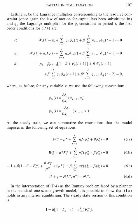
Letting +t be the Lagrange multiplier corresponding to the resource con-straint (once again the law of motion for capital has been substituted in)and 'it the Lagrange multiplier for the ,i constraint in period t, the firstorder conditions for (P.4) are

c: Wc(t)&+t+ :I

i=1

'it ,ic(t)+; :I

i=1

'it+1,ic�(t+1)=0

n: Wn(t)++tFn(t)+ :I

i=1

'it,in(t)+; :I

i=1

'it+1,in�(t+1)=0

k$: &+t+;+t+1[1&$+Fk(t+1)]+;Wk (t+1)

+; :I

i=1

'it ,ik (t+1)+;2 :I

i=1

'it+1,ik�(t+2)=0,

where, as before, for any variable xt we use the following convention:

,ix (t)=�,i

�xt(xt&1 , xt)

,ix�(t)=

�,i

�xt&1

(xt&1 , xt).

At the steady state, we can summarize the restrictions that the modelimposes in the following set of equations:

Wc*&+*+ :I

i=1

'i*(,ic*+;,ic�

*)=0 (6.a)

Wn*++*Fn*+ :I

i=1

'i*(,in*+;,in�

* )=0 (6.b)

&1+;(1&$+Fk*)+;Wk*

+*+( +*)&1 ; :

I

i=1

'i*(,*ik+;,*ik�)=0 (6.c)

c*+g=F(k*, n*)&$k*. (6.d)

In the interpretation of (P.4) as the Ramsey problem faced by a plannerin the standard one sector growth model, it is possible to show that (1.a)holds in any interior equilibrium. The steady state version of this conditionis

1=;[1&$k+(1&{k�)Fk*].



Given the definition of W (in this case), it follows that Wk*=0. If thereare no binding ,i constraints (i.e., if the tax bounds are not binding) then(6.c) directly implies {k

�=0.5

Although for the standard case the formulation in (6) is unnecessarilycumbersome it will prove useful in studying deviations from the basic setupthat are both economically interesting and that yield non-zero limiting taxrates on capital income. In terms of this more general setting it follows that{k

�{0 if and only if

;Wk*+; :I

i=1

'i*(,*ik+;,*ik�){0.

In what follows, we will describe two economic settings that result in thisexpression being non-zero. Our examples will highlight the fact that eitherrents or restrictions on tax codes will result in Wk*{0 or 'i*{0. Con-versely, if either the stock of capital does not enter the planner's utilityfunction (i.e., there are no fixed factors), or the shadow cost, from the pointof view of the planner, of all additional constraints is zero (i.e., 'i*=0, forall i) we are back to the traditional result.

(a) Pure Rents: Inelastic Labor Supply

In this example we study a model that differs from the simple one capitalgood version of the setting of section 2 in only one dimension: labor is sup-plied inelastically. (In independent work, Correia [9] also explores theimplications of fixed factors in a system of territorial taxation and con-cludes that the limiting tax on capital is not zero in the optimal system.)The model then resembles the standard one sector growth model studiedby Cass and Koopmans. We assume that there is a bound on the rate atwhich labor income (a ``pure rent'') can be taxed. This bound might arise,for example, due to political or other types of constraints that we do notexplicitly model. In the absence of such a constraint it is possible to showthat the solution to the problem is similar to that obtained whenever lumpsum taxes are available. It is to prevent this uninteresting (from the pointof view of this paper) outcome that we impose an exogenously given boundon taxation of a factor in fixed supply. In this case the wage rate will begiven by wt=Fn(kt , 1). However, the marginal condition that determinesthe marginal rate of substitution between consumption and leisure as a


5 Although this formulation takes * as given, in the true problem * is such that theappropriate version of (2) (the budget constraint) is satisfied. Since our arguments do notdepend on the value of * (only the fact that it is positive), we can study (P.4) to determinethe properties of optimal steady state taxes.


function of the after-tax real wage, equation (1.b), no longer applies. It canbe shown that, the relevant version of (2) is

:�

t=0

;tuc(t)[ct&(1&{nt )Fn(t)]=uc(0)[[Fk(0)(1&{k

0)+1&$] k0+b0]. (7)

Since taxation of labor income generates only income effects it is clearthat the optimal tax rate is {n

t =1. If this is the bound on labor taxes, it canbe shown that the result in section 2 holds��the limiting capital income taxrate is zero. To highlight the consequences of less than full taxation ofprofits��we will make two additional assumptions. First, that there is anupper bound on the tax rate on labor income given by {� n<1. Second, weassume that the present value of labor income evaluated using the prices[ pt] induced by the solution to the unconstrained planner's problem(described in Proposition 2) and the initial revenue from capital taxationfalls short of the value of government expenditure. With these two assump-tions it follows that the government will choose {n

t ={� n. To simplify thepresentation��and since we are interested in asymptotic results this iswithout loss of generality��from now on we set the initial stock of govern-ment debt equal to zero.

For this problem, it follows that the relevant pseudo utility function Wis

W(c, n, k, *)=u(c)+*[uc(c)(c&(1&{� n) Fn(k, 1))]

and Wk=&*uc(c)(1&{� n) Fkn is different from zero if Fkn{0.The first order conditions for this problem in the steady state are then

given by (6) with the 'i*=0, i=1, ..., I, since there are no constraints otherthan feasibility that are binding in the steady state. The relevant conditionsare

Wc*=+*

1=;[Fk*+1&$]+;Wk*

+*.

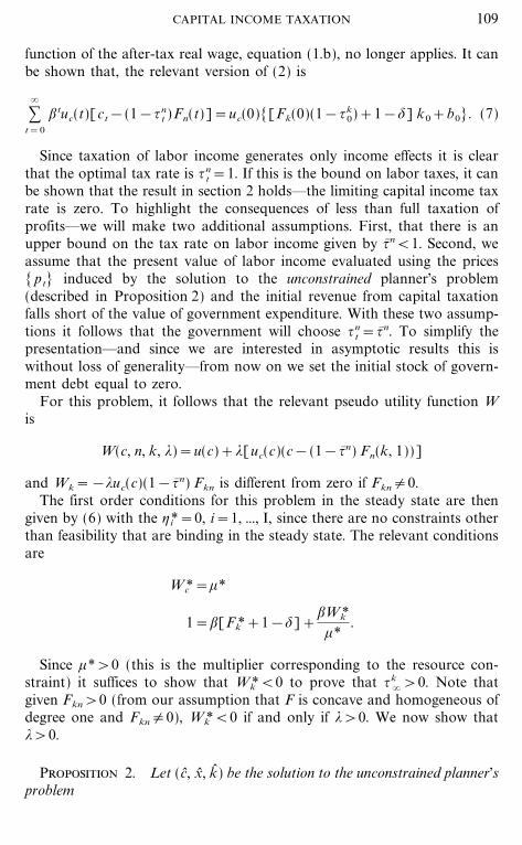
Since +*>0 (this is the multiplier corresponding to the resource con-straint) it suffices to show that Wk*<0 to prove that {k

�>0. Note thatgiven Fkn>0 (from our assumption that F is concave and homogeneous ofdegree one and Fkn{0), Wk*<0 if and only if *>0. We now show that*>0.

Proposition 2. Let (c, x, k� ) be the solution to the unconstrained planner'sproblem



max :�

t=0

;tu(ct)

s.t. ct+kt+1+gt�F(kt , 1)+(1&$)kt

k0>0 givenIf

uc(0) {k0 Fk (k� 0 , 1)k0+ :

�

t=0

;tuc(t) {� nFn(t)< :�

t=0

;tuc(t)gt , (8)

then the solution to the planner's problem is such that *>0.

Before we present the proof of the proposition it is useful to interpret (8).The left hand side is revenue from taxation of capital at time zero plus thepresent value of labor income taxation. Since both k0 and labor are in fixedsupply, taxation of these two factors is equivalent to lump sum taxation.The right hand side is the present value of government spending. Thus, (8)says that, at the prices implied by the first best allocation, revenue fromlump sum taxes falls short of expenditures. This is of course an arbitraryassumption. It is equivalent to ruling out lump sum taxation and withoutit the problem becomes uninteresting as no distortionary taxes are used. Itseems a reasonable assumption in real world applications.

Proof. Consider the following less restrictive version of the Ramseyproblem,

max :�

t=0

;tu(ct)

s.t. ct+gt+kt+1�F(kt , 1)+(1&$)kt

s.t. :�

t=0

;tuc(t)[ct&(1&{� n) Fn(t)]&uc(0)[Fk(0)(1&{k0)+1&$]k0�0,

and let be the Lagrange multiplier associated with the second constraint.Suppose first that *=0. In this case the solution is ``first best'' and givenby (c, k� ).

Note that,

:�

t=0

;tuc(t)(ct&(1&{� n) Fn(t))

= :�

t=0

;tuc(t)[(Fk(t)+1&$)k� t+{� nFn(t)&k� t+1&gt]

=uc(0)(Fk(0)+1&$)k0+ :�

t=0

;tuc(t) {� nFn(t)& :�

t=0

;tuc(t)gt ,



where we used the property that uc(t)=uc(t+1) ;[Fk(t+1)+1&$] fort�0.

Using this equality in the second constraint of the less restrictiveproblem we get

uc(0)(Fk(0)+1&$)k0+ :�

t=0

;tuc(t) {� nFn(t)

& :�

t=0

;tuc(t) gt&uc(0)[(1&{k0) Fk(0)+1&$]k0�0

or

uc(0) {k0 Fk (0)k0+ :

�

t=0

;tuc(t) {� nFn(t)� :�

t=0

;tuc(t) gt .

This contradicts (8) and hence it shows that *>0. K

An alternative, more intuitive argument that shows that *>0 can beconstructed as follows: Denote by V* the maximized value of the planner'sobjective function, and note that the change in V* due to an increase in {k

0

is given by *uc*(0) Fk*(0)k0 . Since increases in {k0 are equivalent to increases

in lump sum taxes and since the higher the level of lump sum taxes thehigher the value of utility, it follows that * must be positive.

Our findings for the case of factor income taxation are reminiscent of theresults of Diamond and Mirrlees [10] and Stiglitz and Dasgupta [25] thatalso show that the existence of pure profits affects the optimal commoditytax schedule.

(b) Two Types of Labor with Equal Taxes

The previous example discussed a particular form of violation of theassumptions that give rise to the Chamley�Judd result: in terms of thepseudo-utility function W of the planner's problem, the term Wk is notzero. Here, we consider the alternative possibility that the constraints ,i arebinding in the steady state. A simple example of such a case is when theplanner cannot distinguish between income from two types of labor.Because of this, we will require that the tax rate on the two types of laborbe equal. This is a convenient way of modeling a more general type of con-straint: restrictions on tax rates. The example we will consider features onehousehold that sells two types of labor to the market, n1 and n2 . This is inthe spirit of Stiglitz [27] where an example is analyzed with two types ofconsumers each with a different type of labor. He analyzes a planner'sproblem with a weighted average of the two consumer's utility functionsand shows that the limiting tax rate on capital income is not zero. Heascribes this finding to redistributional motives that arise due to the



heterogeneity. What we show here is that this finding holds in some caseseven with a representative household that supplies two different types oflabor if the planner is constrained to choose the tax rates on the two typesof labor equally. (An assumption implicit in Stiglitz's work.)

Here, the period utility function of the household is given by u(c, 1&n1 ,1&n2) and the production function is F(k, n1 , n2) .

It can be shown that the W function for this example is given by:

W(c, n1 , n2)=u(c, 1&n1 , 1&n2)+*[uc c&un1n1&un2

n2]

and that the constraints of the planner's problem are

ct+xt+gt�F(kt , n1t , n2t),

kt+1=(1&$)kt+xt ,

,(t)#un1(t) Fn1

(t)&un2(t) Fn2

(t)=0.

The first two constraints describe feasibility while the third uses the firstorder conditions of the household to impose the constraint that the twolabor tax rates should be equal, {n1

={n2for all t. Letting the Lagrange

multipliers on the first and third constraints in the steady state be given by+* and '* respectively, the relevant steady state conditions are

Wc*=+*&'*,c*

W*n1=&+*F*n1

+'*n1

1=;[Fk*+1&$]+;'*,k* �+*.

In section (c), below, we provide a numerical example in which {k�{0.

The equations above indicate when the limiting tax will be zero. If {k�=0,

it must be the case that either '* or ,n* is zero. From the definition of ,,it follows that ,k is given by

,k=un1

Fn1\Fn1k

Fn1

&Fn2k

Fn2+ .

It follows that ,k=0 if and only if

Fn1k

Fn1

=Fn2k

Fn2

.

This condition defines a special class of production functions whichinclude Cobb-Douglas but not the general CES case. To get our



non-zero result we have to assume that our production function is not inthis class.

Alternatively, {k�=0 will hold when '*=0. If the solution has the

property that the restriction that the two tax rates be equal is not bindingthis will be the case. This, however, also requires that the planner'smarginal rate of substitution between consumption and the two types oflabor (as given by the W function) be equal to the household's marginalrate of substitution. In general this will not be the case. The economicreason is that the planner's function includes��in addition to household'sutility function��another term that captures the impact of policy decisionsupon relative prices. Thus, it is only in cases in which this relative priceeffect is irrelevant that the constraint will not be binding and '* will bezero. Examples of this exceptional case include the situation when bothtypes of labor are perfect substitutes in utility and production, since thispins down their relative prices and there is no price effect.

How general is the result that restrictions on tax rates result in non-zerolimiting taxes on capital? There are a variety of other restrictions on taxcodes that can be modeled along similar lines giving the same result. Forexample, in a standard growth model in which factor income from allsources (i.e., both capital and labor) is restricted to be taxed at the samerate, the common limiting rate is non-zero. Alternatively, if pure publicgoods generate private rents which are indistinguishable from payments tocapital, then the limiting tax rate on capital is again non-zero. The com-mon thread in all of these examples is a restriction on the planner's abilityto independently tax income sources. For example, in the case of purerents, this restriction is the assumed inability of the planner to completelytax away these rents.

(c) Tax Calculations for the Two Labor Example

While the examples above show that the tax rate can be non-zero, itremains an open question whether or not the magnitude of this tax rate issignificant. To study this question, we calculate the solution to the optimaltax problem for a specific choice of the example in section (b). In par-ticular, we set

u(c, 1&n1 , 1&n2)=c1&_(1&n1)#1 (1&n2)#2�(1&_)

and

F(k, n1 , n2)=A[bk&\+(1&b)(n1)&\]&��\ (n2)1&�,

where we interpret n1 as skilled labor and n2 as unskilled labor. This utilityfunction can be interpreted as that of a household with two members each



of which is able to supply one unit of leisure to the market each period.Our specification of technology is similar to the nested CES modelestimated by Kwag and McMahon [18]. They consider a setting in whichthe inner function is a CES between skilled labor and physical capital; thisaggregate, in turn, is combined using another CES with unskilled capital.They estimate that the elasticity of substitution between physical capitaland skilled labor is very low (i.e., 0.013), while that between the combinedtotal capital and low skilled labor is in the range of 0.482 to 0.769. Guidedby this we assumed that the elasticity of substitution between n2 and thecomposite between n1 and k is one to simplify the analysis, and we set\=5.0 (which corresponds to an elasticity of 0.16 between capital andskilled labor). This is the rationale behind our interpretation of n1 asskilled labor and n2 as unskilled labor. We chose _=2, �=0.9, #1=&0.2,and #2=&0.8 as a base case and chose g so that the budget would exactlybalance with a flat income tax rate of 200 on all sources of income.

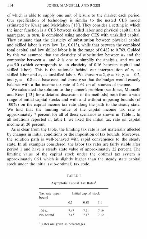
We calculated the solution to the planner's problem (see Jones, Manuelliand Rossi [13] for a detailed discussion of the methods) both from a widerange of initial capital stocks and with and without imposing bounds (of1000) on the capital income tax rate along the path to the steady state.We find that the limiting value of the capital income tax rate isapproximately 7 percent for all of these scenarios as shown in Table 1. Inall solutions reported in table 1, we fixed the initial tax rate on capitalincome at 20 percent.

As is clear from the table, the limiting tax rate is not materially affectedby changes in initial conditions or the imposition of tax bounds. Moreover,the solution path is well-behaved with rapid convergence to the steadystate. In all examples considered, the labor tax rates are fairly stable afterperiod 1 and have a steady state value of approximately 22 percent. Thelimiting value of the capital stock under the optimal tax system isapproximately 0.91 which is slightly higher than the steady state capitalstock under the initial (sub-optimal) tax code.

TABLE I

Asymptotic Capital Tax Rates1

Tax rate upperbound

Initial capital stock

0.5 0.88 1.1

1000 7.47 7.21 7.19No bound 7.47 7.17 7.12

1 Rates are given as percentages.



4. EXTENSIONS AND CONCLUSIONS

Our analysis of optimal factor taxation in dynamic models suggests thatsimple intuitive arguments purporting to explain why the tax rate on capi-tal income is zero in the limit (e.g., due to infinite supply elasticity) are notvery useful. By useful we mean a type of economic intuition that is robustto relative minor changes in the structure of the model. All the differentenvironments discussed in this paper are very close, yet, our conclusionsabout limiting behavior of tax rates are quite different.

A more promising route to understanding the basic forces that drive theasymptotic behavior of optimally chosen tax rates is to delineate featuresof the economy which account for the result. In this paper we showed that,in the context of a model with both human and physical capital, if there areconstant returns to scale in the reproducible factors (no profits), a suf-ficiently rich tax code and no possibilities for relative prices to affect wealththen limiting tax rates on both capital and labor income are zero. Each ofthese three conditions is essential.

Consider the linearity or ``no profits'' condition first. In the model withan inelastic labor supply, the presence of rents result in positive limiting taxrates on capital. Our interpretation is that by distorting the choice ofcapital the planner can ``tax'' the pure rents.

The second element is the richness of the tax code. As the discussion insection 3 (b) shows (as well as the model in section 2 in the absence ofconsumption taxes), the presence of restrictions across tax rates results innon-zero taxes on capital income. More generally, a limited ability to setsufficiently many taxes independently gives the same result. We interpretthis as a standard ``second best'' argument: the imposition of an additionalrestriction (e.g., a restriction across tax rates) calls for a change in how theunaffected policy instruments are chosen. In this case, the restrictions forcea switch from zero to some positive level of capital income taxation in thelong run.

The third element that seems essential is the absence of a role for achange in relative prices as a form of extracting rents from the private sec-tor. In this respect, the model in section 2 in which transfers (a pure rentfrom the point of view of both the consumers and the planner) are notfixed in terms of consumption results in non-zero taxes on labor income.

The reader may wonder if the three features that we have identified over-turn the zero limiting tax result only in the Chamley�Judd environment.Although it is impossible to give an exhaustive answer, we have exploredother environments in which both the Chamley�Judd result obtains andthe violation of one of the three conditions that we identified results innon-zero limiting tax rates. These more general environments allow forheterogeneity (see also Judd [14]), multiple consumption goods and types



of labor and multi-sector settings in which the price of capital in the steadystate is endogenous.

Finally, the model in section 2 suggests that given the linearity assump-tion and a rich tax code, the Ramsey problem has very strong implicationsabout both the timing of tax revenues and the structure of the tax system:Under the optimal scheme, revenue is `front-loaded' and all factors aretreated symmetrically in the limit. This revenue front-loading is a disturb-ing but essential feature of the optimal tax code. Reasonable restrictions onthe time path of deficits (e.g., period by period budget balance) can beshown to undo the zero limiting tax result. In essence, this is another typeof restriction on tax codes not unlike that described in section 3 (b). Thisexample highlights the interdependence of the initial behavior of theoptimal tax code and its limiting properties.

Because of the delicacy of the mapping between the features of theeconomy and the structure of optimal tax codes, further progress willnecessitate a detailed analysis of the entire time path of taxes as in section3 (c). Even for relatively simple examples, this will require a reliance onnumerical methods.

REFERENCES

1. A. B. Atkinson and A. Sandmo, Welfare implications of the taxation of savings, Econom. J.90 (1980), 529�549.

2. A. J. Auerbach, The theory of excess burden and optimal taxation, in ``Handbookof Public Economics, Vol. II'' (A. J. Auerbach and M. Feldstein, Eds.), Elsevier,Amsterdam, 1985.

3. A. J. Auerbach and L. J. Kotlikoff, ``Dynamic Fiscal Policy,'' Cambridge Univ. Press,Cambridge, UK, 1987.

4. R. J. Barro, Government spending in a simple model of endogenous growth, J. Polit.Econom. 98, No. 2 (1990), S103�S125.

5. N. Bull, ``When the Optimal Dynamic Tax is None,'' Working paper, Federal ReserveBoard of Governors, 1992.

6. C. Chamley, Efficient taxation in a stylized model of intertemporal general equilibrium,Internat. Econom. Rev. 26, No. 2 (1985), 451�468.

7. C. Chamley, Optimal taxation of capital income in general equilibrium with infinite lives,Econometrica 54, No. 3 (1986), 607�622.

8. V. V. Chari, L. J. Christiano, and P. J. Kehoe, Optimal fiscal policy in a business cyclemodel, J. Polit. Econom. 102, No. 4 (1994), 617�652.

9. I. Correia, Dynamic capital taxation in small open economies, forthcoming, J. Econom.Dynam. Control, in press.

10. P. A. Diamond and J. Mirrlees, Optimal taxation and public production I: Productionefficiency and II: Tax rules, Amer. Econom. Rev. 61 (1971), 8�27 and 261�278.

11. S. J. Grossman and O. D. Hart, An analysis of the principal agent problem, Econometrica51, No. 1 (1983), 7�45.

12. J. J. Heckman, A life-cycle model of earnings, learning, and consumption, J. Polit.Econom. 84 (1976), S11�S44.



13. L. E. Jones, R. E. Manuelli, and P. E. Rossi, Optimal taxation in models of endogenousgrowth, J. Polit. Econom. 101, No. 3 (1993), 485�517.

14. K. L. Judd, Redistributive taxation in a simple perfect foresight model, J. Public Econom.28 (1985), 59�83.

15. K. L. Judd, The welfare cost of factor taxation in a perfect foresight model, J. Polit.Econom. 95, No. 4 (1987), 675�709.

16. K. L. Judd, `Òptimal Taxation in Dynamic Stochastic Economies,'' Working paper,Stanford University, 1990.

17. R. G. King, `Òbservable Implications of Dynamically Optimal Taxation,'' Working paper,University of Rochester, 1990.

18. Chang Gyu Kwag and Walter W. McMahon, `Èlasticities of Substitution Among Inputs:Comparison of Human Capital and Skilled Labor Models,'' Faculty working paper,University of Illinois Urbana�Champaign, 1992.

19. R. E. Lucas, Jr., On the mechanics of economic development, J. Monet. Econom. 22(1988), 3�42.

20. R. E. Lucas, Jr., Supply side economics: An analytical review, Oxford Econom. Pap. 42(1990), 293�316.

21. R. E. Lucas, Jr. and N. L. Stokey, Optimal fiscal and monetary policy in an economywithout capital, J. Monet. Econom. 12 (1983), 55�93.

22. J. A. Mirrlees, ``The Theory of Moral Hazard and Unobservable Behavior��Part I''Working paper, Nuffield College, Oxford, 1975.

23. J. A. Mirrlees, The theory of optimal taxation, in ``Handbook of MathematicalEconomics'' (K. J. Arrow and M. D. Intrilligator, Eds.), Elsevier, Amsterdam, 1986.

24. F. P. Ramsey, A contribution to the theory of taxation, Econom. J. 37 (1927), 47�61.25. J. Stiglitz and P. S. Dasgupta, Differential taxation, public goods and economic efficiency,

Rev. Econom. Stud. 38 (1971), 151�174.26. J. E. Stiglitz, `Ìnequality and Capital Taxation,'' IMSSS technical report, 1985.27. J. E. Stiglitz, Pareto efficient and optimal taxation and the new welfare economics,

in ``Handbook of Public Economics, Vol. II'' (A. J. Auerbach and M. Feldstein, Eds.),Elsevier, Amsterdam, 1987.

28. C. Yuen, ``Taxation, Human Capital Accumulation and Economic Growth,'' Workingpaper, University of Chicago, 1990.

29. X. Zhu, Optimal fiscal policy in a stochastic growth model, J. Econom. Theory 58 (1992),250�289.


Documents

On the Optimal Taxation of Capital Income - s uhassler-j.iies.su.se/COURSES/DynPubFin/Papers/JonesManuelliRossi... · File: 642J 223801 . By:CV . Date:19:03:97 . Time:10:06 LOP8M