On the Optimization of Heterogeneous MDDs - LSI-CAD · On the Optimization of Heterogeneous MDDs Shinobu Nagayama, Member, IEEE, and Tsutomu Sasao, Fellow, IEEE ... Digital Object

IEEE TRANSACTIONS ON COMPUTER-AIDED DESIGN OF INTEGRATED CIRCUITS AND SYSTEMS, VOL. 24, NO. 11, NOVEMBER 2005 1645

On the Optimization of Heterogeneous MDDsShinobu Nagayama, Member, IEEE, and Tsutomu Sasao, Fellow, IEEE

Abstract—This paper proposes minimization algorithms for thememory size and the average path length (APL) of heterogeneousmultivalued decision diagrams (MDDs). In a heterogeneous MDD,each multivalued variable can take different domains. To rep-resent a binary logic function using a heterogeneous MDD, wepartition the binary variables into groups with different numbersof binary variables and treat the groups as multivalued variables.Since memory size and APL of a heterogeneous MDD dependon the partition of binary variables as well as the ordering ofbinary variables, the memory size and the APL of a heteroge-neous MDD can be minimized by considering both orderings andpartitions of binary variables. The experimental results show thatheterogeneous MDDs can represent logic functions with smallermemory sizes than free binary decision diagrams (FBDDs) andsmaller APLs than reduced ordered BDDs (ROBDDs); the APLsof heterogeneous MDDs can be reduced by half of the ROBDDswithout increasing memory size; and heterogeneous MDDs havesmaller area–time complexities than MDD(k)s.

Index Terms—Area–time complexity, MDD(k), average pathlength (APL), FBDD, heterogeneous MDD, logic simulation,memory size, representation of logic functions, ROBDD.

I. INTRODUCTION

B INARY decision diagrams (BDDs) [5] and multivalueddecision diagrams (MDDs) [16] are extensively used in

logic synthesis [9], logic simulation [1], [13], [19], softwaresynthesis [2], [15], [26], etc. To reduce memory sizes andruntime for these applications, proper optimizations of decisiondiagrams (DDs) are very important. For example, in logicsimulation using DDs [1], [13], [19], minimization of theaverage path length (APL) of DDs reduces the evaluation timeof logic functions, since the evaluation time depends on the pathlength of DDs. In software synthesis using DDs [2], [15], [26],which automatically generates program codes from a functionalspecification, minimization of both memory size and APL ofDDs makes program codes compact and faster, since the codesize and the runtime of the generated program codes depend onthe memory size and path length of DDs. Most optimization al-gorithms for DDs use variable reordering approaches [7]–[11],[14], [20], [21], [23], [28], [32], [38]. However, when MDDsare used to represent binary logic functions, we can use anadditional optimization approach, which is a partition of binaryvariables [12], [29], [33], [36].

Manuscript received July 13, 2004; revised November 15, 2004. This workwas supported in part by the Grant in Aid for Scientific Research of TheJapan Society for the Promotion of Science (JSPS) and the funds from theMinistry of Education, Culture, Sports, Science and Technology (MEXT) viathe Kitakyushu Innovative Cluster Project. This paper was recommended byAssociate Editor I. Stok.

The authors are with the Department of Computer Science and Electronics,Kyushu Institute of Technology, Iizuka 820-8502, Japan (e-mail: [email protected]).

Digital Object Identifier 10.1109/TCAD.2005.852290

To represent a binary logic function using an MDD, wepartition the binary variables into groups and treat each groupas a multivalued variable. In many cases, the groups have thesame number of binary variables [12], [19], [33], [36]. Onthe other hand, in a heterogeneous MDD [29], the groups canhave different numbers of binary variables. Thus, by optimizingboth orderings and partitions of binary variables, we can obtainheterogeneous MDDs that have smaller memory sizes andAPLs than ordinary MDDs with the same group size (calledhomogeneous MDDs). In [36], the optimizations of both order-ings and partitions of binary variables for only homogeneousMDDs are considered.

In this paper, we propose memory size and APL minimiza-tion algorithms for heterogeneous MDDs that consider bothorderings and partitions of binary variables. For BDDs andhomogeneous MDDs, the APL minimization often increasesmemory sizes. On the other hand, for heterogeneous MDDs, theAPLs can be minimized without increasing memory size. Thememory size minimization algorithm for heterogeneous MDDscan reduce both memory sizes and APLs, and the APL mini-mization algorithm for heterogeneous MDDs can reduce APLswithout increasing memory size. By experiments, we show thatboth memory sizes and APLs of heterogeneous MDDs can bereduced to 86% and 67% of reduced ordered BDDs (ROBDDs),respectively, and APLs of heterogeneous MDDs can be reducedby half of the ROBDDs without increasing memory size.

The rest of the paper is organized as follows. Section II showsthe necessary terminology and theorems. Section III proposesmemory size and APL minimization algorithms for heteroge-neous MDDs. And Section IV compares memory sizes andAPLs of heterogeneous MDDs for many benchmark functions.

This paper is an extended version of [30] and [31].

II. PRELIMINARIES

This section defines the necessary terminology and showstheorems. In this paper, we assume that 1) the given logicfunction is completely specified and has no redundant variables;and 2) the reader is familiar with the standard terminology forBDDs and ROBDDs [5].

A. Free BDD

Definition 2.1: An ROBDD has the same variable order onall paths. A free BDD (FBDD) is a BDD that allows differentvariable orders along different paths in the BDD.

An FBDD is a generalization of an ROBDD, so FBDDscan be more compact than ROBDDs by considering differentvariable orders along each path [10], [11], [38].

0278-0070/$20.00 © 2005 IEEE

1646 IEEE TRANSACTIONS ON COMPUTER-AIDED DESIGN OF INTEGRATED CIRCUITS AND SYSTEMS, VOL. 24, NO. 11, NOVEMBER 2005

B. MDD

This section provides a brief definition of MDD. Please referto [16] for more details.Definition 2.2: A BDD represents a binary logic function

fb(x1, x2, . . . , xn) : Bn → B, where B = {0, 1}. An MDDrepresents a multivalued (p-valued) function fm(X1,X2, . . . ,Xu) : Pu → P , where P = {0, 1, . . . , p − 1} and p ≥ 3.

Nonterminal nodes in an MDD for the p-valued functionhave p outgoing edges while nonterminal nodes in a BDDhave two outgoing edges. As with a BDD, there are two typesof MDD: reduced ordered MDD (ROMDD) and free MDD(FMDD). This paper considers only ROMDDs.

C. Partitions of Binary Variables

To represent a binary logic function using an ROMDD, wepartition the binary variables into groups and treat each groupas a multivalued variable.Definition 2.3: Let f(X) be a two-valued logic function,

where X = (x1, x2, . . . , xn) is an ordered set of binary vari-ables. Let {X} denote the unordered set of variables in X .Let Xi ⊆ X . If {X} = {X1} ∪ {X2} ∪ · · · ∪ {Xu}, {Xi} �=φ and {Xi} ∩ {Xj} = φ(i �= j), then (X1,X2, . . . , Xu) isa partition of X . Xi is called a super variable. If |Xi| =ki (i = 1, 2, . . . , u) and k1 + k2 + · · · + ku = n, then a two-valued logic function f(X) can be represented by a multi-valued input two-valued output function that is a mappingf(X1,X2, . . . , Xu) : P1 × P2 × P3 × · · · × Pu → B, wherePi = {0, 1, 2, . . . , 2ki − 1} and B = {0, 1}.

Definition 2.4: A fixed-order partition of X = (x1, x2, . . . ,xn) is a partition (X1,X2, . . . , Xu), where

X1 = (x1, x2, . . . , xk1)

X2 = (xk1+1, xk1+2, . . . , xk1+k2)

...

Xu =(xk1+k2+···+ku−1+1, xk1+k2+···+ku−1+2, . . . , xn−1, xn

)

and |Xi| = ki. That is, in the fixed-order partition of X , thevariable order (x1, x2, . . . , xn) is fixed.

When the variable order is not fixed (i.e., the partition isnot fixed-order partition), we call the partition nonfixed-orderpartition. In this paper, a partition means fixed-order partitionunless stated otherwise.Example 2.1: Consider (X1,X2), which is a fixed-order par-

tition of X , where X = (x1, x2, x3, x4, x5), each xi is a binaryvariable, and the variable order (x1, x2, x3, x4, x5) is fixed.When X1 = (x1, x2) and X2 = (x3, x4, x5), we have k1 = 2,k2 = 3, P1 = {0, 1, 2, 3}, and P2 = {0, 1, . . . , 7}. Note thatX1 takes four values and X2 takes eight values. So, a five-variable logic function f(X) can be represented by the mul-tivalued input two-valued output function f(X1,X2) : P1 ×P2 → B.

Similarly, we show all possible nonfixed-order partitions ofX into (X1,X2), where k1 = 2 and k2 = 3. Since the variable

order (x1, x2, x3, x4, x5) is not fixed, all possible nonfixed-order partitions of X can be considered as

X1 = (x1, x2), X2 = (x3, x4, x5)

X1 = (x1, x3), X2 = (x2, x4, x5)

X1 = (x1, x4), X2 = (x2, x3, x5)

X1 = (x1, x5), X2 = (x2, x3, x4)

X1 = (x2, x3), X2 = (x1, x4, x5)

X1 = (x2, x4), X2 = (x1, x3, x5)

X1 = (x2, x5), X2 = (x1, x3, x4)

X1 = (x3, x4), X2 = (x1, x2, x5)

X1 = (x3, x5), X2 = (x1, x2, x4)

X1 = (x4, x5), X2 = (x1, x2, x3).

D. Heterogeneous MDD

Definition 2.5: When X = (x1, x2, . . . , xn) is partitionedinto (X1,X2, . . . , Xu), an ROMDD representing a multivaluedinput two-valued output function f(X1,X2, . . . , Xu) is calleda heterogeneous MDD. Specially, when k = |Xi| = |X2| =· · · = |Xu|, an ROMDD for f(X1,X2, . . . , Xu) is a homoge-neous MDD and denoted by MDD(k). A heterogeneous MDDrepresents a mapping f : P1 × P2 × . . . × Pu → B while anMDD(k) represents a mapping f : Pu → B, where P ={0, 1, . . . , 2k − 1}, Pi = {0, 1, . . . , 2ki − 1}, and B = {0, 1}.An MDD(k) is a special case of heterogeneous MDDs. In aheterogeneous MDD, nonterminal nodes representing a supervariable Xi have 2ki outgoing edges, where ki denotes thenumber of binary variables in Xi. Similarly, in an MDD(k),nonterminal nodes have 2k outgoing edges.

For n-variable functions f , if n < ku (i.e., n is indivisibleby k), additional redundant binary variables are used to con-struct MDD(k)s. The set of binary variables with such variablesis {X ′} = {x1, x2, . . . , xn, xn+1, . . . , xku}, where |X ′| = ku.Note that f is independent of xn+1, xn+2, . . . , xku.

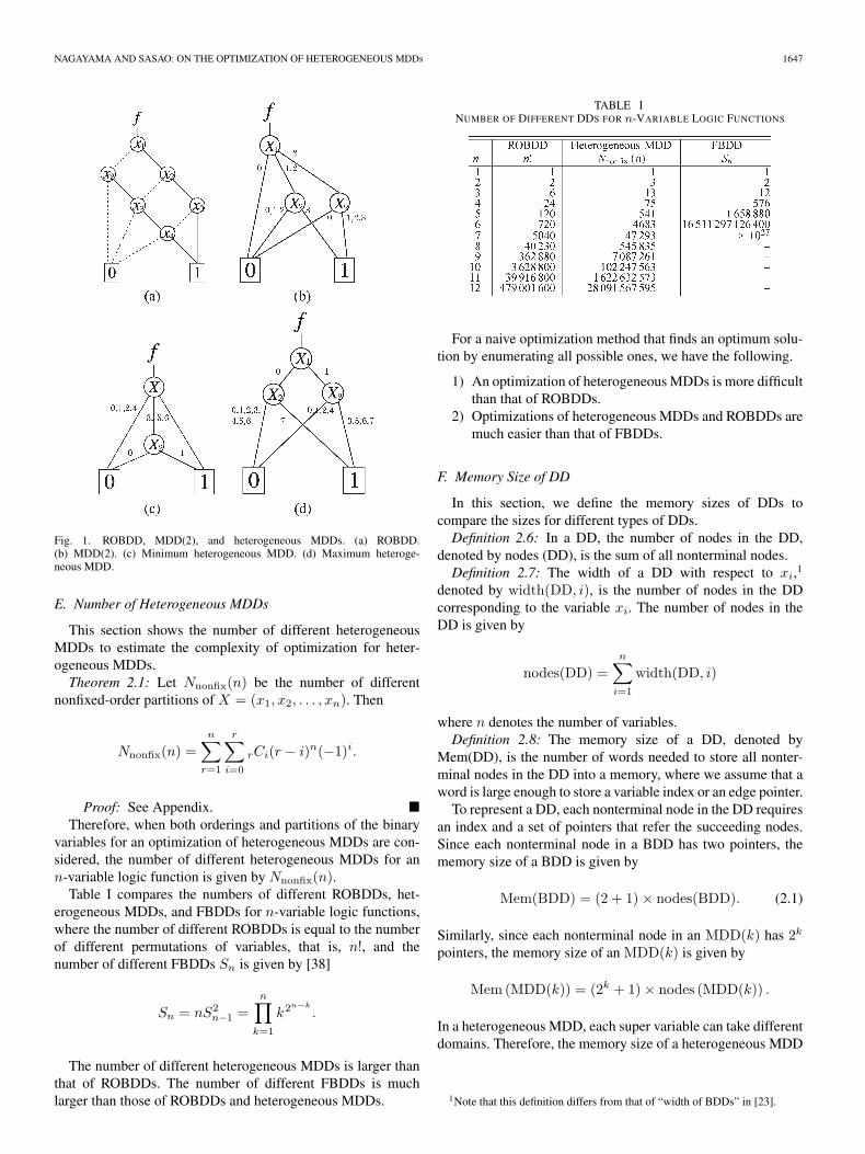
Example 2.2: Consider a logic function f = x1x2x3 ∨x2x3x4 ∨ x3x4x1 ∨ x4x1x2. Fig. 1(a), (b), (c), and (d) repre-sents the ROBDD, MDD(2), and heterogeneous MDDs for f ,respectively. In Fig. 1(a), the solid lines and the dotted lines de-note 1-edges and 0-edges, respectively. In Fig. 1(b), the binaryvariables X = (x1, x2, x3, x4) are partitioned into (X1,X2),where X1 = (x1, x2) and X2 = (x3, x4). In Fig. 1(c), X1 =(x1, x2, x3) and X2 = (x4). This partition produces a heteroge-neous MDD with minimum memory size among heterogeneousMDDs for f . In Fig. 1(d), X1 = (x1) and X2 = (x2, x3, x4).This partition produces a heterogeneous MDD with maximummemory size among heterogeneous MDDs for f .

In this paper, we use shared decision diagrams (SDDs)[22] to represent multiple-output functions F = (f0, f1, . . . ,fm−1) : Bn → Bm, where B = {1, 0}, and n and m denotethe number of input and output variables, respectively. In thefollowing, BDDs and MDDs mean shared BDDs (SBDDs) andshared MDDs (SMDDs), respectively.

NAGAYAMA AND SASAO: ON THE OPTIMIZATION OF HETEROGENEOUS MDDs 1647

Fig. 1. ROBDD, MDD(2), and heterogeneous MDDs. (a) ROBDD.(b) MDD(2). (c) Minimum heterogeneous MDD. (d) Maximum heteroge-neous MDD.

E. Number of Heterogeneous MDDs

This section shows the number of different heterogeneousMDDs to estimate the complexity of optimization for heter-ogeneous MDDs.Theorem 2.1: Let Nnonfix(n) be the number of different

nonfixed-order partitions of X = (x1, x2, . . . , xn). Then

Nnonfix(n) =n∑

r=1

r∑i=0

rCi(r − i)n(−1)i.

Proof: See Appendix. �Therefore, when both orderings and partitions of the binary

variables for an optimization of heterogeneous MDDs are con-sidered, the number of different heterogeneous MDDs for ann-variable logic function is given by Nnonfix(n).

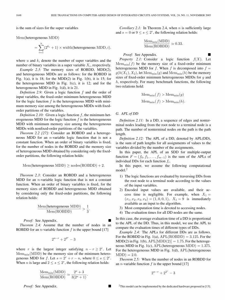
Table I compares the numbers of different ROBDDs, het-erogeneous MDDs, and FBDDs for n-variable logic functions,where the number of different ROBDDs is equal to the numberof different permutations of variables, that is, n!, and thenumber of different FBDDs Sn is given by [38]

Sn = nS2n−1 =

n∏k=1

k2n−k

.

The number of different heterogeneous MDDs is larger thanthat of ROBDDs. The number of different FBDDs is muchlarger than those of ROBDDs and heterogeneous MDDs.

TABLE INUMBER OF DIFFERENT DDS FOR n-VARIABLE LOGIC FUNCTIONS

For a naive optimization method that finds an optimum solu-tion by enumerating all possible ones, we have the following.

1) An optimization of heterogeneous MDDs is more difficultthan that of ROBDDs.

2) Optimizations of heterogeneous MDDs and ROBDDs aremuch easier than that of FBDDs.

F. Memory Size of DD

In this section, we define the memory sizes of DDs tocompare the sizes for different types of DDs.Definition 2.6: In a DD, the number of nodes in the DD,

denoted by nodes (DD), is the sum of all nonterminal nodes.Definition 2.7: The width of a DD with respect to xi,1

denoted by width(DD, i), is the number of nodes in the DDcorresponding to the variable xi. The number of nodes in theDD is given by

nodes(DD) =n∑

i=1

width(DD, i)

where n denotes the number of variables.Definition 2.8: The memory size of a DD, denoted by

Mem(DD), is the number of words needed to store all nonter-minal nodes in the DD into a memory, where we assume that aword is large enough to store a variable index or an edge pointer.

To represent a DD, each nonterminal node in the DD requiresan index and a set of pointers that refer the succeeding nodes.Since each nonterminal node in a BDD has two pointers, thememory size of a BDD is given by

Mem(BDD) = (2 + 1) × nodes(BDD). (2.1)

Similarly, since each nonterminal node in an MDD(k) has 2k

pointers, the memory size of an MDD(k) is given by

Mem(MDD(k)) = (2k + 1) × nodes (MDD(k)) .

In a heterogeneous MDD, each super variable can take differentdomains. Therefore, the memory size of a heterogeneous MDD

1Note that this definition differs from that of “width of BDDs” in [23].


is the sum of sizes for the super variables

Mem(heterogeneous MDD)

=u∑

i=1

(2ki + 1) × width(heterogeneous MDD, i).

where u and ki denote the number of super variables and thenumber of binary variables in a super variable Xi, respectively.

Example 2.3: The memory sizes of ROBDD, MDD(2),and heterogeneous MDDs are as follows: for the ROBDD inFig. 1(a), it is 18; for the MDD(2) in Fig. 1(b), it is 15; forthe heterogeneous MDD in Fig. 1(c), it is 12; and for theheterogeneous MDD in Fig. 1(d), it is 21.Definition 2.9: Given a logic function f and the order of

input variables, the fixed-order minimum heterogeneous MDDfor the logic function f is the heterogeneous MDD with mini-mum memory size among the heterogeneous MDDs with fixed-order partitions of the variables.Definition 2.10: Given a logic function f , the minimum het-

erogeneous MDD for the logic function f is the heterogeneousMDD with minimum memory size among the heterogeneousMDDs with nonfixed-order partitions of the variables.Theorem 2.2 [27]: Consider an ROBDD and a heteroge-

neous MDD for an n-variable logic function that is not aconstant function. When an order of binary variables is fixed,for the number of nodes in the ROBDD and the memory sizeof heterogeneous MDD obtained by considering only the fixed-order partitions, the following relation holds:

Mem(heterogeneous MDD) ≥ nodes(ROBDD) + 2.

Theorem 2.3: Consider an ROBDD and a heterogeneousMDD for an n-variable logic function that is not a constantfunction. When an order of binary variables is fixed, for thememory sizes of ROBDD and heterogeneous MDD obtainedby considering only the fixed-order partitions, the followingrelation holds:

Mem(heterogeneous MDD)Mem(ROBDD)

>13.

Proof: See Appendix. �Theorem 2.4: Assume that the number of nodes in an

ROBDD for an n-variable function f is the upper bound [17]

2n−r + 22r − 3

where r is the largest integer satisfying n − r ≥ 2r. LetMemmin(MDD) be the memory size of the minimum hetero-geneous MDD for f . Let s = 2r + r − n, where 0 ≤ s ≤ 2r.When n is large and 2 ≤ s ≤ 2r, the following relation holds:

Memmin(MDD)Mem(ROBDD)

2s + 33(2s + 1)

.

Proof: See Appendix. �

Corollary 2.1: In Theorem 2.4, when n is sufficiently largeand s = 0 or 9 ≤ s ≤ 2r, the following relation holds:


0.33.

Proof: See Appendix. �Property 2.1: Consider a logic function f(X). Let

Memmin(f) be the memory size of a fixed-order minimumheterogeneous MDD for f . When f is decomposed into f =g(h(X1),X2), let Memmin(g) and Memmin(h) be the memorysizes of fixed-order minimum heterogeneous MDDs for g andh, respectively. For many benchmark functions, the followingtwo relations hold:

Memmin( f) > Memmin(g)

Memmin( f) > Memmin(h).

G. APL of DD

Definition 2.11: In a DD, a sequence of edges and nonter-minal nodes leading from the root node to a terminal node is apath. The number of nonterminal nodes on the path is the pathlength.Definition 2.12: The APL of a DD, denoted by APL(DD),

is the sum of path lengths for all assignments of values to thevariables divided by the number of the assignments.

In this paper, the APL of an SDD for multiple-outputfunction F = (f0, f1, . . . , fm−1) is the sum of the APLs ofindividual DDs for each function fi.

In this paper, we assume the following computationalmodel.2

1) The logic functions are evaluated by traversing DDs fromthe root node to a terminal node according to the valuesof the input variables.

2) Encoded input values are available, and their ac-cess time is negligible. For example, when X1 =(x1, x2, x3, x4) = (1, 0, 0, 1), X1 = 9 is immediatelyavailable as an input to the algorithm.

3) Most computation time is devoted to accessing nodes.4) The evaluation times for all DD nodes are the same.

In this case, the average evaluation time of a DD is proportionalto the APL of the DD. Thus, in this model, we use the APL tocompare the evaluation times of different types of DDs.Example 2.4: The APLs for different DDs are as follows.

For the ROBDD in Fig. 1(a), APL(ROBDD) = 3.125. For theMDD(2) in Fig. 1(b), APL[MDD(2)] = 1.75. For the heteroge-neous MDD in Fig. 1(c), APL(heterogeneous MDD) = 1.375.For the heterogeneous MDD in Fig. 1(d), APL(heterogeneousMDD) = 2.0.Theorem 2.5: When the number of nodes in an ROBDD for

an n-variable function f is the upper bound [17]

2n−r + 22r − 3

2This model can be implemented by the dedicated hardware proposed in [13].


Fig. 2. Exact memory size minimization algorithm for heterogeneous MDDs.

where r is the largest integer satisfying n − r ≥ 2r, there existsa heterogeneous MDD for f that satisfies

APL(heterogeneous MDD) ≤ 2.0

Mem(heterogeneous MDD) ≤Mem(ROBDD).

Proof: See Appendix. �

III. OPTIMIZATION ALGORITHMS OF

HETEROGENEOUS MDDS

Since memory size and APL of a heterogeneous MDD de-pend on the partition of binary variables as well as the orderingof binary variables, the memory size and APL of a heteroge-neous MDD can be minimized by considering both orderingsand partitions of binary variables.

In this section, we formulate the memory size and APL min-imization problems of heterogeneous MDDs considering bothorderings and partitions of binary variables. We also presentexact minimization algorithms to solve them and heuristicminimization algorithms.

A. Memory Size Minimization

We formulate the memory size minimization problem ofheterogeneous MDDs considering both orderings and partitionsof binary variables as follows.Problem 3.1: Given a logic function f(X), find an ordering

and a partition of X that produce the minimum heterogeneousMDD for f .

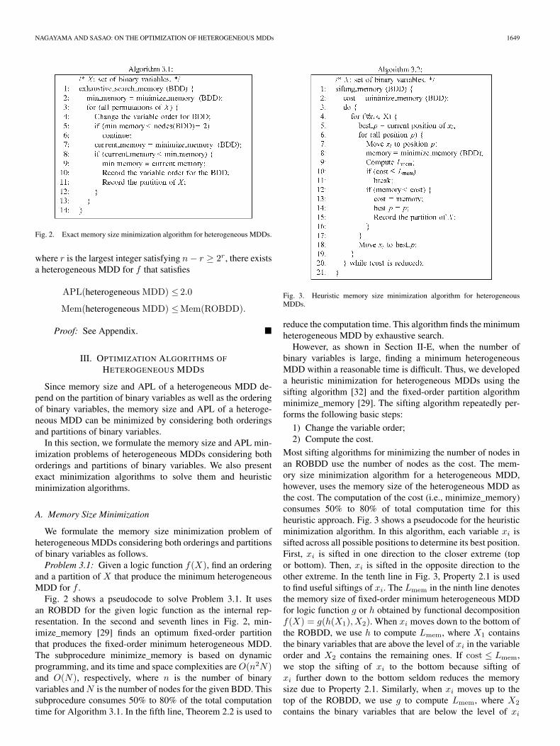
Fig. 2 shows a pseudocode to solve Problem 3.1. It usesan ROBDD for the given logic function as the internal rep-resentation. In the second and seventh lines in Fig. 2, min-imize_memory [29] finds an optimum fixed-order partitionthat produces the fixed-order minimum heterogeneous MDD.The subprocedure minimize_memory is based on dynamicprogramming, and its time and space complexities are O(n2N)and O(N), respectively, where n is the number of binaryvariables and N is the number of nodes for the given BDD. Thissubprocedure consumes 50% to 80% of the total computationtime for Algorithm 3.1. In the fifth line, Theorem 2.2 is used to

Fig. 3. Heuristic memory size minimization algorithm for heterogeneousMDDs.

reduce the computation time. This algorithm finds the minimumheterogeneous MDD by exhaustive search.

However, as shown in Section II-E, when the number ofbinary variables is large, finding a minimum heterogeneousMDD within a reasonable time is difficult. Thus, we developeda heuristic minimization for heterogeneous MDDs using thesifting algorithm [32] and the fixed-order partition algorithmminimize_memory [29]. The sifting algorithm repeatedly per-forms the following basic steps:

1) Change the variable order;2) Compute the cost.

Most sifting algorithms for minimizing the number of nodes inan ROBDD use the number of nodes as the cost. The mem-ory size minimization algorithm for a heterogeneous MDD,however, uses the memory size of the heterogeneous MDD asthe cost. The computation of the cost (i.e., minimize_memory)consumes 50% to 80% of total computation time for thisheuristic approach. Fig. 3 shows a pseudocode for the heuristicminimization algorithm. In this algorithm, each variable xi issifted across all possible positions to determine its best position.First, xi is sifted in one direction to the closer extreme (topor bottom). Then, xi is sifted in the opposite direction to theother extreme. In the tenth line in Fig. 3, Property 2.1 is usedto find useful siftings of xi. The Lmem in the ninth line denotesthe memory size of fixed-order minimum heterogeneous MDDfor logic function g or h obtained by functional decompositionf(X) = g(h(X1),X2). When xi moves down to the bottom ofthe ROBDD, we use h to compute Lmem, where X1 containsthe binary variables that are above the level of xi in the variableorder and X2 contains the remaining ones. If cost ≤ Lmem,we stop the sifting of xi to the bottom because sifting ofxi further down to the bottom seldom reduces the memorysize due to Property 2.1. Similarly, when xi moves up to thetop of the ROBDD, we use g to compute Lmem, where X2

contains the binary variables that are below the level of xi


Fig. 4. Exact APL minimization algorithm for heterogeneous MDDs.

in the variable order and X1 contains the remaining ones.This bounding method is similar to the one shown in [7]that reduces the computation time of the classical sifting fornode minimization.

B. APL Minimization

For any n-variable logic function f(X), the trivial partitionof X , where X = X1 and |X1| = n, produces a heterogeneousMDD with the smallest APL (i.e., APL = 1.0), independentlyof the variable ordering. However, since the memory size of theheterogeneous MDD for the trivial partition is nearly 2n, sucha heterogeneous MDD is too large in most cases. Therefore,an ordering and a partition of X that minimize the APL withina given memory size limitation are sought. We formulate theAPL minimization problem considering both orderings andpartitions of binary variables as follows.Problem 3.2: Given a logic function f(X) and a memory

size limitation L, find an ordering and a partition of X thatproduce the heterogeneous MDD with the minimum APL andwith memory size equal to or smaller than L.

Fig. 4 shows the pseudocode to solve Problem 3.2. In the sec-ond and tenth lines in Fig. 4, the subprocedure minimize_APL[26], [29] finds an optimum fixed-order partition that minimizesthe APL of a heterogeneous MDD. Since it is a recursive pro-cedure, the top level for ROBDD (i.e., level = 1) is required asthe initial argument. The subprocedure minimize_APL is basedon a branch-and-bound method, and its time and space com-plexities are O(2n + n2N) and O(N), respectively, where n isthe number of binary variables and N is the number of nodesfor the given BDD. Although the worst case time complexityfor this subprocedure is high, the actual computation time isshort. For example, when n = 256 (for des), the computationtime for this subprocedure is 0.44 CPU seconds (refer to [29]for more details). This subprocedure consumes 60% to 70%of the total computation time for Algorithm 3.3. Algorithm3.3 finds an optimum solution for Problem 3.2 by exhaustivesearch.

Fig. 5. Heuristic APL minimization algorithm for heterogeneous MDDs.

As well as the memory size minimization, Algorithm 3.3is time consuming for functions with many inputs. Thus,we developed a heuristic APL minimization algorithm forheterogeneous MDDs using a sifting algorithm [32] andthe fixed-order partition algorithm minimize_APL [26], [29].The subprocedure minimize_APL consumes 70%–80% of thetotal computation time for this heuristic approach. Fig. 5 showsa pseudocode for the heuristic APL minimization algorithm. Inthis algorithm, the APL of a heterogeneous MDD is used asthe cost for the sifting algorithm. The APL of a heterogeneousMDD can be computed using a method similar to the APL ofROBDDs in [28]. In the tenth line in Fig. 5, Property 2.1 isused to find useful siftings of xi. If L ≤ Lmem, we stop thesifting of xi because the further sifting of xi seldom finds asmaller memory size than Lmem due to Property 2.1. That is,in most cases, the further sifting of xi produces heterogeneousMDDs with larger memory size than the memory size limitationL when L ≤ Lmem.

IV. EXPERIMENTAL RESULTS

To show the compactness of heterogeneous MDD and theefficiency of optimization algorithms, we compared heteroge-neous MDDs with the different types of DDs using benchmarkfunctions. Experiments were conducted in the following envi-ronment:

• CPU: Pentium 4 Xeon 2.8 GHz;• L1 Cache: 32 KB;• L2 Cache: 512 KB;• Main Memory: 4 GB;• Operating System: redhat (Linux 7.3);• C-Compiler: gcc -O2.


TABLE IIMEMORY SIZES OF ROBDDS, FBDDS, AND HETEROGENEOUS MDDS FOR ALL FOUR-VARIABLE LOGIC FUNCTIONS

A. Comparison With FBDDs

In this section, we compare heterogeneous MDDs withFBDDs to show the compactness of heterogeneous MDDs.

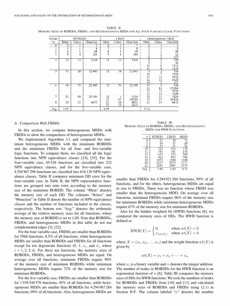
We implemented Algorithm 3.1 and compared the min-imum heterogeneous MDDs with the minimum ROBDDsand the minimum FBDDs for all four- and five-variablelogic functions. To compare them, we classified all the logicfunctions into NPN equivalence classes [24], [35]. For thefour-variable case, 65 536 functions are classified into 222NPN equivalence classes, and for the five-variable case,4 294 967 296 functions are classified into 616 126 NPN equiv-alence classes. Table II compares minimum DD sizes for thefour-variable case. In Table II, the NPN representative func-tions are grouped into nine rows according to the memorysize of the minimum ROBDD. The column “Mem” denotesthe memory size of each DD. The columns “#class” and“#function” in Table II denote the number of NPN equivalenceclasses and the number of functions included in the classes,respectively. The bottom row “Avg.” denotes the arithmeticaverage of the relative memory sizes for all functions, wherethe memory size of ROBDD is set to 1.00. Note that ROBDDs,FBDDs, and heterogeneous MDDs in this table do not usecomplemented edges [3], [22].

For the four-variable case, FBDDs are smaller than ROBDDsfor 5568 functions, 8.5% of all functions, while heterogeneousMDDs are smaller than ROBDDs and FBDDs for all functionsexcept for ten degenerate functions (0, 1, xi, and x̄i, wherei = 1, 2, 3, 4). For these ten functions, the memory sizes ofROBDDs, FBDDs, and heterogeneous MDDs are equal. Onaverage over all functions, minimum FBDDs require 99%of the memory size of minimum ROBDDs while minimumheterogeneous MDDs require 72% of the memory size forminimum ROBDDs.

For the five-variable case, FBDDs are smaller than ROBDDsfor 1 938 548 576 functions, 45% of all functions, while heter-ogeneous MDDs are smaller than ROBDDs for 4 294 967 284functions, 99% of all functions. Also, heterogeneous MDDs are

TABLE IIIMEMORY SIZES OF ROBDDS, FBDDS, AND HETEROGENEOUS

MDDS FOR HWB FUNCTIONS

smaller than FBDDs for 4 294 921 204 functions, 99% of allfunctions, and for the others, heterogeneous MDDs are equalin size to FBDDs. There was no function whose FBDD wassmaller than the heterogeneous MDD. On average over allfunctions, minimum FBDDs require 96% of the memory sizefor minimum ROBDDs while minimum heterogeneous MDDsrequire 67% of the memory size for minimum ROBDDs.

Also for the hidden weighted bit (HWB) functions [6], wecompared the memory sizes of DDs. The HWB function isdefined as

HWB(X) ={

0, when wt(X) = 0xwt(X), when wt(X) > 0

where X = (x1, x2, . . . , xn) and the weight function wt(X) isgiven by

wt(X) = x1 + x2 + · · · + xn

where xi is a binary variable and + denotes the integer addition.The number of nodes in ROBDDs for the HWB function is anexponential function of n [6]. Table III compares the memorysizes of DDs for HWB functions. We took the numbers of nodesfor ROBDDs and FBDDs from [10] and [11] and calculatedthe memory sizes of ROBDDs and FBDDs using (2.1) inSection II-F. The column labeled “n” denotes the number


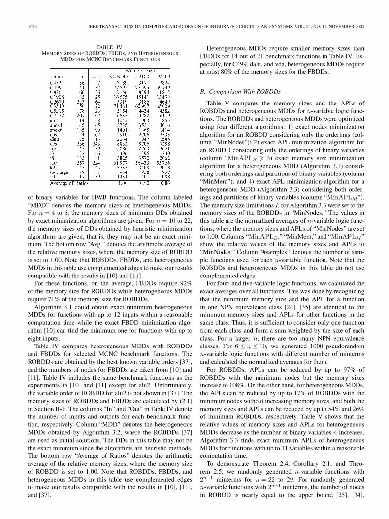
TABLE IVMEMORY SIZES OF ROBDDS, FBDDS, AND HETEROGENEOUS

MDDS FOR MCNC BENCHMARK FUNCTIONS

of binary variables for HWB functions. The column labeled“MDD” denotes the memory sizes of heterogeneous MDDs.For n = 4 to 6, the memory sizes of minimum DDs obtainedby exact minimization algorithms are given. For n = 10 to 22,the memory sizes of DDs obtained by heuristic minimizationalgorithms are given, that is, they may not be an exact mini-mum. The bottom row “Avg.” denotes the arithmetic average ofthe relative memory sizes, where the memory size of ROBDDis set to 1.00. Note that ROBDDs, FBDDs, and heterogeneousMDDs in this table use complemented edges to make our resultscompatible with the results in [10] and [11].

For these functions, on the average, FBDDs require 92%of the memory size for ROBDDs while heterogeneous MDDsrequire 71% of the memory size for ROBDDs.

Algorithm 3.1 could obtain exact minimum heterogeneousMDDs for functions with up to 12 inputs within a reasonablecomputation time while the exact FBDD minimization algo-rithm [10] can find the minimum one for functions with up toeight inputs.

Table IV compares heterogeneous MDDs with ROBDDsand FBDDs for selected MCNC benchmark functions. TheROBDDs are obtained by the best known variable orders [37],and the numbers of nodes for FBDDs are taken from [10] and[11]. Table IV includes the same benchmark functions as theexperiments in [10] and [11] except for alu2. Unfortunately,the variable order of ROBDD for alu2 is not shown in [37]. Thememory sizes of ROBDDs and FBDDs are calculated by (2.1)in Section II-F. The columns “In” and “Out” in Table IV denotethe number of inputs and outputs for each benchmark func-tion, respectively. Column “MDD” denotes the heterogeneousMDDs obtained by Algorithm 3.2, where the ROBDDs [37]are used as initial solutions. The DDs in this table may not bethe exact minimum since the algorithms are heuristic methods.The bottom row “Average of Ratios” denotes the arithmeticaverage of the relative memory sizes, where the memory sizeof ROBDD is set to 1.00. Note that ROBDDs, FBDDs, andheterogeneous MDDs in this table use complemented edgesto make our results compatible with the results in [10], [11],and [37].

Heterogeneous MDDs require smaller memory sizes thanFBDDs for 14 out of 21 benchmark functions in Table IV. Es-pecially, for C499, dalu, and vda, heterogeneous MDDs requireat most 80% of the memory sizes for the FBDDs.

B. Comparison With ROBDDs

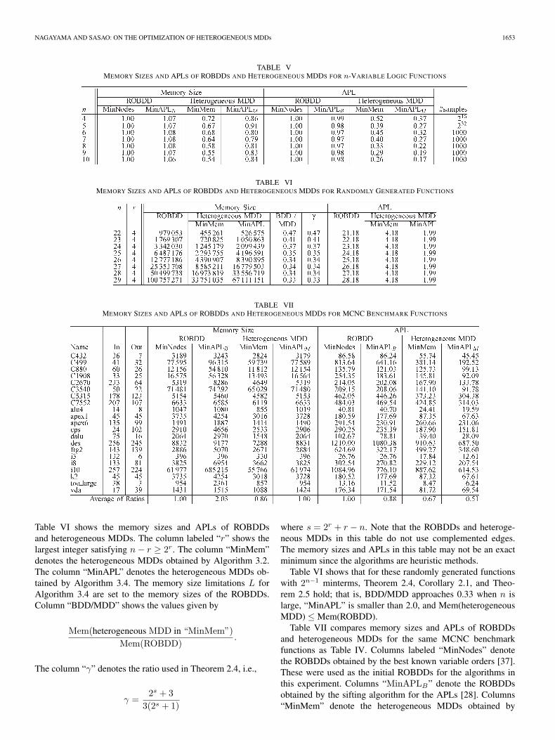
Table V compares the memory sizes and the APLs ofROBDDs and heterogeneous MDDs for n-variable logic func-tions. The ROBDDs and heterogeneous MDDs were optimizedusing four different algorithms: 1) exact nodes minimizationalgorithm for an ROBDD considering only the orderings (col-umn “MinNodes”); 2) exact APL minimization algorithm foran ROBDD considering only the orderings of binary variables(column “MinAPLB”); 3) exact memory size minimizationalgorithm for a heterogeneous MDD (Algorithm 3.1) consid-ering both orderings and partitions of binary variables (column“MinMem”); and 4) exact APL minimization algorithm for aheterogeneous MDD (Algorithm 3.3) considering both order-ings and partitions of binary variables (column “MinAPLM ”).The memory size limitations L for Algorithm 3.3 were set to thememory sizes of the ROBDDs in “MinNodes.” The values inthis table are the normalized averages of n-variable logic func-tions, where the memory sizes and APLs of “MinNodes” are setto 1.00. Columns “MinAPLB ,” “MinMem,” and “MinAPLM ”show the relative values of the memory sizes and APLs to“MinNodes.” Column “#samples” denotes the number of sam-ple functions used for each n-variable function. Note that theROBDDs and heterogeneous MDDs in this table do not usecomplemented edges.

For four- and five-variable logic functions, we calculated theexact averages over all functions. This was done by recognizingthat the minimum memory size and the APL for a functionin one NPN equivalence class [24], [35] are identical to theminimum memory sizes and APLs for other functions in thesame class. Thus, it is sufficient to consider only one functionfrom each class and form a sum weighted by the size of eachclass. For a larger n, there are too many NPN equivalenceclasses. For 6 ≤ n ≤ 10, we generated 1000 pseudorandomn-variable logic functions with different number of mintermsand calculated the normalized averages for them.

For ROBDDs, APLs can be reduced by up to 97% ofROBDDs with the minimum nodes but the memory sizesincrease to 108%. On the other hand, for heterogeneous MDDs,the APLs can be reduced by up to 17% of ROBDDs with theminimum nodes without increasing memory sizes, and both thememory sizes and APLs can be reduced by up to 54% and 26%of minimum ROBDDs, respectively. Table V shows that therelative values of memory sizes and APLs for heterogeneousMDDs decrease as the number of binary variables n increases.Algorithm 3.3 finds exact minimum APLs of heterogeneousMDDs for functions with up to 11 variables within a reasonablecomputation time.

To demonstrate Theorem 2.4, Corollary 2.1, and Theo-rem 2.5, we randomly generated n-variable functions with2n−1 minterms for n = 22 to 29. For randomly generatedn-variable functions with 2n−1 minterms, the number of nodesin ROBDD is nearly equal to the upper bound [25], [34].


TABLE VMEMORY SIZES AND APLS OF ROBDDS AND HETEROGENEOUS MDDS FOR n-VARIABLE LOGIC FUNCTIONS

TABLE VIMEMORY SIZES AND APLS OF ROBDDS AND HETEROGENEOUS MDDS FOR RANDOMLY GENERATED FUNCTIONS

TABLE VIIMEMORY SIZES AND APLS OF ROBDDS AND HETEROGENEOUS MDDS FOR MCNC BENCHMARK FUNCTIONS

Table VI shows the memory sizes and APLs of ROBDDsand heterogeneous MDDs. The column labeled “r” shows thelargest integer satisfying n − r ≥ 2r. The column “MinMem”denotes the heterogeneous MDDs obtained by Algorithm 3.2.The column “MinAPL” denotes the heterogeneous MDDs ob-tained by Algorithm 3.4. The memory size limitations L forAlgorithm 3.4 are set to the memory sizes of the ROBDDs.Column “BDD/MDD” shows the values given by

Mem(heterogeneous MDD in “MinMem”)Mem(ROBDD)

.

The column “γ” denotes the ratio used in Theorem 2.4, i.e.,

γ =2s + 3

3(2s + 1)

where s = 2r + r − n. Note that the ROBDDs and heteroge-neous MDDs in this table do not use complemented edges.The memory sizes and APLs in this table may not be an exactminimum since the algorithms are heuristic methods.

Table VI shows that for these randomly generated functionswith 2n−1 minterms, Theorem 2.4, Corollary 2.1, and Theo-rem 2.5 hold; that is, BDD/MDD approaches 0.33 when n islarge, “MinAPL” is smaller than 2.0, and Mem(heterogeneousMDD) ≤ Mem(ROBDD).

Table VII compares memory sizes and APLs of ROBDDsand heterogeneous MDDs for the same MCNC benchmarkfunctions as Table IV. Columns labeled “MinNodes” denotethe ROBDDs obtained by the best known variable orders [37].These were used as the initial ROBDDs for the algorithms inthis experiment. Columns “MinAPLB” denote the ROBDDsobtained by the sifting algorithm for the APLs [28]. Columns“MinMem” denote the heterogeneous MDDs obtained by


TABLE VIIICPU TIMES (SECOND) FOR MEMORY SIZE

AND APL MINIMIZATION ALGORITHMS

Algorithm 3.2. And columns “MinAPLM ” denote the hetero-geneous MDDs obtained by Algorithm 3.4. The memory sizelimitations L for Algorithm 3.4 were set to the memory sizes ofthe ROBDD in “MinNodes.” In the sifting algorithm [28] andAlgorithm 3.4, the number of rounds of sifting was set to two.Note that the ROBDDs and heterogeneous MDDs in this tableuse complemented edges. The memory sizes and APLs in thistable may not be an exact minimum since the algorithms areheuristic methods. The row labeled “Average of Ratios” repre-sents the normalized averages of memory size and APL, wherethe memory size and the APL of “MinNodes” are set to 1.00.

The sifting algorithm [28] reduced APLs to 88% of“MinNodes,” on average, but doubled the memory sizes. Espe-cially, for C880, C1908, i10, and too_large, the sifting algo-rithm increased the memory sizes significantly. On the otherhand, by considering both orderings and partitions of binaryvariables, Algorithm 3.2 reduced both memory sizes and APLsto 86% and 67% of “MinNodes,” respectively. Algorithm 3.4reduced APLs to 51% of “MinNodes” without increasing thememory size.

C. Comparison of Computation Time for Algorithms

Table VIII compares the computation times for the siftingalgorithm for the APLs [28], Algorithm 3.2, and Algorithm3.4. The values in Table VIII show the CPU times needed toobtain the ROBDDs and heterogeneous MDDs in Table VII, inseconds.

Although Algorithm 3.2 considers both orderings and par-titions of binary variables for memory size minimization, itscomputation time is as short as that of the sifting algorithmthat considers only variable orderings for APL minimization.Algorithm 3.4 requires longer computation times than the othertwo algorithms since Algorithm 3.4 keeps the memory sizewithin the limitation as well as minimizes the APL.

D. Comparison With MDD(k)s

Similarly, we compared heterogeneous MDDs withMDD(k)s.

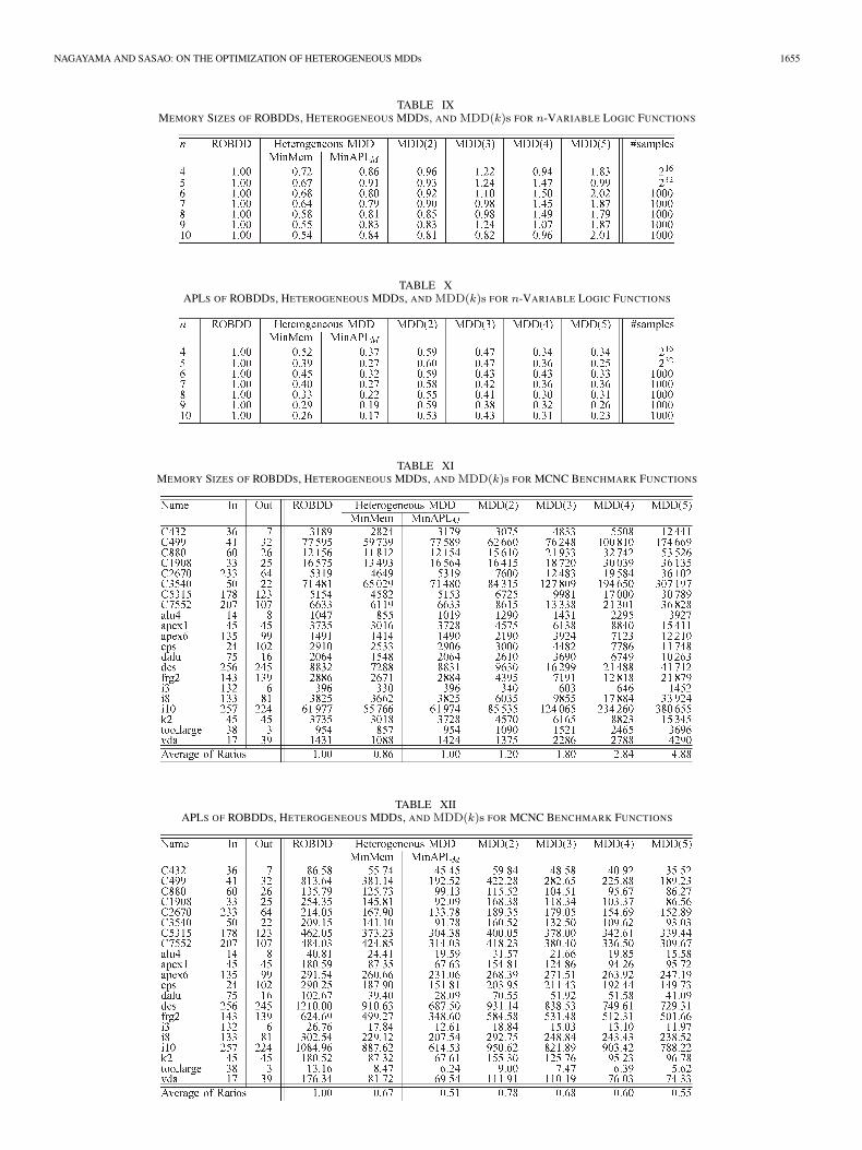
Tables IX and X compare the memory sizes and APLsof ROBDDs, heterogeneous MDDs, and MDD(k)s for n-variable logic functions, respectively. In these tables, MDD(k)shave the exact fewest nodes. The values in these tables arethe normalized averages of n-variable logic functions, wherethe memory sizes and APLs of ROBDD with the fewestnodes (column “ROBDD”) are set to 1.00. Columns “Min-Mem,” “MinAPLM ,” “MDD(2)s,” “MDD(3),” “MDD(4),”and “MDD(5)” show the relative values of the memory sizesand APLs to “ROBDD.”

From Tables IX and X, it can be seen that: for n-variablelogic functions, heterogeneous MDDs obtained by Algorithm3.3 have the APLs as small as MDD(5)s. The memory sizesof MDD(5)s are twice the memory sizes of ROBDDs. On theother hand, heterogeneous MDDs have smaller memory sizesthan ROBDDs.

Tables XI and XII compare the memory sizes and APLs ofROBDDs, heterogeneous MDDs, and MDD(k)s for MCNCbenchmark functions, respectively. MDD(k)s in these ta-bles are obtained by the minimization algorithm in [33].ROBDDs and heterogeneous MDDs are the same as thosein Table VII.

Tables XI and XII show that in heterogeneous MDDs, APLscan be reduced to half of the ROBDDs without increasingmemory sizes. On the other hand, in MDD(k)s, to reducethe APLs to half of the ROBDDs, we need to increase thememory sizes to 488% of the ROBDDs. The APLs of het-erogeneous MDDs obtained by the memory size minimiza-tion algorithm (Algorithm 3.2) are as small as the APLs ofMDD(3)s.

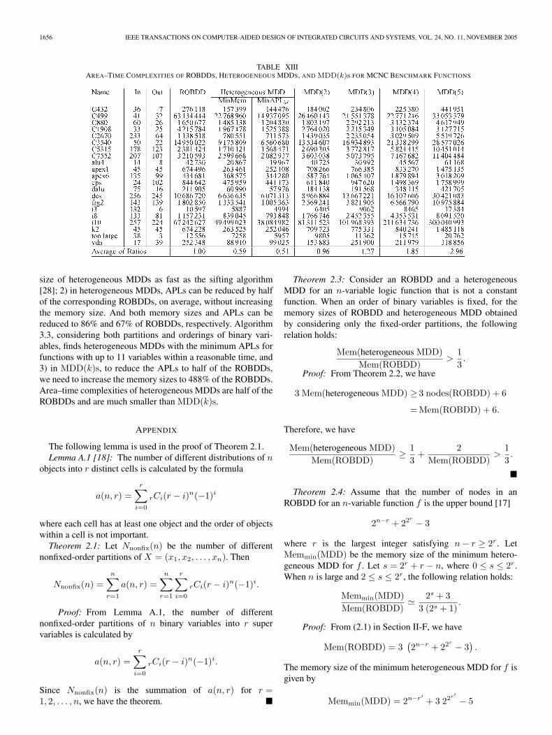
Finally, Table XIII compares the area–time complexities [4],[6], [39] of ROBDDs, heterogeneous MDDs, and MDD(k)sfor MCNC benchmark functions. The area–time complexity isthe measure of computational cost considering both area andtime. It is defined as

AT = area × time.

In this section, the area A corresponds to the memory size andthe time T corresponds to APL.

Table XIII shows that for these benchmark functions,area–time complexities of heterogeneous MDDs are half of theROBDDs and are much smaller than MDD(k)s.

V. CONCLUSION AND COMMENTS

This paper proposed minimization algorithms for the mem-ory size and average path length (APL) of heterogeneous multi-valued decision diagrams (MDDs) that consider both orderingsand partitions of binary variables. The experimental resultsshow that: 1) heterogeneous MDDs represent logic functionsmore compactly than reduced ordered binary decision diagrams(ROBDD s) and free BDDs. Especially, for all five-variablelogic functions, the minimum heterogeneous MDDs require67% of the memory sizes for the minimum ROBDDs, onaverage. Algorithm 3.1 can find exact minimum heterogeneousMDDs for functions with up to 12 inputs in a reasonablecomputation time, and Algorithm 3.2 can reduce the memory


TABLE IXMEMORY SIZES OF ROBDDS, HETEROGENEOUS MDDS, AND MDD(k)s FOR n-VARIABLE LOGIC FUNCTIONS

TABLE XAPLS OF ROBDDS, HETEROGENEOUS MDDS, AND MDD(k)s FOR n-VARIABLE LOGIC FUNCTIONS

TABLE XIMEMORY SIZES OF ROBDDS, HETEROGENEOUS MDDS, AND MDD(k)s FOR MCNC BENCHMARK FUNCTIONS

TABLE XIIAPLS OF ROBDDS, HETEROGENEOUS MDDS, AND MDD(k)s FOR MCNC BENCHMARK FUNCTIONS


TABLE XIIIAREA–TIME COMPLEXITIES OF ROBDDS, HETEROGENEOUS MDDS, AND MDD(k)s FOR MCNC BENCHMARK FUNCTIONS

size of heterogeneous MDDs as fast as the sifting algorithm[28]; 2) in heterogeneous MDDs, APLs can be reduced by halfof the corresponding ROBDDs, on average, without increasingthe memory size. And both memory sizes and APLs can bereduced to 86% and 67% of ROBDDs, respectively. Algorithm3.3, considering both partitions and orderings of binary vari-ables, finds heterogeneous MDDs with the minimum APLs forfunctions with up to 11 variables within a reasonable time, and3) in MDD(k)s, to reduce the APLs to half of the ROBDDs,we need to increase the memory sizes to 488% of the ROBDDs.Area–time complexities of heterogeneous MDDs are half of theROBDDs and are much smaller than MDD(k)s.

APPENDIX

The following lemma is used in the proof of Theorem 2.1.Lemma A.1 [18]: The number of different distributions of n

objects into r distinct cells is calculated by the formula

a(n, r) =r∑

i=0

rCi(r − i)n(−1)i

where each cell has at least one object and the order of objectswithin a cell is not important.Theorem 2.1: Let Nnonfix(n) be the number of different

nonfixed-order partitions of X = (x1, x2, . . . , xn). Then

Nnonfix(n) =n∑

r=1

a(n, r) =n∑

r=1

r∑i=0


Proof: From Lemma A.1, the number of differentnonfixed-order partitions of n binary variables into r supervariables is calculated by

a(n, r) =r∑

i=0


Since Nnonfix(n) is the summation of a(n, r) for r =1, 2, . . . , n, we have the theorem. �

Theorem 2.3: Consider an ROBDD and a heterogeneousMDD for an n-variable logic function that is not a constantfunction. When an order of binary variables is fixed, for thememory sizes of ROBDD and heterogeneous MDD obtainedby considering only the fixed-order partitions, the followingrelation holds:


>13.

Proof: From Theorem 2.2, we have

3 Mem(heterogeneous MDD) ≥ 3 nodes(ROBDD) + 6

= Mem(ROBDD) + 6.

Therefore, we have


≥ 13

+2

Mem(ROBDD)>

13.

�

Theorem 2.4: Assume that the number of nodes in anROBDD for an n-variable function f is the upper bound [17]

2n−r + 22r − 3

where r is the largest integer satisfying n − r ≥ 2r. LetMemmin(MDD) be the memory size of the minimum hetero-geneous MDD for f . Let s = 2r + r − n, where 0 ≤ s ≤ 2r.When n is large and 2 ≤ s ≤ 2r, the following relation holds:


2s + 33 (2s + 1)

.

Proof: From (2.1) in Section II-F, we have

Mem(ROBDD) = 3(2n−r + 22r − 3

).

The memory size of the minimum heterogeneous MDD for f isgiven by

Memmin(MDD) = 2n−r′+ 3 22r′ − 5


where r′ is the largest integer satisfying n − r′ ≥ 2r′+

log2 3 [27].When 2 ≤ s ≤ 2r, the following relation holds:

n − r = 2r + s

2n−r = 2s × 22r

r′ = r.

Then, when n is large, we have

Mem(ROBDD) = 3(2s × 22r

+ 22r − 3)

= 3 (2s + 1)22r − 9

3 (2s + 1)22r

Memmin(MDD) = 2s × 22r

+ 3 × 22r′ − 5

= (2s + 3)22r − 5

(2s + 3)22r

.

Therefore, we have the theorem. �Corollary 2.1: In Theorem 2.4, when n is sufficiently large

and s = 0 or 9 ≤ s ≤ 2r, the following relation holds:


0.33.

Proof:

1) When s = 0 (i.e., n − r = 2r), 2n−r = 22rand r′ = r −

1 hold. Then, we have

Mem(ROBDD) = 3 ×(22r

+ 22r − 3)

= 6 × 22r − 9

Memmin(MDD) = 2n−r′+ 3 × 22r′ − 5

= 2 × 2n−r + 3(22r) 1

2 − 5

= 2 × 22r

+ 3(22r) 1

2 − 5.

Let b = (22r)1/2, then

Mem(ROBDD) = 6b2 − 9 6b2

Memmin(MDD) = 2b2 + 3b − 5 b(2b + 3).

Therefore, when n is large, the following relation holds:


b(2b + 3)6b2

=13

+12b

0.33.

2) From Theorem 2.4, when 9 ≤ s ≤ 2r, the corollaryholds. �

The following lemma is used for proof of Theorem 2.5.Lemma A.2: Let r and r′ be the largest integers satisfying

{n − r ≥ 2r

n − r′ ≥ 2r′+ r′

where n is a nonzero positive integer. Then, for r and r′, thefollowing relation holds:

r − 1 ≤ r′ ≤ r.

Proof: From n − r ≥ 2r, we have

n = 2r + r + a

where a is an integer satisfying 0 ≤ a ≤ 2r.Let r′ = r + b, where b is an integer. Then, from n − r′ ≥

2r′+ r′, we have

n ≥ 2r′+ 2r′ = 2r+b + 2(r + b)

2r + r + a ≥ 2r+b + 2(r + b)

(1 − 2b)2r − r − 2b + a ≥ 0. (A.1)

1) When b > 0, (A.1) does not hold.2) When b = 0, (A.1) holds for r ≤ a ≤ 2r.3) When b < 0, (A.1) holds for 0 ≤ a ≤ 2r.

Since r′ is the largest integer satisfying n − r′ ≥ 2r′+ r′, b

must be the largest integer satisfying (A.1). Therefore, we havethe following relation:

{r′ = r (i.e., b = 0), when r ≤ a ≤ 2r

r′ = r − 1 (i.e., b = −1), when 0 ≤ a ≤ r.

�Theorem 2.5: When the number of nodes in an ROBDD for

an n-variable function f is the upper bound [17]

2n−r + 22r − 3

where r is the largest integer satisfying n − r ≥ 2r, there existsa heterogeneous MDD for f that satisfies


Mem(heterogeneous MDD) ≤Mem(ROBDD).

Proof: When a heterogeneous MDD is represented bytwo super variables: X1 = (x1, x2, . . . , xn−r′) and X2 =(xn−r′+1, xn−r′+2, . . . , xn)


where for simplicity, we assume that the variable order is(x1, x2, . . . , xn). In this case, the memory size of the hetero-geneous MDD is given by

2n−r′+ 1 +

(2r′

+ 1) (

22r′ − 2)

where r′ is the largest integer satisfying n − r′ ≥ 2r′+ r′.

From here, we will prove that this memory size is smaller thanor equal to that of ROBDD

2n−r′+ 1 +

(2r′

+ 1) (

22r′ − 2)≤ 3

(2n−r + 22r − 3

).


By Lemma A.2, we have to only consider two cases: r′ = rand r′ = r − 1.

1) When r′ = r, we have

Mem(ROBDD) = 3(2n−r + 22r − 3

)Mem(heterogeneous MDD)

= 2n−r + 1 + (2r + 1)(22r − 2

)Mem(ROBDD) − Mem(heterogeneous MDD)

= 2(2n−r + 22r

+ 2r)− 22r+r − 8.

From n − r ≥ 2r + r, we have

2(2n−r + 22r

+ 2r)− 22r+r − 8

≥ 2(2n−r + 22r

+ 2r)− 2n−r − 8

= 2n−r + 2(22r

+ 2r)− 8.

Since n ≥ 1 and r ≥ 0, we have

2n−r + 2(22r

+ 2r)− 8 ≥ 0.

2) When r′ = r − 1, we have

Mem(ROBDD) = 3(2n−r′−1 + 22r′+1 − 3

)

Mem(heterogeneous MDD)

= 2n−r′+ 1 +

(2r′

+ 1) (

22r′ − 2)

Mem(ROBDD) − Mem(heterogeneous MDD)

= 2n−r′−1 + 3 × 22r′+1 −(2r′

+ 1)

22r′+ 2r′+1− 8.

From n − r ≥ 2r and r = r′ + 1, we have n − r′ − 1 ≥2r′+1. Then

2n−r′−1 + 3 × 22r′+1 −(2r′

+ 1)

22r′+ 2r′+1 − 8

≥ 22r′+1+ 3 × 22r′+1 −

(2r′

+ 1)

22r′+ 2r′+1 − 8

= 22r′(4 × 22r′ − 2r′ − 1

)+ 2r′+1 − 8.

Since r′ ≥ 0 and (4 × 22r′ − 2r′ − 1) ≥ 6, we have

22r′(4 × 22r′ − 2r′ − 1

)+ 2r′+1 − 8 ≥ 6.

Therefore, the theorem holds. �

REFERENCES

[1] P. Ashar and S. Malik, “Fast functional simulation using branching pro-grams,” in Proc. Int. Conf. Computer-Aided Design (ICCAD), San Jose,CA, Nov. 1995, pp. 408–412.

[2] F. Balarin, M. Chiodo, P. Giusto, H. Hsieh, A. Jurecska, L. Lavagno,A. Sangiovanni-Vincentelli, E. M. Sentovich, and K. Suzuki, “Synthesisof software programs for embedded control applications,” IEEE Trans.Comput.-Aided Des. Integr. Circuits Syst., vol. 18, no. 6, pp. 834–849,Jun. 1999.

[3] K. Brace, R. Rudell, and R. E. Bryant, “Efficient implementation of aBDD package,” in Proc. Design Automation Conf., Orlando, FL, Jun.1990, pp. 40–45.

[4] R. P. Brent and H. T. Kung, “The area–time complexity of binary multi-plication,” J. ACM, vol. 28, no. 3, pp. 521–534, Jul. 1981.

[5] R. E. Bryant, “Graph-based algorithms for Boolean function manipula-tion,” IEEE Trans. Comput., vol. C-35, no. 8, pp. 677–691, Aug. 1986.

[6] ——, “On the complexity of VLSI implementations and graph represen-tations of Boolean functions with application to integer multiplication,”IEEE Trans. Comput., vol. 40, no. 2, pp. 205–213, Feb. 1991.

[7] R. Drechsler, W. Günther, and F. Somenzi, “Using lower bounds duringdynamic BDD minimization,” IEEE Trans. Comput.-Aided Des. Integr.Circuits Syst., vol. 20, no. 1, pp. 51–57, Jan. 2001.

[8] R. Ebendt, W. Günther, and R. Drechsler, “Minimization of the expectedpath length in BDDs based on local changes,” in Proc. Asia and SouthPacific Design Automation Conf. (ASP-DAC), Yokohama, Japan, Jan.2004, pp. 866–871.

[9] M. Fujita, Y. Matsunaga, and T. Kakuda, “On variable ordering ofbinary decision diagrams for the application of multi-level logic synthe-sis,” in Proc. European Design Automation Conf. (EDAC), Amsterdam,The Netherlands, Mar. 1991, pp. 50–54.

[10] W. Günther and R. Drechsler, “Minimization of free BDDs,” in Proc.Asia and South Pacific Design Automation Conf. (ASP-DAC), Wanchai,Hong Kong, Jan. 1999, pp. 323–326.

[11] W. Günther, “Minimization of free BDDs using evolutionary techniques,”in Proc. Int. Workshop Logic Synthesis (IWLS), Loguna Cliffs Marriott,Dana Point, CA, May 2000, pp. 167–172.

[12] H. M. Hasan Babu and T. Sasao, “Heuristics to minimize multiple-valued decision diagrams,” IEICE Trans. Fundam., vol. E83-A, no. 12,pp. 2498–2504, Dec. 2000.

[13] Y. Iguchi, T. Sasao, M. Matsuura, and A. Iseno, “A hardware simulationengine based on decision diagrams,” in Proc. Asia and South PacificDesign Automation Conf. (ASP-DAC), Yokohama, Japan, Jan. 2000,pp. 73–76.

[14] N. Ishiura, H. Sawada, and S. Yajima, “Minimization of binary decisiondiagrams based on exchanges of variables,” in Proc. Int. Conf. Computer-Aided Design (ICCAD), Santa Clara, CA, Nov. 1991, pp. 472–475.

[15] Y. Jiang and B. K. Brayton, “Software synthesis from synchronous speci-fications using logic simulation techniques,” in Proc. Design AutomationConf., New Orleans, LA, Jun. 2002, pp. 319–324.

[16] T. Kam, T. Villa, R. K. Brayton, and A. L. Sangiovanni-Vincentelli,“Multi-valued decision diagrams: Theory and applications,” Int. J.Mult.-Valued Logic, vol. 4, no. 1–2, pp. 9–62, 1998.

[17] H.-T. Liaw and C.-S. Lin, “On the OBDD-representation of generalBoolean function,” IEEE Trans. Comput., vol. 4, no. 6, pp. 661–664,Jun. 1992.

[18] C. L. Liu, Introduction to Combinatorial Mathematics. New York:McGraw-Hill, 1968.

[19] P. C. McGeer, K. L. McMillan, A. Saldanha, A. L. Sangiovanni-Vincentelli, and P. Scaglia, “Fast discrete function evaluation using de-cision diagrams,” in Proc. Int. Conf. Computer-Aided Design (ICCAD),San Jose, CA, Nov. 1995, pp. 402–407.

[20] D. M. Miller and R. Drechsler, “Implementing a multiple-valued deci-sion diagram package,” in Proc. 28th Int. Symp. Multiple-Valued Logic,Fukuoka, Japan, May 1998, pp. 52–57.

[21] ——, “Augmented sifting of multiple-valued decision diagrams,” inProc. 33rd Int. Symp. Multiple-Valued Logic, Tokyo, Japan, May 2003,pp. 375–382.

[22] S. Minato, N. Ishiura, and S. Yajima, “Shared binary decision diagramwith attributed edges for efficient Boolean function manipulation,” inProc. Design Automation Conf., Orlando, FL, Jun. 1990, pp. 52–57.

[23] S. Minato, “Minimum-width method of variable ordering for binary deci-sion diagrams,” IEICE Trans. Fundam., vol. E75-A, no. 3, pp. 392–399,Mar. 1992.

[24] S. Muroga, Logic Design and Switching Theory. New York: Wiley-Interscience, 1979.

[25] S. Nagayama, T. Sasao, Y. Iguchi, and M. Matsuura, “Representationsof logic functions using QRMDDs,” in Proc. 32nd Int. Symp. Multiple-Valued Logic, Boston, MA, May 2002, pp. 261–267.

[26] S. Nagayama and T. Sasao, “Code generation for embedded systemsusing heterogeneous MDDs,” in Proc. 12th Workshop Synthesis and Sys-tem Integration Mixed Information Technologies (SASIMI), Hiroshima,Japan, Apr. 2003, pp. 258–264.

[27] ——, “Compact representations of logic functions using heterogeneousMDDs,” in Proc. 33rd Int. Symp. Multiple-Valued Logic, Tokyo, Japan,May 2003, pp. 247–252.


[28] S. Nagayama, A. Mishchenko, T. Sasao, and J. T. Butler, “Minimiza-tion of average path length in BDDs by variable reordering,” in Proc.Int. Workshop Logic and Synthesis, Laguna Beach, CA, May 2003,pp. 207–213.

[29] S. Nagayama and T. Sasao, “Compact representations of logic functionsusing heterogeneous MDDs,” IEICE Trans. Fundam., vol. E86-A, no. 12,pp. 3168–3175, Dec. 2003.

[30] ——, “Minimization of memory size for heterogeneous MDDs,” inProc. Asia and South Pacific Design Automation Conf. (ASP-DAC),Yokohama, Japan, Jan. 2004, pp. 872–875.

[31] ——, “On the minimization of average path lengths for heteroge-neous MDDs,” in Proc. 34th Int. Symp. Multiple-Valued Logic, Toronto,Canada, May 2004, pp. 216–222.

[32] R. Rudell, “Dynamic variable ordering for ordered binary decision di-agrams,” in Proc. Int. Conf. Computer-Aided Design (ICCAD), SantaClara, CA, Nov. 1993, pp. 42–47.

[33] T. Sasao and J. T. Butler, “A method to represent multiple-output switch-ing functions by using multi-valued decision diagrams,” in Proc. 26thInt. Symp. Multiple-Valued Logic, Santiago de Compostela, Spain,May 1996, pp. 248–254.

[34] T. Sasao, “Ternary decision diagrams survey,” in Proc. 27th Int. Symp.Multiple-Valued Logic, Antigonish, NS, Canada, May 1997, pp. 241–250.

[35] ——, Switching Theory for Logic Synthesis. Norwell, MA: Kluwer,1999.

[36] F. Schmiedle, W. Günther, and R. Drechsler, “Dynamic re-encodingduring MDD minimization,” in Proc. 30th Int. Symp. Multiple-ValuedLogic, Portland, OR, May 2000, pp. 239–244.

[37] F. Somenzi, CUDD: CU Decision Diagram Package Release 2.3.1.Boulder, CO: Univ. Colorado, 2001.

[38] K. Takagi, H. Hatakeda, S. Kimura, and K. Watanabe, “Exact mini-mization of free BDDs and its application to pass-transistor logic opti-mization,” IEICE Trans. Fundam., vol. E82-A, no. 11, pp. 2407–2413,Nov. 1999.

[39] C. D. Thompson, “Area–time complexity for VLSI,” in Proc. Ann. Symp.Theory Computing, Atlanta, GA, May 1979, pp. 81–88.

Shinobu Nagayama (S’02–M’04) received the B.S.and M.E. degrees from the Meiji University, Kana-gawa, Japan, in 2000 and 2002, respectively, and thePh.D. degree in computer science from the KyushuInstitute of Technology, Iizuka, Japan, in 2004.

He is now a Postdoctoral Researcher in KyushuInstitute of Technology. His research interest in-cludes decision diagrams, software synthesis, andembedded systems.

Tsutomu Sasao (S’72–M’77–SM’90–F’94) re-ceived the B.E., M.E., and Ph.D. degrees in electron-ics engineering from the Osaka University, Osaka,Japan, in 1972, 1974, and 1977, respectively.

He has held faculty/research positions at OsakaUniversity, the IBM T.J. Watson Research Center,Yorktown Heights, NY, and the Naval PostgraduateSchool, Monterey, CA. He is currently a Professor atthe Department of Computer Science and Electron-ics, Kyushu Institute of Technology, Iizuka, Japan.His research areas include logic design and switching

theory, representations of logic functions, and multiple-valued logic. He haspublished more than nine books on logic design, including Logic Synthesisand Optimization, Representation of Discrete Functions, Switching Theory forLogic Synthesis, and Logic Synthesis and Verification (Kluwer Academic, 1993,1996, 1999, and 2001) respectively.

Dr. Sasao has served as Program Chairman for the IEEE InternationalSymposium on Multiple-Valued Logic (ISMVL) many times. Also, he was theSymposium Chairman of the 28th ISMVL held in Fukuoka, Japan, in 1998. Hereceived the National Institute of Water and Atmospheric Research (NIWA)Memorial Award in 1979, Distinctive Contribution Awards from the IEEEComputer Society Technical Committee on Multiple-Valued Logic (MVL-TC)in 1987, 1996, and 2004 for papers presented at ISMVLs, and the TakedaTechno-Entrepreneurship Award in 2001. He has served as an Associate Editorof the IEEE TRANSACTIONS ON COMPUTERS.

Documents

On the Optimization of Heterogeneous MDDs - LSI-CAD · On the Optimization of Heterogeneous MDDs Shinobu Nagayama, Member, IEEE, and Tsutomu Sasao, Fellow, IEEE ... Digital Object